Early-Time Stability of Decelerating Shocks
Abstract
We consider the decelerating shock instability of Vishniac for a finite layer of constant density. This serves both to clarify which aspects of the Vishniac instability mechanism depend on compressible effects away from the shock front and also to incorporate additional effects of finite layer thickness. This work has implications for experiments attempting to reproduce the essential physics of astrophysical shocks, in particular their minimum necessary lateral dimensions to contain all the relevant dynamics.
Keywords:
hydrodynamics – instabilities – shock wavesI Introduction
[1] outlined a theory of instabilities for a system of a decelerating shock accreting mass, modeled as a thin mass shell layer possessing no internal structure. In [2], the theory was expanded to include a layer of post-shock material, exponentially attenuating in density. Other work ([3, 4]; among others) has described the perturbation of self-similar solutions for the post-shock flow. The present work complements these investigations, modeling the post-shock flow as a finite thickness layer of constant density and considering both compressible and incompressible post-shock states. This allows us both to more clearly understand which mechanisms depend on the compressibility of the shocked gas and which are common to any shock system undergoing deceleration.
Early in the lifetime of an impulsively driven shock, when the post-shock layer thickness is small compared to its compressible length scale, an exponential scale cannot be formed and the density profile may be closely approximated by a square wave, as a fluid everywhere of constant density. In the shock’s frame, upstream fluid is entering the shock with a speed and exiting it with a speed , where is the inverse compression ratio associated with the shock, including both the viscous density increase and any subsequent, localized further density increase in consequence of radiative cooling [5].
We have also in mind throughout this paper experiments [6, 7, 8] that have been carried out to investigate radiating shock dynamics. Experiments of this type are often designed to be scaled to relevant astrophysical investigation [9]. The particular experiments of [6] feature characteristic shock velocities of over 100 km/sec, shock tubes with 625 m diameters, and strong deceleration throughout the shocks’ lifetimes.
II System of a Decelerating Shock with a Dense Downstream Layer
We consider the shock in its own, decelerating frame. The system is depicted in Figure 1. The shock is placed at , with flow entering it from the negative direction at speed , density , and with negligible thermal pressure. Flow is exiting the shock toward positive with speed , density , and isotropic pressure . We will model the downstream, rear layer as a constant density region of finite, increasing thickness from to . The rear surface of the dense layer will be taken to be a free interface at constant pressure. Beyond the rear layer will be taken as a region of constant thermal pressure .
The native surface wave modes in the system will be right- and left-propagating waves on the two surfaces of the dense layer, leading to four modes in total. As drawn in Figure 1, the upper surface, a material discontinuity, is stable if the shock frame is decelerating and is characterized by surface gravity modes. The bottom surface, a shock at which compressibility is not suppressed, will feature propagating acoustic modes. The waves which appear in our coupled system will be modifications of these waves which appear on these surfaces in isolation. In particular, the modified acoustic waves along the shock surface will be identified as bending modes of the entire dense layer.
In order to understand the fundamental cause of the instability, we will here be considering the fluid both ahead and behind the shock to be held at (different) densities constant in both space and time. This practice is described and defended by [10], who in their book “consider constant-density hypersonic flows, though we should never consider the fluid in a hypersonic flow as incompressible.” The pressure profile behind the shock is hydrostatic, , which leads to increasing pressure at the shock front when the shock is decelerating. Perturbations to density by the waves under investigation will be discussed.
III Linear Perturbations of the System
III.1 Solutions Inside the Post-Shock Fluid
We begin with the inviscid fluid equations
| (1) | |||
| (2) |
with total velocity and . We will insert the perturbation only in the continuity equation; the coupling of to the frame’s acceleration will be suppressed. This allows us to ignore mode purely internal to the layer, concentrating on the overall shock and layer system. Since log log for any reasonable density perturbations, we expect the dynamics of the system to be dominated by the compression at the shock. The omission of the term is also required for consistency with the assumption of our square wave density profile; the system will otherwise begin to evolve into an exponential atmosphere.
We first let the perturbations have time and space dependence as , with real and complex. We then linearize the - and - components of the momentum equation to obtain
| (3) |
| (4) |
We expressed the perturbed continuity equation in terms of perturbed pressure,
| (5) |
where . We solve Equation 3 for using Equation 5, and discard terms of order to obtain
| (6) |
and insert that into Equation 4 to obtain a new equation for z-momentum:
| (7) |
which can now be written as a differential equation for (taking and constant throughout the post-shock layer),
| (8) |
For a treatment of the problem where varies through the layer, see Appendix A.
We define
| (9) |
which describes the effective lateral wavenumber. As a wave approaches the acoustic case, , the wave becomes purely longitudinal and tends toward zero. Equation 8 has the general solution
| (10) |
The system accordingly has three boundary conditions at its two interfaces: the shock and the rear surface. We note that the shock frame’s acceleration does not appear in the general form of the perturbations; it will enter into the system through the boundary conditions.
The last term in Equation 10 is a consequence of the background flow and is closely connected with structures convecting downstream with that velocity. It is instructive to consider the general solution for in the frame of the rear surface. We introduce the coordinate . In addition, we will now write explicitly the implicit time-dependence . The general solution is . We see that the third term has no time-dependence in the frame of the rear layer. In the frame of the rear surface, these flow structures are generated by perturbations in the shock surface as the shock passes some point in space, and do not evolve further. Therefore, in the frame of the shock, this term describes flow structures convecting downstream through the flow with constant velocity . We take the shock to have been perfectly planar at the instant, some time past, at which the shock’s deceleration and rear layer formation began. This allows us to explicitly set at the rear layer. We assume however that the perturbation began sufficiently early in time that our treatment using Fourier modes is sufficient, so no further information from initial conditions will be incorporated at this time.
III.2 Infinitely Thin Layer
We recall that the dispersion relation for the thin shell instability in its most simple form, without the effects of compression, is in [2] written in the form
| (11) |
where is the areal mass density of the (infinitely) thin layer, and all other variables are as we have defined them. Early work [1] derived this expression for a shock of infinitesimal height but finite areal density. Such a shock, maintaining an infinitely thin layer height while continuing to accrete mass from the incoming flow, would in our analysis be described as the limit of an infinite compression, . We should expect solutions we obtain for layers of finite thickness to approach Equation 11 in this limit.
III.3 Free Rear Surface
We construct the boundary condition describing a free layer at by applying at , with . Using Equation 10 and our earlier expression for , Equation 6, the boundary condition becomes
| (12) |
where has been explicitly set to zero as discussed above. Equation 12 is a boundary condition well known to generate surface gravity waves, when and when paired with a rigid boundary condition at .
At the shock surface, we must perturb the shock momentum jump condition in the frame of the moving shock. The perturbed shock surface moving upward in Figure 1 sees a weaker incoming flow. In addition, by raising the shock surface in the hydrostatic pressure field, the effective post-shock pressure drops by an amount . Our jump condition has now become
| (13a) | |||
| from which we obtain a boundary condition (using , , and our earlier expression for in Equation 6) | |||
| (13b) | |||
The expression for comes from conservation of mass across the shock. With density perturbations suppressed, as discussed above, we have a balance of mass flux with entering and leaving the shock, with the shock moving at speed .
| (14a) | |||
| implying (with ) | |||
| (14b) | |||
The third boundary condition comes from oblique shock relations. Letting be the angle of the shock surface perturbation, continuity of the tangential flow requires to first order Applying the continuity equation of Equation 5 just downstream of the shock, and applying Equations 6 and 14b
| (15a) | |||
| which evaluates to | |||
| (15b) | |||
Simultaneously applying these three conditions (equations 12, 13b, and 15b) on , one demands for nonzero solutions that the determinant of the matrix of coefficients of , , and , shown collected in Equation 16, must be zero,
| (16) |
From this one obtains, with some manipulation, the dispersion relation,
| (17) |
We will take, as in [2], the product to be equivalent to an average sound speed squared , which we shall not henceforth distinguish from the sound speed of material compressibility. The qualitative classification of solutions to Equation 17 depends strongly on the layer thickness , specifically on its relation to the compressible scale height . We shall explore this dependence in what follows.
We will now investigate the range in which wavelengths of perturbations are not much shorter than , and will approximate . The existence of the critical is easiest to see in the limit of very strong, highly compressive shocks ( while in such a way that and remain constant). By expanding , we may write the dispersion relation as,
| (18a) | ||||
| where we have introduced scale factors | ||||
| (18b) | ||||
| (18c) | ||||
| (18d) | ||||
For strong shocks, , in which any effects of strong radiation are included in as an effective polytropic index describing the total density increase at the shock [11]. is typically close to 1. Solutions of Equation 18, shown in Figure 2, yield instability for in the range , centered around a wavenumber of maximum instability , where
| (19a) | ||||
| (19b) | ||||
| (19c) | ||||
We find that and are real for , requiring and , conditions defining a decelerating shock and a layer width shorter than a scale height.
For the high compression limit , , the critical wavenumbers take the values
| (20a) | ||||
| (20b) | ||||
| (20c) | ||||
The solutions for growth rate at the fastest growing wavelength are
| (21) |
which allow us to verify that for , remains small, validating our assumption.
In the opposite limit of shock strength, as and the shock is removed from the system, and the bending waves asymptotically approach unmodified acoustic waves at high .
III.4 Limiting Behavior of Solutions
To investigate individually the effect of various terms, we may make several further simplifying assumptions to Equation 17. We will consider both the high compression limit, , as well as the limit of negligible compressibility, . We then obtain from Equation 17 the equation
| (22) |
The term in Equation 22, which stems from the same physical source as the term discarded in Equation 6b of [2], contributes to damping and shock stability in the high limit. It was demonstrated in early work, such as that by [12], that we expect stability for shocks separating two simple spaces of homogenous material. Accordingly, in systems with decelerating shock-bounded dense layers, as we tend to wavelengths short compared to the width of the layer, the dynamics must approach this stable limit [13]. The correct rate of damping is however beyond the scope of our assumptions. [14] have shown that the acoustic modes within the shocked material, which we have suppressed, play a role in stabilizing the shock.
The limit of an indefinitely thin layer is approached, in the notation of Equation 22, by taking the limit of negligible post-shock flow , rearranging the dispersion relation as
| (23) |
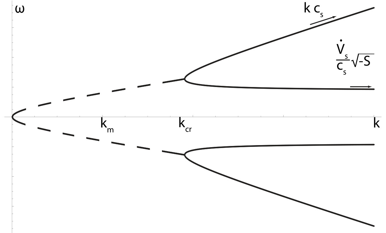
This shows that, in these limits, we regain the form of the Vishniac dispersion relation (Equation 11). We also see that, for less than the scale height and , the quantity in square brackets becomes negative, while this quantity is positive for large or positive . This means that the solutions to Equation 23 have the signature of the Vishniac thin layer dispersion for an accelerating shock, except when lies within a scale height for a decelerating shock, . Solutions when is in that range appear as shown in Figure 3.
The region of instability is , with a maximum growth at , where
| (24a) | ||||
| (24b) | ||||
Compared with Equations 20 and Figure 2, we see that the principal result of removing the effects of compressibility is to eliminate the region of stability near . We also see that the bending modes now travel asymptotically for high with the full speed of sound, where previously they moved at .
IV Post-Shock Flow Patterns
Figure 4 shows a numerical solution of Equation 22 for a shock system with three different thicknesses. The shock system has a scale height of . One can see that for the very thin layer in Fig 4(a), the flow pattern is most similar to that of a surface wave. As the post-shock layer increases in thickness through Figs 4(b) and (c), the flow pattern evolves to contain vorticity features. We speculate that the transition at the scale height corresponds to a layer thickness in which a complete cell is localized.
We remark that in the numerical solution of Equation 22 we find that the shock and rear surfaces’ perturbations achieve different phase. Since the fluid inside the layer is constant in density, this will lead to a corresponding perturbation of areal density of the layer that might be observed. The physical connection is therefore maintained with the theory described by [1], in which dynamics causing variation in areal density of the post-shock layer leads to overstability in the shock. These plots may be compared with Figures 7-10 of [3], which show similar vortical structure, though without boundary phase shifting.
V Further Considerations and Conclusions
V.1 Connections to the Infinitely Thin System
We have seen that the characteristic fourth-order nature of the Vishniac instability, as derived in Equation 17, follows from allowing perturbations on both surfaces of the post-shock layer. We note that while the Vishniac derivations contain an instability source in the product , our dispersion relation in Equation 17 contains a source term . This difference follows from Vishniac’s assumption that the post-shock layer is thin and that the difference between thermal backing pressure and ram pressure together with geometric factors (such as spherical divergence of the shock) are the fundamental sources of the deceleration. We have instead worked with planar shocks and assumed deceleration to stem primarily from mass accumulation and energy loss from the system, for example by strong radiative cooling, and a hydrostatic distribution within the layer to be the dominant contributor to pressure variation.
Despite these differences in approach, we can in fact derive Equation 11 from Equation 23 immediately. We identify the sound speed at the shock surface with local post-shock fluid variables
| (25) |
We have implicity set the polytropic index , which is consistent with our assumption in Equation 23 that we are in the infinitely compressive limit . However, we do not expect Equation 25 to be in general consistent with our other definitions of , except in the limit of an infinitely thin shell, . Keeping this in mind, we see that inserting Equation 25 and into the term in square brackets in Equation 23, one obtains Equation 11. Our derivation therefore is found to agree with the earlier results of Vishniac in the appropriate limits.
We comment on the different solutions to Equations 11, 18, and 23. The oscillating instability which exists when is the case of interest in which collective modulation of the boundary layers results in the growth of structure. The non-oscillating instability which appears when is recognized as the Rayleigh-Taylor instability of the rear layer under acceleration.
The non-oscillating solutions of Equations 18 and 23 when but are of a different nature than the other cases. The system under perturbation was constructed by equating the pressure immediately behind the shock with the ram pressure of the incoming material. The pressure profile then decreased hydrostatically with distance from the shock. When exceeds a scale height, the most distant pressures obtained in this fashion become negative. The “instability” in this case is a response of the system to inconsistent initial conditions. In Vishniac’s equation, this corresponds to the case where one assigns .
Compared to Equation 11, Equations 17 and 23 have the property of being written in terms of the rear layer height and variables defined locally at the compression front, with few assumptions regarding the structure throughout the layer, while Equation 11 is properly understood as dealing with quantities averaged over the layer height. This difference allows one to straightforwardly identify from Equation 23 the combination of system variables which lead to the transition at the scale height. Equation 17 features the same behavior extended to general post-shock and finite , with appropriate corrections leading to transition at a fraction of the scale height. We expect the constant density solution to be applicable within a scale height, beyond which modeling the layer as a region of constant density will not be as appropriate as an exponential or self-similar profile.
V.2 Experimental Observations
We conclude with some discussion of experiments featuring strongly decelerating planar shocks. Experiments which intend to reproduce this instability must feature sufficient lateral space for the growing perturbations. Very early in the experiment’s evolution, the post-shock layer thickness will be necessarily small, and we assume . We see from the results of the proceeding compressible analysis (Equations 20 and 21) that to allow maximum growth one must afford the experiment lateral dimensions , where is a characteristic or average layer thickness of the system. The evolution will occur within a growth time scale . Conversely, if one wishes to eliminate entirely this instability one should construct an experiment with lateral dimensions . For the experiments discussed above by [6], the values of preferred minimum distance and time are approximately 400 - 500 m and 9 - 13 ns, conditions which are achievable by the reported experiment.
References
- [1] E. T. Vishniac, ApJ 274, 152 (1983).
- [2] E. T. Vishniac and D. Ryu, ApJ 337, 917 (1989).
- [3] E. Bertschinger, ApJ 304, 154 (1986).
- [4] D. Kushnir, E. Waxman, and D. Shvarts, ApJ 634, 407 (2005).
- [5] R. P. Drake, High-Energy-Density Physics (Springer, 2006).
- [6] A. B. Reighard, R. P. Drake, K. K. Dannenberg, D. J. Kremer, M. Grosskopf, E. C. Harding, D. R. Leibrandt, S. G. Glendinning, T. S. Perry, B. A. Remington, et al., Phys. Plasmas 13, 082901 (2006).
- [7] S. Bouquet, C. Stéhlé, M. Koenig, J.-P. Chièze, A. Benuzzi-Mounaix, D. Batani, S. Leygnac, X. Fleury, H. Merdji, C. Michaut, et al., Phys. Rev. Lett. 92, 225001 (2004).
- [8] J. C. Bozier, G. Thiell, J. P. Le Breton, S. Azra, M. Decroisette, and D. Schirmann, Phys. Rev. Lett. 57, 1304 (1986).
- [9] B. A. Remington, R. P. Drake, and D. D. Ryutov, Reviews of Modern Physics 78, 755 (2006).
- [10] W. Hayes and R. Probstein, Hypersonic Flow Theory (Academic Press, 1966).
- [11] Edison Liang and Katherine Keilty, ApJ 533, 890 (2000).
- [12] N. C. Freeman, Royal Society of London Proceedings Series A 228, 341 (1955).
- [13] E. T. Vishniac, New York Academy Sciences Annals 773, 70 (1995).
- [14] R. Ishizaki and K. Nishimura, Phys. Rev. Lett. 78, 1920 (1997).
Appendix A Compressible Rear Layer
We wish to extend the results of Section III.1 to the investigate the case where the speed of sound varies through the dense layer. Previously, we assumed a hydrostatic pressure profile on an isothermal layer, which implies the speed of sound varies as
| (A1) |
where is the polytropic index of the layer, and is the speed of sound immediately behind the shock wave. We revisit the differential equation from 7,
| (A2) |
where we are now treating as a function of .
In order to investigate solutions to A2, we must first realize that our perturbation ansatz is no longer valid; either or must also vary as a function of . Since is our variable of interest, we select to become . We assume that relation between and will be linear in . We model the effect by defining
| (A3) |
where is assumed constant. We can then rewrite Equation A2 as
| (A4) |
We identify the two differential operators
| (A5) | ||||
| (A6) |
and rewrite Equation A4 as
| (A7) |
It is known from the theory of differential equations that a differential equation in the form above has as its general solution the sum of general solutions of its component operators if they are permutable. The commutator of our operators is nonvanishing, but
| (A8) |
will be neglected, anticipating that we will eventually take the limit of going to zero.11 1 If we do not accept the approximate permutability of and , our general solution is found, by use of integrating factors, to be The arbitrary constants are written with primes to distinguish them from the approximate case.
Having eliminated the commutator, one may then consider the sum of general solutions of each independent operator as the complete general solution to the combined equation. The general solution for is . The general solution of can be found by a change of variables to
to cast as
| (A9) |
which is the operator corresponding to the modified Bessel equation. Solutions to are of the form , where and are the modified Bessel functions.
We take as our approximate general solution
| (A10) |
The new basis for written with modified Bessel’s functions is less dissimilar to the previous basis, Equation 10, than it appears at first glance. To first order in s and zeroth order in , the differential forms of the boundary conditions are changed only cosmetically.
| (A11a) | ||||
| (A11b) | ||||
| (A11c) | ||||
To obtain the dispersion relation from the boundary conditions, we note that
and evaluate to obtain
| (A12) |
In Equation A12, , , and .
Equation A12 reduces to the dispersion relation with constant speed of sound in the limit of . We see that the only substantial changes are in the terms incorporating the effect of layer height and the appearance of two terms of . The latter of these is the same term which was neglected previously in writing Equation A8, and will be neglected here for consistency.
In analogy to Section III.3, we take the limit of , , , and write the dispersion relation as
| (A13a) | ||||
| where | ||||
| (A13b) | ||||
| (A13c) | ||||
| (A13d) | ||||
Compared to the previous dispersion relation in Equation 17, and are analogous to and was previously equal to one. These identities are preserved if we assign the cylinder functions , , and (and therefore ).
The effects of the changing speed of sound can be approximately included in, for example, Equation 23, by writing
| (A14) |
where . The diminishing speed of sound with rising layer height evidently amplifies the instability. Physically, this comes from the fact that for a given , the wavelength of sound waves will be shorter in the region of lower sound speed. This leads to an increased on the rear, instability-forming boundary condition.