Spectrometer up to 5 GeV
To measure the energy spread of a energy electron beam up to in a single shoot measurement the possible applications of an existing magnet as spectrometer has been discussed. For distinguishing the energy resolution and an optimal experimental setup numerical simulation, based on the measured magnetic field, have been performed.
1 Problem
Electron pulses, which are aimed on to be studied, may have a comparative narrow energy speared (such as ) [1] [2]. On the other hand the electrons energy may vary between different electron bunches. Since the interest lies in knowing the energy distribution of a single bunch and not in the average distribution of the bunches it is required to measure the energy spread in a single shoot procedure. In addition the small spread in energy requires a high energy resolution.
One possibility to determine the energy distribution in a single shoot measurement is given by using a dipole magnet as spectrometer. The discussed spectrometer can cover a large energy range ( to ) simultaneously.
Since the desired magnet has been used for a different purpose (switching magnet) it is important to know its magnetic properties. Therefore a map of the magnetic field has been generated for different coil current. In addition the ramping characteristic of the magnet has been tested.
To investigate the resolution the electron’s trajectory has been studied by numerical simulation. These simulation allows to take the real magnetic field into account.
2 Coordinate system
Depending on the problem it can be more convenient to deal with problems either in a lab’s rest frame or in the beam’s frame. In the lab’s rest frame two different coordinate systems are used. The first is the cartesian system ), where the z axis is perpendicular to the pole surface, the x axis is along the connection between the source and the magnet’s centre and the y is perpendicular to the x and z axis (Fig. 2).

The coordinate system is parametrised so that the Z axis is along the propagation of the beam’s centre, the Y axis is perpendicular to Z and z. And the X axis is perpendicular to Y and Z (Fig. 2). Due to the radial symmetry of the magnetic field it is some time more convenient to use a cylindrical coordinate system .
3 Discussion on the Magnet
3.1 Magnet’s physical data
The studied magnet was previously used as switching magnet. It was fabricated in 1989 by Danfysik (serial number 89374). It generates a field of at . The physical radius of the magnet is the magnetic radius is (see Fig. 3.1).

A new vacuum chamber which allows to cover a angular spread of or to is being designed.
3.2 Measurement methods
To check the field homogeneity the magnetic field of the spectrometer was mapped for different coil currents and different positions. To measure the field’s componentes a transversal and a longitudinal hall probe ( 1mT) were used.

Since the largest part of the field is contributed by the component along z a good knowledge of is crucial for determining the beam’s deflection angle. Therefore a profile of the vertical field was measured as a function of the radius for and deflection angle. These angles were given by the alignment of the previous vacuum tube (Fig. 3.2), which had ports at and . To insert the hall probe into the
different vacuum tubes the probe was fixed on a pipe of stainless steel which fitted in the vacuum tubes. The position of the hall probe was controlled by measuring the probe’s position relative to the vacuum tube’s entrance ( 0.5mm). The twisting angle between the hall probe and the field was maximally . If the B field is assumed to be radial symmetric, it can be written as . The true field is then simply . The error is then given by
Using and the relative error is than given by
For the experiment this becomes
Where takes value between 0 and . Therefore the uncertainty depends strongly on the position in the field. At the magnet edge the relative error is up to . For the magnet’s bulk it is on the other hand in the range of .
Since the magnet’s poles are quite parallel and have a large diameter compared to the pol gap it likely that the field in the magnet’s bulk does not vary much in z and has only small radial component. Therefore it is more important to map the field at the magnet’s edge. For simplicity the field has only been measured in the (r,z) plane. The stray field measurements have been done after removing the original vacuum chamber. To determine the exact position of the hall probe the probe was fixed to a table which was able to be adjusted in height with accuracy. The radial position was controlled by a measuring stick which was glued to the table (). The experimental setup is given in Fig. 3.2. The radial field was measured by using a longitudinal and the vertical field by using a transversal hall probe.

Since the radial field can be very small and the vertical field is large a small off zero angle between the z axis and the hall probes surface gives a flux that can not be neglected. Therefore the measured radial field has to be corrected by this flux contributed from the vertical field. The contribution from the vertical field was determined by inserting the probe inside the magnet’s bulk where the radial field should be zero. This allows to calculate a simple correction term.
3.3 Results on Magnetic properties
The magnetic field perpendicular to the poles has been measured as a function of the radial position Fig.3.3. If the magnetic field is normalized by , it can be seen (Fig.3.3) that the field’s normalized shape does not change with the coil current.


This allows to introduce the magnetic radius as
with as the maximal field for a certain coil current. Due to the measurement the magnetic radius can be found.
The length of the stray field defined as the region where the field drops from to was determined as . The ratio between the stray field length and the magnetic radius was found to be
To make sure that the field is radial symmetric the measurement from Fig. 3.3 has been done for different directions.The radial symmetry can clearly be seen in Fig. 3.3.

Far from the edge inside the magnet the field is parallel to the z axis and far outside the field is negligible. Therefore the field has only been measured at the magnet’s edge as a function of its radial and vertical position. The results can be seen in Fig. 3.3. The magnetic field lines are quite parallel. The measured radial field is smaller than of the vertical field. As it will be seen in the part on simulation corrections due to the vertical position and the radial field are small.

The magnetic field for the spectrometer was simulated in PoissonSuperfish [5]. The program PoissonSuperfish solves the two dimensional Maxwell equation for certain boundary conditions. The boundary conditions were in such a way chosen that they represent a (x,y) cut though the magnet’s centre. The resulting field lines are given in 3.3. Since the coil consists of 140 windings a total current of was used for the calculations. A maximal field of could be found. This is in good agrement with the , which where found in the measurements.

To determine the ramping characteristic and check on memory effects the magnetic field was changed adiabaticly. To make sure that changes were adiabatic the coil current was slowly shifted. Two cycle starting at , going to , respectively and back to were measured. The magnetic field for the larger cycle is given in Fig. 3.3. It can be found that
with and . is the path that was used to change the current. The differences are shown in Fig. 3.3.


4 Discussion on Simulation
4.1 Simulation methods
To determine the trajectory of an electron in the spectrometer it is required to take the real field of a magnet into account. It was assumed that the magnetic field is constant for each iteration step. Using the relativistic momentum the equation of motion is given by
Since there is only a Lorentz force acting on the electron and remain constant. Using this the differential equation simplifies to
Where the chain rule has been applied to write the problem as a function of the trajectory length s.
With this assumption the equation of motion can be solved for each iteration step. To get an idea of the algorithm’s robustness an electron’s trajectory was simulated in a homogeneous magnetic field. Since an analytic expression for an electron’s motion in such a field exists () it is possible to compare the derivation between the analytical and numerical solution Fig. 4.1. It can be seen that for reasonable step size the true value of is achieved with a high accuracy ().

For all the simulation an experimental setup as shown in Fig.4.1 was used. In the simulation either the magnetic field measured by Danfysik or the one measured by us were used.

4.2 Results from simulation
For the measured magnetic field the deflection of an electron beam can be simulated as a function of its energy as seen in Fig. 4.2. If this trajectories are compared with the trajectories for a field given by , an error in the deflection angle of maximally can be found Fig. 4.2. Since an error of is to large the problem can not be handled analytically (as in the appendix) but has to be treated numerically. All the further discussions will base on numerical simulation.


This enables us to plot the bending angle vs. the electron’s energy (Fig. 4.2). For large bending radius the analytic expression as derived in the appendix can be simplified.
This shows that at large energies the bending angle is inverse proportional to the energy. Therefore the resolution decreases dramatically with increasing energy.
4.2.1 Simple energy resolution
A mono energetic beam with a certain divergence spread passes a drift length and then the spectrometer. During the propagation the beam diverges and the signal in the detection plane gets spread. For a free drift and if space charge effects are neglected the spread after a distance is given by . Therefore an increase in divergence results in a decrease in energy resolution. This can be seen by a simple case of a none mono energetic beam. If a beam with a spread in divergence passes the experimental setup, the beam will be transformed as indicated in Fig. 4.2.1. While the beam passes the dipole magnet electrons with higher momentum get deflected less than electron with smaller momentum . Therefore the electrons are separated in space according to there momentum. This is indicated in Fig. 4.2.1.
This allows to calculate the spectrometer’s resolution in a simple way. To each point y in the detection plane a certain energy range can be assigned (green line in Fig. 4.2.1). The energy resolution is than defined as . For a setup with 1 meter drift length between source and magnet edge and a additional drift length of 0.2 meter between magnet edge and detector the energy resolution vs. the energy can be calculates for different divergence (as given in Fig. 4.2.1). Since the spread in y is proportional to the drift length the energy resolution depends crucial on the distance between source and magnet (Fig. 4.2.1).


It can be seen in Fig. 4.2.1 that at a certain energy a focusing effect occurs. This can be illustrated by looking on two rays, one of the ray is following the central line A and the other ray is drifting to the left site B, due to its finite divergence. Since the magnet has circular shaped pole the pathway in the magnet for the ray A is longer than the pathway for B (see Fig. 4.2.1). Therefore ray A gets more deflected than B. On the other hand ray C which is drifting to the right of the central ray is staying in the magnetic field for a longer time than A and B and gets therefore more deflected. This is similar to the effect described in [3].
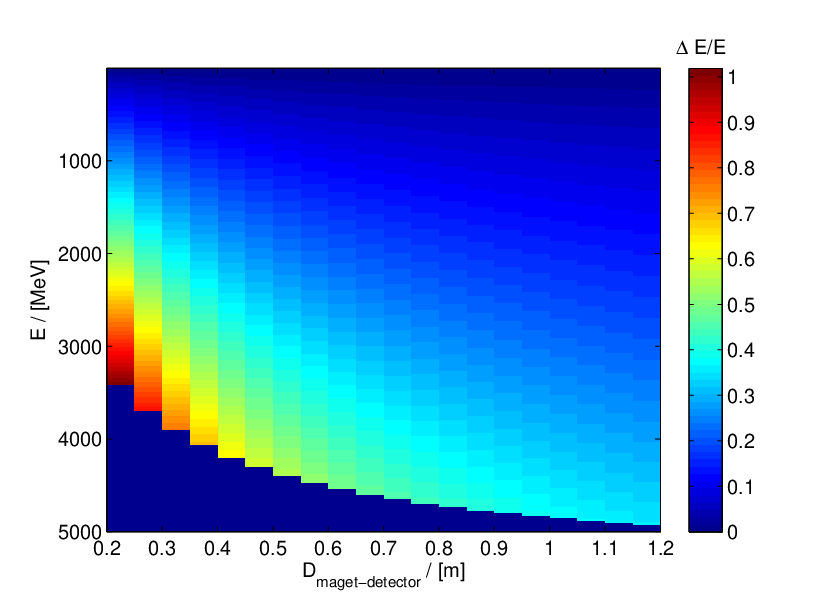

It can be seen in Fig. 4.2.1 how the focusing effect is depending on the drift length between magnet and screen. A focusing is achieved mainly on energies between 100 MeV and 200 MeV. The results shown in Fig. 4.2.1 have been made without taking space charge effects into account [4].

4.2.2 Lifting the degeneracy
However if the divergence is known the degeneracy can be lifted. Measuring the divergence can be achieved by putting a screen in front of the spectrometer (Fig. 4.2.2). This allows to measure the beam’s size and position. Now the opportunity is given to simulate the propagation of different mono energetic electron beam’s (at energy ) with the determined divergence and initial position. Once the propagation of mono energetic electron beam is known the distribution on the detection screen can be calculated easily. Since it is known how mono energetic beams map on the detection screen as a function of their energies the opportunity is given to write an arbitrary signal , which is detected on , as a linear combination of mono energetic beams .
can be fitted to the measured distribution by a root mean square method, with the restriction that for all . The set is than equal the beams energy distribution.

To get a rough understanding what influence noise at the detection screen on this analyse procedure has, a mono energetic beam with a uniform distribution in divergence (from to ) was studied. The noise was simulated by broadening the signal in y direction by . The width of the electron energy distribution was determined and uses for calculating the energy resolution (Fig. 4.2.2).

This results are only very rough estimation. The inaccuracy from the screen has not been taken in to account. Also only mono energetic beams were studied. However this maybe far from real experimental data.
4.2.3 Motion in z direction
The bulk field does not have any influence on the motion’s z component. Therefore only the stray field accelerates the particle along the z direction. Due to [3] the stray field at the magnet edge causes a defocusing in the z direction. Indeed this can be observed in the numerical simulation 4.2.3. The defocusing as a function of the energy can be simulated (Fig. 4.2.3).


However the broadening created by the magnet edge is small compared with the beam’s divergence that can be expected.
5 Conclusion
For the magnets physical properties it can be stated that the magnetic radius is . A stray field occurs over a length of . However the magnetic field’s shape does not depend on the coil current. Furthermore the maximal magnetic field was measured for different coil current and it was shown that the field is proportional to the current. In addition a memory effect for the magnetic field could be observed, depending on the path that was chosen to adjust a certain current. In the adiabatic limes the different between lowering and rising direction was found to be smaller than . For further studies it could be of interest to measure memory effects beyond the adiabatic limit.
Numerical simulation have shown how the bending angle depends on the electrons energy. It can be concluded that the bending angle does not change much for large energies (). This decreases the energy resolution dramatically for increasing energies. However at low energies the resolution is relatively high ( for ). Since some interests lies in electron energies up to a proposal has been made to resolve energy spread in this regime energies. However much more studies have to be done to clarify if this procedure is appropriated or not.
In addition focusing effects in y direction and defocusing effects in z direction has been studied. It was shown that this effects are stronger on low energies ().
6 Appendix
If it is assumed that the magnetic field is homogeneous in a circular area with radius and zero other wise (), a analytical solution for the bending angle can be found. For simplicity it is further assumed that the incident beam is perpendicular to the magnet’s surface. Symmetry reasons request that the outgoing beam is perpendicular as well. Since the magnetic field in the circular region is constant the electron’s trajectory will be a segment of a circle. The bending radius can easily be calculated by . Knowing the bending radius, the magnetic radius and the angle of incident () allows us to calculate the bending angle (see Fig.6).
The simulated results for the bending angle are plotted on a scale which shows a deviation from the analytical value as a deviation from the straight line Fig. 4.2. Even though that the analytical method gives quite good results the accuracy is not high enough.

6.1 Acknowledgment
On the experimental side the work has been supported by Ron Morton and George Hammett from the electrical work shop, Peter Shrimpton and Keith Long from the teaching facility and Mick Williams from the technical work shop at the University of Oxford.
References
- [1] W.Leemans, Nature Physics, 2 696, 2006.
- [2] K.Nakamura, Phys. Plasmas, 14 056708, 2007.
- [3] A.Banford, The transport of charged particle beams. E. & F.N. Spon Ltd., London, 1966.
- [4] S.Humphries, Charged particle beams. Wiley, New Jersey, 2002.
- [5] R.Holsinger, K.Halbach, Particle Accelerators 7, 7 213-222 1976.