跳到论文正文
W Papers独立论文阅读器 arXiv:0906.1140 论文正文 计算阅读时间 · 0%
引用这篇论文根据当前论文元数据生成,正式投稿前建议核对。


License: arXiv.org perpetual non-exclusive license
arXiv:0906.1140v1 [hep-ph] 05 Jun 2009

Leading Order QCD Shear Viscosity from the 3PI Effective Action

M.E. Carrington and E. Kovalchuk Email: carrington@brandonu.ca; kavalchuke@brandonu.ca Affiliation: Department of Physics, Brandon University, Brandon, Manitoba, R7A 6A9 Canada
and
Winnipeg Institute for Theoretical Physics, Winnipeg, Manitoba
Abstract

In this article we calculate the leading order shear viscosity in QCD using the resummed 3PI effective action. We work to 3-loop order in the effective action. We show that the integral equations that resum the pinching and collinear contributions are produced naturally by the formalism. All leading order terms are included, without the need for any kind of power counting arguments.

pacs
11.15.-q, 11.10.Wx, 05.70.Ln, 52.25.Fi

I Introduction

Transport coefficients measure the efficiency with which conserved quantities are transported through a medium, over distances that are long compared to the microscopic relaxation scales of the system (for a review see [1]). Direct applications include the early universe and the quark gluon plasma. The calculation of transport coefficients is also important from a purely theoretical standpoint. They characterize linear deviations from equilibrium, but are calculated using the familiar methods of equilibrium field theory. Results could therefore be used as a check on calculations based on purely non-equilibrium methods.

The calculation of transport coefficients in gauge theories is hugely complicated by the occurrance of pinch- and collinear-singularities [2, 3, 4]. These singularities can be regulated by using hard thermal loop propagators. However, this remedy produces infinite sets of graphs which all contribute at the same order. In order to include all leading order contributions, these infinite sets of graphs need to be resummed. The problem is to develop a technique to perform the resummation that avoids double counting and respects all of the symmetries of the original theory.

The complete leading order calculation of electrical conductivity and shear viscosity, in both QED and QCD, was done in [4]. This calculation is not obtained directly from quantum field theory, but is derived from kinetic theory. It is of interest to understand the connection between the kinetic theory approach, and a calculation based on quantum field theory. One motivation is that quantum field theory might provide a better framework than kinetic theory for calculations beyond leading order. The equivalence of the two approaches has been demonstrated for scalar theories [5, 6, 7, 8]. In QED, field theory based calculations have been done using a direct ladder summation [9, 10], dynamical remormalization group methods [11], and other diagrammatic methods [12, 13]. A large NfN_{f} leading log calculation of conductivity and shear viscosity was done in [14] using the 2PI effective theory. The conductivity has been obtained at leading order from the 3PI effective action [15, 16]. In QCD, the field theoretic calculation of shear viscosity has only been done at leading log order [9, 17]. In this paper we present the first calculation of the full leading order QCD shear viscosity using quantum field theory methods. We show that the calculation can be organized naturally using the 3PI effective action. The result provides strong support for the use of nnPI effective theories as a method to study the equilibration of quantum fields.

The nn-PI effective theory, in which the nn-point functions are treated as variational parameters, is a natural method to organize the calculation of transport coefficients. In general, a consistent resummation requires the computation of the nnPI effective action for infinite nn. However, there is an equivalence heirarchy that simplifies the structure of the calculation [18]: to 2-loop order, the infinite-PI effective action is equivalent to the 2PI effective action, to 3-loop order, the infinite-PI effective action is equivalent to the 3PI effective action, etc.

Truncations of the effective action produce problems with gauge invariance. Even though the effective action is consistent with the global symmetries of the theory, the Ward identities associated with the gauge symmetry may not be satisfied for the self consistently determined vertex functions [19, 20]. To address this problem, we use the resummed effective action, which is defined with respect to the self-consistent solutions of the nn-point functions [21, 22, 23, 24].

There are three different types of nn-point functions involved in the calculation: (1) the self-consistent solutions of the equations of motion; (2) ‘mixed’ nn-point functions obtained by taking functional derivatives of the self-consistent solutions with respect to field expectation values and; (3) ‘external’ nn-point functions obtained by taking functional derivatives of the resummed effective action with respect to field expectation values. For QED, it has been shown that the ‘external’ nn-point functions satisfy the usual Ward identities [15, 25]. At the exact level, all of these definitions are equivalent to each other. Integral equations for type (1) vertices are obtained from the equations of motion of the effective action (see Eqn. (23)). Integral equations for type (2) vertex functions are obtained by functionally differentiating the equations of motion with respect to field expectation values (see, for example, Eqn. (38)).

This paper is organized as follows. In section II we define some notation. In section III we derive an expression for the shear viscosity in terms of the integrand that gives the gluon polarization tensor. In section IV we give the 3PI effective action to 3-loop order. In section V we define some ‘external’ nn-point functions and obtain an expression for the ‘external’ 2-point function. In sections VI and VII we derive integral equations for the relevant ‘mixed’ vertices, and the self consistent vertices. In section VIII we show that the kernels of these equations can be written as the square of the sum of the amplitudes that correspond to all physical scattering and production processes. In section IX we present our conclusions. In Appendix A we define the notation used in the Keldysh representation of finite temperature field theory. In Appendix B we show that the expansion of the ‘external’ polarization tensor produced by the 3PI formalism contains all of the terms that would be produced by a Wick expansion. In Appendix C we give some details of the calculation presented in section VIII.

II Notation

We use:

g=diag⁡(1,−1,−1,−1),\displaystyle g={\rm diag}(1,-1,-1,-1)\,, (1)
nb​(p0)=1eβ​p0−1,nf​(p0)=1eβ​p0+1,\displaystyle n_{b}(p_{0})=\frac{1}{e^{\beta p_{0}}-1}\,,~~n_{f}(p_{0})=\frac{1}{e^{\beta p_{0}}+1}\,,
NB​(p0)=1+2​nb​(p0),NF​(p0)=1−2​nf​(p0),\displaystyle N_{B}(p_{0})=1+2n_{b}(p_{0})\,,~~N_{F}(p_{0})=1-2n_{f}(p_{0})\,,
∫dP:=∫d4​p(2​π)4,∫p:=∫d3​p2​Ep​(2​π)3,\displaystyle\int dP:=\int\frac{d^{4}p}{(2\pi)^{4}}\,,~~\int_{p}:=\int\frac{d^{3}p}{2E_{p}\,(2\pi)^{3}}\,,
I^i​j=(pi​pj−13​p2​δi​j)​1p2.\displaystyle\hat{I}^{ij}=\big(p^{i}p^{j}-\frac{1}{3}p^{2}\delta^{ij}\big)\,\frac{1}{p^{2}}\,.

We work in the Feynman gauge and write the QCD Lagrangian as:

ℒ=−14​Fμ​νa​Fμ​ν​a−12​(∂μAμa)2+i​ψ¯​γμ​Dμ​ψ−η¯a​∂μ(Dμ​η)a,\displaystyle{\cal L}=-\frac{1}{4}F^{a}_{\mu\nu}F^{\mu\nu~a}-\frac{1}{2}(\partial^{\mu}A_{\mu}^{a})^{2}+i\bar{\psi}\gamma_{\mu}D^{\mu}\psi-\bar{\eta}^{a}\partial^{\mu}(D_{\mu}\eta)^{a}\,, (2)
Fμ​νa=∂μAνa−∂νAμa+g​fa​b​c​Aμb​Aνc,\displaystyle F_{\mu\nu}^{a}=\partial_{\mu}A_{\nu}^{a}-\partial_{\nu}A_{\mu}^{a}+gf^{abc}A^{b}_{\mu}A^{c}_{\nu}\,,
Dμψ=(∂μ−igAμata)ψ,\displaystyle D_{\mu}\psi=(\partial_{\mu}-igA^{a}_{\mu}t^{a})\psi\,,
(Dμ​η)a=(∂μδa​c+g​fa​b​c​Aμb)​ηc.\displaystyle(D_{\mu}\eta)^{a}=\big(\partial_{\mu}\delta^{ac}+gf^{abc}A_{\mu}^{b}\big)\eta^{c}\,.

The classical action is:

Sc​l​[ψ,ψ¯,A,η,η¯]=∫d4​x​ℒ.\displaystyle S_{cl}[\psi,\bar{\psi},A,\eta,\bar{\eta}]=\int d^{4}x\,{\cal L}\,. (3)

The group factor notation for S​U​(N)SU(N) is:

fundamental​representation:\displaystyle{\rm fundamental~representation}:~~ CF=(N2−1)/(2​N),TF=1/2,dF=N,\displaystyle C_{F}=(N^{2}-1)/(2N)\,,~T_{F}=1/2\,,~d_{F}=N\,, (4)
adjoint​representation:\displaystyle{\rm adjoint~representation}:~~ CA=N,TA=N,dA=N2−1.\displaystyle C_{A}=N\,,~T_{A}=N\,,~d_{A}=N^{2}-1\,.

For simplicity we will set the coupling constant gg to one throughout.

III Shear Viscosity

The Kubo formula for shear viscosity is:

η=120​(∂∂q0​2​Im​ρπ​π​(q0,0))|q0→0\displaystyle\eta=\frac{1}{20}\left(\frac{\partial}{\partial q_{0}}2\,{\rm Im}\,\rho_{\pi\pi}(q_{0},0)\right)\Big|_{q_{0}\rightarrow 0} (5)
ρπ​π​(q0,0)=∫−∞∞d​t​∫d3​x​ei​q0​t​θ​(t)​⟨πi​j​(t,x),πi​j​(0)⟩\displaystyle\rho_{\pi\pi}(q_{0},0)=\int^{\infty}_{-\infty}dt\,\int d^{3}x\,e^{iq_{0}t}\,\theta(t)\,\langle\pi^{ij}(t,x),\pi^{ij}(0)\rangle

where πi​j\pi^{ij} is the traceless part of the energy momentum tensor.

We begin by considering the contribution to the shear viscosity that corresponds to using bare propagators and vertices. We will call this quantity η¯\bar{\eta}. We use the Keldysh representation of the real time formulation of finite temperature field theory. The basic method is described in Appendix A. The derivation of the corresponding expression for the case of the QED conductivity is given in detail in [15]. We obtain111footnotetext: Our notation throughout this paper differs slightly from that used in [15, 16]. In this paper, the symbols used to represent propagators and vertices correspond directly to lines and dots in diagrams, with no additional factors of ±i\pm i.

η¯=−110β∫dP[nf(p0)(1−nf(p0))Tr((Λ0)c​c′i​j(P+Q,Q,P)S0(P+Q)r​e​t(Λ0)c​c′i​j(P+Q,Q,P)S0(P)a​d​v)\displaystyle\bar{\eta}=-\frac{1}{10}\beta\int dP\bigg[n_{f}(p_{0})\big(1-n_{f}(p_{0})\big){\rm Tr}\bigg((\Lambda_{0})_{cc^{\prime}}^{ij}(P+Q,Q,P)S^{0}(P+Q)_{ret}\,(\Lambda_{0})_{cc^{\prime}}^{ij}(P+Q,Q,P)S^{0}(P)_{adv}\bigg) (6)
+nb​(p0)​(1+nb​(p0))​(12​(Ω0)a​bi​j​λ​τ​(−P−Q,Q,P)​Dτ​τ′0​(P+Q)r​e​t​(Ω0)a​bi​j​τ′​λ′​(−P−Q,Q,P)​Dλ​λ′0​(P)a​d​vCLOSE\displaystyle+n_{b}(p_{0})\big(1+n_{b}(p_{0})\big)\bigg(\frac{1}{2}\,(\Omega_{0})_{ab}^{ij\lambda\tau}(-P-Q,Q,P)D^{0}_{\tau\tau^{\prime}}(P+Q)_{ret}\,(\Omega_{0})^{ij\tau^{\prime}\lambda^{\prime}}_{ab}(-P-Q,Q,P)\,D^{0}_{\lambda\lambda^{\prime}}(P)_{adv}\,
−(Θ0)a​bi​j(P+Q,Q,P)G0(P+Q)r​e​t(Θ0)a​bi​j(P+Q,Q,P)G0(P)a​d​v)]q→=0q0→0\displaystyle-\,(\Theta_{0})_{ab}^{ij}(P+Q,Q,P)G^{0}(P+Q)_{ret}\,(\Theta_{0})_{ab}^{ij}(P+Q,Q,P)G^{0}(P)_{adv}\bigg)\bigg]_{\scriptsize{\begin{array}[]{l}\vec{q}=0\\ q_{0}\to 0\end{array}}}

The vertices are defined as:

(2​π)4​δ4​(K+P+Q)​(Ω0)a​bi​j​λ​τ​(K,Q,P)=∫d4​x​∫d4​y​∫d4​z​e−i​q​x​e−i​p​y​e−i​k​z​⟨Aaλ​(z)​πgluoni​j​(x)​Abτ​(y)⟩,\displaystyle(2\pi)^{4}\delta^{4}(K+P+Q)(\Omega_{0})^{ij\lambda\tau}_{ab}(K,Q,P)=\int d^{4}x\int d^{4}y\int d^{4}z\,e^{-iqx}e^{-ipy}e^{-ikz}\langle A^{\lambda}_{a}(z)\pi^{ij}_{\rm gluon}(x)A^{\tau}_{b}(y)\rangle\,, (10)
(2​π)4​δ4​(K−P−Q)​(Θ0)a​bi​j​(K,Q,P)=∫d4​x​∫d4​y​∫d4​z​e−i​q​x​e−i​p​y​ei​k​z​⟨ηa​(z)​πghosti​j​(x)​η¯b​(y)⟩,\displaystyle(2\pi)^{4}\delta^{4}(K-P-Q)(\Theta_{0})_{ab}^{ij}(K,Q,P)=\int d^{4}x\int d^{4}y\int d^{4}z\,e^{-iqx}e^{-ipy}e^{ikz}\langle\eta_{a}(z)\pi^{ij}_{\rm ghost}(x)\bar{\eta}_{b}(y)\rangle\,,
(2​π)4​δ4​(K−P−Q)​(Λ0)c​c′i​j​(K,Q,P)=∫d4​x​∫d4​y​∫d4​z​e−i​q​x​e−i​p​y​ei​k​z​⟨ψc​(z)​πquarki​j​(x)​ψ¯c′​(y)⟩,\displaystyle(2\pi)^{4}\delta^{4}(K-P-Q)(\Lambda_{0})_{cc^{\prime}}^{ij}(K,Q,P)=\int d^{4}x\int d^{4}y\int d^{4}z\,e^{-iqx}e^{-ipy}e^{ikz}\langle\psi_{c}(z)\pi^{ij}_{\rm quark}(x)\bar{\psi}_{c^{\prime}}(y)\rangle\,,

where {πquarki​j,πghosti​j,πgluoni​j}\{\pi^{ij}_{\rm quark},~\pi^{ij}_{\rm ghost},~\pi^{ij}_{\rm gluon}\} indicates the part of the traceless energy momentum tensor that is quadratic in quark, ghost, and gluon fields. For the ghost and quark vertices the order of the momenta is: outgoing momentum of the outgoing ghost/quark, incoming momentum of the gluon, incoming momentum of the incoming ghost/quark. For the gluon vertex all momenta are incoming.

The integral in (6) contains three bubble-type diagrams: a gluon bubble, a ghost bubble, and a quark bubble. These diagrams contain pinching and collinear singularities that need to be resummed in order to obtain the full leading order contribution. In order to simplify the explanation of this point, we consider a generic bubble diagram, and draw the propagators as solid lines, as shown in Fig. 1. Throughout this paper we will use stars to indicate the legs of a type (2) or type (3) nn-point function that correspond to functional derivatives with respect to field expectation values (see also Fig. 6).

Refer to caption
Figure 1: A generic contribution to the shear viscosity.

Pinch singularities are produced by the low frequency limit in the Kubo formula (Eqn. (5)). When integrating a term of the form ∫d​p0​Gr​e​t​(P)​Ga​d​v​(P)\int dp_{0}\;G^{ret}(P)G^{adv}(P), the integration contour is ‘pinched’ between poles on each side of the real axis, and the integral contains a divergence called a ‘pinch singularity.’ A set of graphs containing pinch singularities has the general form shown in Fig. 2.

Refer to caption
Figure 2: Contributions to the shear viscosity from pinching singularities.

In gauge theories, one also has collinear singularities. Fig. 3 shows a set of graphs with collinear singularities.

Refer to caption
Figure 3: Contributions to the shear viscosity from collinear singularities.

In general, pinch and collinear singularities are regulated by using hard thermal loop (HTL) resummed propagators. This procedure introduces extra factors of the coupling in the denominators which change the power counting. As a consequence, the infinite series of graphs depicted in Figs. 2 and 3 are all of the same order and need to be resummed. The resummation is done by solving a set of coupled integral equations that have the general form shown in Fig. 4. When the leg on the right hand side has a star, the integral equation resums pinch singularities. The same equation without the star resums collinear singularities. The basic goal of this paper is to show that these integral equations are produced naturally by the 3PI formalism. We note that since the ghost HTL self energy is zero, the ghost diagram cannot be regulated in this way. However, ghosts are not physical particles and are only needed to cancel unphysical gluon polarizations. We will show explicitly how this works in section VIII.

Refer to caption
Figure 4: An integral equation that resums singularities.

In Feynman gauge the HTL quark, ghost and gluon propagators can be written:

−i​S​(P)=1P/−Σ,−i​Ga​b​(P)=δa​bP2,\displaystyle-iS(P)=\frac{1}{P\!\!\!\!/~-\Sigma}\,,~~-iG_{ab}(P)=\frac{\delta_{ab}}{P^{2}}\,, (11)
Da​bμ​ν​(P)=δa​b​Dμ​ν​(P),−i​Dμ​ν​(P)=−PTμ​ν​1P2−ΠT−PLμ​ν​1P2−ΠL−PGμ​ν​1P2,\displaystyle D_{ab}^{\mu\nu}(P)=\delta_{ab}D^{\mu\nu}(P)\,,~~-iD^{\mu\nu}(P)=-P_{T}^{\mu\nu}\frac{1}{P^{2}-\Pi_{T}}-P_{L}^{\mu\nu}\frac{1}{P^{2}-\Pi_{L}}-P_{G}^{\mu\nu}\frac{1}{P^{2}}\,,
PTμ​ν=gμ​ν−Uμ​Uν+(Pμ−p0​Uμ)​(Pν−p0​Uν)/p2;U=(1,0,0,0),\displaystyle P_{T}^{\mu\nu}=g^{\mu\nu}-U^{\mu}U^{\nu}+(P^{\mu}-p_{0}U^{\mu})(P^{\nu}-p_{0}U^{\nu})/p^{2}\,;~~U=(1,0,0,0)\,,
PLμ​ν=−PTμ​ν+gμ​ν−Pμ​Pν/P2,PGμ​ν=Pμ​Pν/P2.\displaystyle P_{L}^{\mu\nu}=-P_{T}^{\mu\nu}+g^{\mu\nu}-P^{\mu}P^{\nu}/P^{2}\,,~~P_{G}^{\mu\nu}=P^{\mu}P^{\nu}/P^{2}\,.

Dominant contributions to the shear viscosity come from hard excitations on the pinching lines, and the residue of the longtitudinal part of the gluon propagator is exponentially suppressed at high temperatures. Therefore, we need only the transverse part of the pinching gluon propagator which can be written:

−i​DTi​j​(P)=(δi​j−pi​pjp2)​1P2−ΠT.\displaystyle-iD^{ij}_{T}(P)=\big(\delta^{ij}-\frac{p^{i}p^{j}}{p^{2}}\big)\frac{1}{P^{2}-\Pi_{T}}\,. (12)

Now we consider the vertices defined in (10). We factor the colour structure by defining:

(Ω0)a​bi​j​λ​τ=δa​b​Ω0i​j​λ​τ,(Θ0)a​bi​j=δa​b​Θ0i​j,(Λ0)c​c′i​j=δc​c′​Λ0i​j.\displaystyle(\Omega_{0})_{ab}^{ij\lambda\tau}=\delta_{ab}\Omega_{0}^{ij\lambda\tau}\,,~~(\Theta_{0})_{ab}^{ij}=\delta_{ab}\Theta_{0}^{ij}\,,~~(\Lambda_{0})_{cc^{\prime}}^{ij}=\delta_{cc^{\prime}}\Lambda_{0}^{ij}\,. (13)

In addition, we write the bare vertices that are obtained directly from the Lagrangian as:

(Ω0)a​c​bλ​σ​τ​(−P,0,P)=fa​c​b​Ω0λ​σ​τ​(−P,0,P),\displaystyle(\Omega_{0})^{\lambda\sigma\tau}_{acb}(-P,0,P)=f_{acb}\Omega_{0}^{\lambda\sigma\tau}(-P,0,P)\,, (14)
(Θ0)a​c​bσ​(P,0,P)=fa​c​b​Θ0σ​(P,0,P),\displaystyle(\Theta_{0})^{\sigma}_{acb}(P,0,P)=f_{acb}\Theta_{0}^{\sigma}(P,0,P)\,,
(Λ0)c​c′​(P,0,P)=δc​c′​Λ0​(P,0,P).\displaystyle(\Lambda_{0})_{cc^{\prime}}(P,0,P)=\delta_{cc^{\prime}}\Lambda_{0}(P,0,P)\,.

Note that we have used the same letters in (10) and (14). In order to simplify the notation, we do not introduce any additional primes or tildes to distinguish the two types of vertices. The indices associated with each vertex are sufficient to indicate which type of vertex is meant. Using this notation, it is straightforward to show that:

Ωλ​τ;i​j​(−P,0,P)→2​gλ​τ​p2​I^i​j→ps​Ωλ​s​τ​(−P,0,P)​I^i​j,\displaystyle\Omega^{\lambda\tau;ij}(-P,0,P)~~\rightarrow~~2g^{\lambda\tau}p^{2}\hat{I}^{ij}~~\rightarrow~~p^{s}\Omega^{\lambda s\tau}(-P,0,P)\hat{I}^{ij}\,, (15)
Θ0i​j​(P,0,P)=−p2​I^i​j=ps​Θ0s​(P,0,P)​I^i​j,\displaystyle\Theta_{0}^{ij}(P,0,P)=-p^{2}\hat{I}^{ij}=p^{s}\Theta^{s}_{0}(P,0,P)\hat{I}^{ij}\,,
Λi​j​(P,0,P)=13​δi​j​pl​γl−γi​pj,\displaystyle\Lambda^{ij}(P,0,P)=\frac{1}{3}\delta^{ij}p^{l}\gamma^{l}-\gamma^{i}p^{j}\,,

where the arrow indicates that the relation holds only when multiplied by the transverse projectors PTλ​λ′​PTτ​τ′P_{T}^{\lambda\lambda^{\prime}}P_{T}^{\tau\tau^{\prime}} on both sides. We have taken the limit Q→0Q\to 0, since this produces no difficulties for factors in the numerator of the integrand.

Using these results we can rewrite the integrand in (6) in terms of the integrand for the gluon self energy. We separate contributions to the gluon self energy from gluon, ghost and quark bubbles by writing:

Π​[i]a​bs​s′​(Q)=∫d​P​Π​i​n​t​[i]a​bs​s′​(P,Q);i∈{gluon,ghost,quark}.\displaystyle\Pi[i]^{ss^{\prime}}_{ab}(Q)=\int dP\,\Pi int[i]^{ss^{\prime}}_{ab}(P,Q)\,;~~~i\in\{{\rm gluon},~{\rm ghost},~{\rm quark}\}\,. (16)

It is straightforward to show that (6) can be written:

η¯=\displaystyle\bar{\eta}= β10​I^2​δa​b​∫d​P​ps​ps′\displaystyle\frac{\beta}{10}\hat{I}^{2}\delta_{ab}\int dP\,p^{s}\,p^{s^{\prime}}\, (17)
⋅(1CA​(Π​i​n​t​[gluon]a​bs​s′​(P,Q)+Π​i​n​t​[ghost]a​bs​s′​(P,Q))+NcdA​TF​Π​i​n​t​[quark]a​bs​s′​(P,Q))|q→=0q0→0\displaystyle\cdot\;\bigg(\frac{1}{C_{A}}\big(\Pi int[{\rm gluon}]^{ss^{\prime}}_{ab}(P,Q)+\Pi int[{\rm ghost}]^{ss^{\prime}}_{ab}(P,Q)\big)+\frac{N_{c}}{d_{A}T_{F}}\Pi int[{\rm quark}]^{ss^{\prime}}_{ab}(P,Q)\bigg)\bigg|_{\scriptsize{\begin{array}[]{l}\vec{q}=0\\ q_{0}\to 0\end{array}}}

IV The 3PI formalism

At this point, we introduce a compactified notation. We use a single numerical subscript to represent all continuous and discrete indices. For example: a gluon field is written A1:=Aμa​(x)A_{1}:=A^{a}_{\mu}(x); the quark propagator is written S12:=Sα​β​(x1,x2)S_{12}:=S_{\alpha\beta}(x_{1},x_{2}); the bare 3-gluon vertex is written Ω1320:=(Ω0)a​c​bλ​σ​τ​(x1,x3,x2)\Omega^{0}_{132}:=(\Omega_{0})^{\lambda\sigma\tau}_{acb}(x_{1},x_{3},x_{2}) etc. We also use an Einstein convention in which a repeated index implies a sum over discrete variables and an integration over space-time variables. The free propagators and vertices are defined as:

(S120)−1=−i​δ2​Sc​lδ​ψ2​δ​ψ¯1,(D120)−1=−i​δ2​Sc​lδ​A2​δ​A1,(G120)−1=−i​δ2​Sc​lδ​η2​δ​η¯1,\displaystyle(S^{0}_{12})^{-1}=-i\frac{\delta^{2}S_{cl}}{\delta\psi_{2}\delta\bar{\psi}_{1}}\,,~~(D^{0}_{12})^{-1}=-i\frac{\delta^{2}S_{cl}}{\delta A_{2}\delta A_{1}}\,,~~(G^{0}_{12})^{-1}=-i\frac{\delta^{2}S_{cl}}{\delta\eta_{2}\delta\bar{\eta}_{1}}\,, (21)
Λ1320=i​δ3​Sc​lδ​ψ2​δ​A3​δ​ψ¯1=−δ​(S120)−1δ​A3,Ω1320=i​δ3​Sc​lδ​A2​δ​A3​δ​A1=−δ​(D120)−1δ​A3,\displaystyle\Lambda^{0}_{132}=i\frac{\delta^{3}S_{cl}}{\delta\psi_{2}\delta A_{3}\delta\bar{\psi}_{1}}=-\frac{\delta(S^{0}_{12})^{-1}}{\delta A_{3}}\,,~~\Omega^{0}_{132}=i\frac{\delta^{3}S_{cl}}{\delta A_{2}\delta A_{3}\delta A_{1}}=-\frac{\delta(D^{0}_{12})^{-1}}{\delta A_{3}}\,,
Θ1320=i​δ3​Sc​lδ​η2​δ​A3​δ​η¯1=−δ​(G120)−1δ​A3,M12340=i​δ4​Sc​lδ​A4​δ​A3​δ​A2​δ​A1=δ​Ω1320δ​A4=−δ2​(D120)−1δ​A4​δ​A3.\displaystyle\Theta^{0}_{132}=i\frac{\delta^{3}S_{cl}}{\delta\eta_{2}\delta A_{3}\delta\bar{\eta}_{1}}=-\frac{\delta(G^{0}_{12})^{-1}}{\delta A_{3}}\,,~~M^{0}_{1234}=i\frac{\delta^{4}S_{cl}}{\delta A_{4}\delta A_{3}\delta A_{2}\delta A_{1}}=\frac{\delta\Omega_{132}^{0}}{\delta A_{4}}=-\frac{\delta^{2}(D^{0}_{12})^{-1}}{\delta A_{4}\delta A_{3}}\,.

The 3PI effective action can be written [18, 26]:

Γ⁡[ψ,ψ¯,A,η,η¯,S,D,G,V,U,Y]=Sc​l​[ψ,ψ¯,A,η,η¯]\displaystyle\Gamma[\psi,\bar{\psi},A,\eta,\bar{\eta},S,D,G,V,U,Y]=S_{cl}[\psi,\bar{\psi},A,\eta,\bar{\eta}] (22)
+i2​Tr​Ln​D12−1+i2​Tr​[(D120)−1​(D21−D210)]−i​Tr​Ln​S12−1−i​Tr​[(S120)−1​(S21−S210)]\displaystyle~~~~+\frac{i}{2}{\rm Tr}\,{\rm Ln}D^{-1}_{12}+\frac{i}{2}{\rm Tr}\left[(D^{0}_{12})^{-1}\left(D_{21}-D^{0}_{21}\right)\right]-i{\rm Tr}\,{\rm Ln}S^{-1}_{12}-i{\rm Tr}\left[(S^{0}_{12})^{-1}(S_{21}-S^{0}_{21})\right]
−i​Tr​Ln​G12−1−i​Tr​[(G120)−1​(G21−G210)]+Γ0​[A,S,D,G,V,U,Y]+Γint​[A,S,D,G,V,U,Y].\displaystyle~~~~-i{\rm Tr}\,{\rm Ln}G^{-1}_{12}-i{\rm Tr}\left[(G^{0}_{12})^{-1}(G_{21}-G^{0}_{21})\right]+\Gamma^{0}[A,S,D,G,V,U,Y]+\Gamma^{\rm int}[A,S,D,G,V,U,Y]\,.

We use the following notation: VV is the self consistent quark-gluon vertex, UU is the self consistent 3-gluon vertex, and YY is the self consistent ghost-gluon vertex. These propagators and vertices are to be determined self-consistently from the equations of motion. We also define Φ=i⁡(Γ0+Γint)\Phi=i(\Gamma^{0}+\Gamma^{\rm int}). We show Φ\Phi graphically in Fig. 5. We note that shifting the field introduces another 3-point vertex and that, in the figure, the intersection of three gluon lines at a small dot represents Ωi​j​k0+Al​Mi​j​k​l0\Omega_{ijk}^{0}+A_{l}M_{ijkl}^{0}.

Refer to caption
Figure 5: The 3-loop 3PI effective action. Wiggly lines represent gluons, solid lines are quarks and dotted lines are ghosts.

The equations of motion are obtained from the stationarity of the action. There are 11 equations which are obtained by functionally differentiating with respect to the 11 functional arguments of the effective action:

δ​Γδ​Xi=0;Xi∈{ψ,ψ¯,A,η,η¯,S,D,G,U,V,Y}.\displaystyle\frac{\delta\Gamma}{\delta X_{i}}=0\,;~~~~X_{i}\in\{\psi,\bar{\psi},A,\eta,\bar{\eta},S,D,G,U,V,Y\}\,. (23)

The equations obtained by varying with respect to {S,D,G,U,V,Y}\{S,D,G,U,V,Y\} can be solved simultaneously for the self consistent solutions which are functions of the field expectation values: S~​[ψ,ψ¯,A,η,η¯]\tilde{S}[\psi,\bar{\psi},A,\eta,\bar{\eta}], D~​[ψ,ψ¯,A,η,η¯]\tilde{D}[\psi,\bar{\psi},A,\eta,\bar{\eta}], G~​[ψ,ψ¯,A,η,η¯]\tilde{G}[\psi,\bar{\psi},A,\eta,\bar{\eta}], U~​[ψ,ψ¯,A,η,η¯]\tilde{U}[\psi,\bar{\psi},A,\eta,\bar{\eta}], V~​[ψ,ψ¯,A,η,η¯]\tilde{V}[\psi,\bar{\psi},A,\eta,\bar{\eta}], Y~​[ψ,ψ¯,A,η,η¯]\tilde{Y}[\psi,\bar{\psi},A,\eta,\bar{\eta}]. We write this set of self consistent solutions:

X~={S~,D~,G~,U~,V~,Y~}.\displaystyle\tilde{X}=\{\tilde{S},\tilde{D},\tilde{G},\tilde{U},\tilde{V},\tilde{Y}\}\,. (24)

Substituting these self consistent solutions we obtain the resummed action, which depends only on the expectation values of the fields:

Γ~​[ψ,ψ¯,A,η,η¯]\displaystyle\tilde{\Gamma}[\psi,\bar{\psi},A,\eta,\bar{\eta}] (25)
=Γ⁡[ψ,ψ¯,A,S~​[ψ,ψ¯,A,η,η¯],D~​[ψ,ψ¯,A,η,η¯],G~​[ψ,ψ¯,A,η,η¯],V~​[ψ,ψ¯,A,η,η¯],U~​[ψ,ψ¯,A,η,η¯],Y~​[ψ,ψ¯,A,η,η¯]].\displaystyle=\Gamma[\psi,\bar{\psi},A,\tilde{S}[\psi,\bar{\psi},A,\eta,\bar{\eta}],\tilde{D}[\psi,\bar{\psi},A,\eta,\bar{\eta}],\tilde{G}[\psi,\bar{\psi},A,\eta,\bar{\eta}],\tilde{V}[\psi,\bar{\psi},A,\eta,\bar{\eta}],\tilde{U}[\psi,\bar{\psi},A,\eta,\bar{\eta}],\tilde{Y}[\psi,\bar{\psi},A,\eta,\bar{\eta}]]\,.

The equivalence of (22) and (25) at the exact level was shown in [27]. In the future we will write Γ\Gamma and Γ~\tilde{\Gamma} without their arguments.

V ‘External’ nn-point functions

We define some type (2) ‘mixed’ vertex functions using the same notation as (21):

Ω132=−δ​D~12−1δ​A3,Θ132=−δ​G~12−1δ​A3,Λ132=−δ​S~12−1δ​A3.\displaystyle\Omega_{132}=-\frac{\delta\tilde{D}^{-1}_{12}}{\delta A_{3}}\,,~~\Theta_{132}=-\frac{\delta\tilde{G}^{-1}_{12}}{\delta A_{3}}\,,~~\Lambda_{132}=-\frac{\delta\tilde{S}^{-1}_{12}}{\delta A_{3}}\,. (26)

These vertices are shown in Fig. 6. ‘External’ gluon legs are distinguished by a star.

Refer to caption
Figure 6: Some ‘mixed’ vertices.

Some additional useful relations can be obtained from the identities:

D~13−1​D~32=δ12,G~13−1​G~32=δ12,S~13−1​S~32=δ12.\displaystyle\tilde{D}^{-1}_{13}\tilde{D}_{32}=\delta_{12}\,,~~\tilde{G}^{-1}_{13}\tilde{G}_{32}=\delta_{12}\,,~~\tilde{S}^{-1}_{13}\tilde{S}_{32}=\delta_{12}\,. (27)

Differentiating (27) with respect to AA and using (26) gives:

δ​D~12δ​A3=D~11′​Ω1′​32′​D~2′​2,δ​G~12δ​A3=G~11′​Φ1′​32′​G~2′​2,δ​S~12δ​A3=S~11′​Λ1′​32′​S~2′​2.\displaystyle\frac{\delta\tilde{D}_{12}}{\delta A_{3}}=\tilde{D}_{11^{\prime}}\Omega_{1^{\prime}32^{\prime}}\tilde{D}_{2^{\prime}2}\,,~~\frac{\delta\tilde{G}_{12}}{\delta A_{3}}=\tilde{G}_{11^{\prime}}\Phi_{1^{\prime}32^{\prime}}\tilde{G}_{2^{\prime}2}\,,~~\frac{\delta\tilde{S}_{12}}{\delta A_{3}}=\tilde{S}_{11^{\prime}}\Lambda_{1^{\prime}32^{\prime}}\tilde{S}_{2^{\prime}2}\,. (28)

The ‘external’ gluon propagator is defined as:

i​(D12ext)−1=δ2δ​A2​δ​A1​Γ~​[ψ,ψ¯,A,η¯,η].\displaystyle i(D^{{\rm ext}}_{12})^{-1}=\frac{\delta^{2}}{\delta A_{2}\delta A_{1}}\tilde{\Gamma}[\psi,\bar{\psi},A,\bar{\eta},\eta]\,. (29)

The ‘external’ self energy is extracted from the ‘external’ propagator using:

(D12ext)−1=(D120)−1−Π12ext.\displaystyle(D^{{\rm ext}}_{12})^{-1}=(D^{0}_{12})^{-1}-\Pi^{\rm ext}_{12}\,. (30)

We can derive an expression for the ‘external’ self energy as a function of the vertices in (26) by taking derivatives of the modified effective action and using the chain rule. We use the notation XiX_{i} to indicate one of the set of functional variables X:={S,D,G,V,U,Y}X:=\{S,D,G,V,U,Y\} and X~i\tilde{X}_{i} to indicate one of the set of self-consistent solutions X~:={S~,D~,G~,V~,U~,Y~}\tilde{X}:=\{\tilde{S},\tilde{D},\tilde{G},\tilde{V},\tilde{U},\tilde{Y}\}. We obtain:

i​(D12ext)−1\displaystyle i(D^{{\rm ext}}_{12})^{-1} (31)
=δ2​Γδ​A2​δ​A1|X~+∑iδ​Γδ​Xi|X~​δ2​X~iδ​A1​δ​A2+[∑iδ2​Γδ​Xi​δ​A1|X~​δ​X~iδ​A2+{1↔2}]+∑i∑jδ2​Γδ​Xi​δ​Xj|X~​δ​X~iδ​A1​δ​X~jδ​A2.\displaystyle=\frac{\delta^{2}\Gamma}{\delta A_{2}\delta A_{1}}\Big|_{\tilde{X}}+\sum_{i}\frac{\delta\Gamma}{\delta X_{i}}\Big|_{\tilde{X}}\frac{\delta^{2}\tilde{X}_{i}}{\delta A_{1}\delta A_{2}}+\Big[\sum_{i}\frac{\delta^{2}\Gamma}{\delta X_{i}\delta A_{1}}\Big|_{\tilde{X}}\frac{\delta\tilde{X}_{i}}{\delta A_{2}}~+~\{1\leftrightarrow 2\}\Big]+\sum_{i}\sum_{j}\frac{\delta^{2}\Gamma}{\delta X_{i}\delta X_{j}}\Big|_{\tilde{X}}\frac{\delta\tilde{X}_{i}}{\delta A_{1}}\frac{\delta\tilde{X}_{j}}{\delta A_{2}}\,.

The second term in this result is identically zero (see Eqn. (23)). The expression can be further simplified by using the set of equations obtained by differentiating the equations of motion:

δδ​A2​[δ​Γδ​Xi|X~]=0⇒δ2​Γδ​Xi​δ​A2|X~+∑jδ2​Γδ​Xj​δ​Xi|X~​δ​X~jδ​A2=0.\displaystyle\frac{\delta}{\delta A_{2}}\;\Big[\frac{\delta\Gamma}{\delta X_{i}}\Big|_{\tilde{X}}\Big]=0~~\Rightarrow~~\frac{\delta^{2}\Gamma}{\delta X_{i}\delta A_{2}}\Big|_{\tilde{X}}+\sum_{j}\frac{\delta^{2}\Gamma}{\delta X_{j}\delta X_{i}}\Big|_{\tilde{X}}\frac{\delta\tilde{X}_{j}}{\delta A_{2}}=0\,. (32)

Using this constraint (31) becomes:

i​(D12ext)−1=δ2​Γδ​A2​δ​A1|X~+∑iδ2​Γδ​Xi​δ​A1|X~​δ​X~iδ​A2.\displaystyle i(D^{{\rm ext}}_{12})^{-1}=\frac{\delta^{2}\Gamma}{\delta A_{2}\delta A_{1}}\Big|_{\tilde{X}}+\sum_{i}\frac{\delta^{2}\Gamma}{\delta X_{i}\delta A_{1}}\Big|_{\tilde{X}}\frac{\delta\tilde{X}_{i}}{\delta A_{2}}\,. (33)

Expanding the sum and using (28) we have:

i​(D12ext)−1=δ2​Γδ​A2​δ​A1|X~\displaystyle i(D^{{\rm ext}}_{12})^{-1}=\frac{\delta^{2}\Gamma}{\delta A_{2}\delta A_{1}}\Big|_{\tilde{X}} (34)
+δ2​Γδ​S34​δ​A1|X~⋅(S~33′Λ3′​24′S~4′​4)+δ2​Γδ​D34​δ​A1|X~⋅(D~33′Ω3′​24′D~4′​4)+δ2​Γδ​G34​δ​A1|X~⋅(G~33′Θ3′​24′G~4′​4)\displaystyle~~+\frac{\delta^{2}\Gamma}{\delta S_{34}\delta A_{1}}\Big|_{\tilde{X}}\cdot(\tilde{S}_{33^{\prime}}\Lambda_{3^{\prime}24^{\prime}}\tilde{S}_{4^{\prime}4})+\frac{\delta^{2}\Gamma}{\delta D_{34}\delta A_{1}}\Big|_{\tilde{X}}\cdot(\tilde{D}_{33^{\prime}}\Omega_{3^{\prime}24^{\prime}}\tilde{D}_{4^{\prime}4})+\frac{\delta^{2}\Gamma}{\delta G_{34}\delta A_{1}}\Big|_{\tilde{X}}\cdot(\tilde{G}_{33^{\prime}}\Theta_{3^{\prime}24^{\prime}}\tilde{G}_{4^{\prime}4})
+δ2​Γδ​U345​δ​A1|X~​δ​U~345δ​A2+δ2​Γδ​V345​δ​A1|X~​δ​V~345δ​A2+δ2​Γδ​Y345​δ​A1|X~​δ​Y~345δ​A2.\displaystyle~~+\frac{\delta^{2}\Gamma}{\delta U_{345}\delta A_{1}}\Big|_{\tilde{X}}\frac{\delta\tilde{U}_{345}}{\delta A_{2}}+\frac{\delta^{2}\Gamma}{\delta V_{345}\delta A_{1}}\Big|_{\tilde{X}}\frac{\delta\tilde{V}_{345}}{\delta A_{2}}+\frac{\delta^{2}\Gamma}{\delta Y_{345}\delta A_{1}}\Big|_{\tilde{X}}\frac{\delta\tilde{Y}_{345}}{\delta A_{2}}\,.

Using (22) we obtain:

−i​δ2δ​A2​δ​A1​Γ=(D120)−1−12​M13420​D43−δ2​Φδ​A2​δ​A1\displaystyle-i\frac{\delta^{2}}{\delta A_{2}\delta A_{1}}\Gamma=(D^{0}_{12})^{-1}-\frac{1}{2}M^{0}_{1342}\,D_{43}-\frac{\delta^{2}\Phi}{\delta A_{2}\delta A_{1}} (35)
−iδ2​Γδ​S34​δ​A1|X~⋅(S~33′Λ3′​24′S~4′​4)=(Λ0−δ2​Φδ​S​δ​A)413⋅(S~ΛS~)324\displaystyle-i\frac{\delta^{2}\Gamma}{\delta S_{34}\delta A_{1}}\Big|_{\tilde{X}}\cdot(\tilde{S}_{33^{\prime}}\Lambda_{3^{\prime}24^{\prime}}\tilde{S}_{4^{\prime}4})=\bigg(\Lambda_{0}-\frac{\delta^{2}\Phi}{\delta S\,\delta A}\bigg)_{413}\cdot(\tilde{S}\Lambda\tilde{S})_{324}
−iδ2​Γδ​D34​δ​A1|X~⋅(D~33′Ω3′​24′D~4′​4)=−12(Ω0+2δ2​Φδ​D​δ​A)413⋅(D~ΩD~)324\displaystyle-i\frac{\delta^{2}\Gamma}{\delta D_{34}\delta A_{1}}\Big|_{\tilde{X}}\cdot(\tilde{D}_{33^{\prime}}\Omega_{3^{\prime}24^{\prime}}\tilde{D}_{4^{\prime}4})=-\frac{1}{2}\bigg(\Omega_{0}+2\frac{\delta^{2}\Phi}{\delta D\,\delta A}\bigg)_{413}\cdot(\tilde{D}\Omega\tilde{D})_{324}
−iδ2​Γδ​G34​δ​A1|X~⋅(G~33′Θ3′​24′G~4′​4)=(Θ0−δ2​Φδ​G​δ​A)413⋅(G~ΘG~)324.\displaystyle-i\frac{\delta^{2}\Gamma}{\delta G_{34}\delta A_{1}}\Big|_{\tilde{X}}\cdot(\tilde{G}_{33^{\prime}}\Theta_{3^{\prime}24^{\prime}}\tilde{G}_{4^{\prime}4})=\bigg(\Theta_{0}-\frac{\delta^{2}\Phi}{\delta G\,\delta A}\bigg)_{413}\cdot(\tilde{G}\Theta\tilde{G})_{324}\,.

The last three terms in (34) do not contribute because the derivatives δ​U~/δ​A\delta\tilde{U}/\delta A, δ​V~/δ​A\delta\tilde{V}/\delta A, δ​Y~/δ​A\delta\tilde{Y}/\delta A correspond to effective 4-point vertices, which are not part of our leading order calculation. We extract Π12ext\Pi_{12}^{\rm ext} from (30), (34) and (35):

Π12ext\displaystyle\Pi_{12}^{\rm ext} =12​M13420​D43+12​(Ω0+2​δ2​Φδ​D​δ​A)413⋅(D~​Ω​D~)324−(Λ0−δ2​Φδ​S​δ​A)413⋅(S~​Λ​S~)324\displaystyle=\frac{1}{2}M^{0}_{1342}\,D_{43}+\frac{1}{2}\bigg(\Omega_{0}+2\frac{\delta^{2}\Phi}{\delta D\,\delta A}\bigg)_{413}\cdot(\tilde{D}\Omega\tilde{D})_{324}-\bigg(\Lambda_{0}-\frac{\delta^{2}\Phi}{\delta S\,\delta A}\bigg)_{413}\cdot(\tilde{S}\Lambda\tilde{S})_{324} (36)
−(Θ0−δ2​Φδ​G​δ​A)413⋅(G~ΘG~)324+δ2​Φδ​A2​δ​A1.\displaystyle-\bigg(\Theta_{0}-\frac{\delta^{2}\Phi}{\delta G\,\delta A}\bigg)_{413}\cdot(\tilde{G}\Theta\tilde{G})_{324}+\frac{\delta^{2}\Phi}{\delta A_{2}\delta A_{1}}\,.

The terms in round brackets can be written collectively using the notation:

Ω0′:=(Ω0+2​δ2​Φδ​D​δ​A),Λ0′:=(Λ0−δ2​Φδ​S​δ​A),Θ0′:=(Θ0−δ2​Φδ​G​δ​A).\displaystyle\Omega^{\prime}_{0}:=\bigg(\Omega_{0}+2\frac{\delta^{2}\Phi}{\delta D\,\delta A}\bigg)\,,~~\Lambda^{\prime}_{0}:=\bigg(\Lambda_{0}-\frac{\delta^{2}\Phi}{\delta S\,\delta A}\bigg)\,,~~\Theta^{\prime}_{0}:=\bigg(\Theta_{0}-\frac{\delta^{2}\Phi}{\delta G\,\delta A}\bigg)\,. (37)

The result for the ‘external’ self energy in (36) is shown in Fig. 7. The open circles in the figure denote Ω0′\Omega_{0}^{\prime}, Λ0′\Lambda_{0}^{\prime} and Θ0′\Theta_{0}^{\prime}, and the solid dots are Ω\Omega, Λ\Lambda and Θ\Theta.

Refer to caption
Figure 7: The ‘external’ self-energy.

The last term in Fig. 7 can be calculated using the expression for Φ\Phi shown in Fig. 5. The result is shown in Fig. 8.

Refer to caption
Figure 8: A contribution to the conductivity.

In order to calculate the viscosity using the 3PI formalism we use Eqn. (17), with the integrands for the pieces Π​i​n​t​[gluon]a​bs​s′​(K,Q)\Pi int[{\rm gluon}]^{ss^{\prime}}_{ab}(K,Q), Π​i​n​t​[quark]a​bs​s′​(K,Q)\Pi int[{\rm quark}]^{ss^{\prime}}_{ab}(K,Q) and Π​i​n​t​[ghost]a​bs​s′\Pi int[{\rm ghost}]^{ss^{\prime}}_{ab} given by the 2nd, 3rd and 4th terms in (36), which are shown in the 2nd, 3rd and 4th diagrams in Fig. 7. The vertices Ω\Omega, Θ\Theta and Λ\Lambda, and the self consistent vertices UU, VV and YY, satisfy a set of coupled integral equations that resum the pinching and collinear singularities. In the next two sections we derive these integral equations.

In most cases, the equations in this paper are easier to understand when represented diagramatically. From this point on, we will give most results only as diagrams. When equations are used, all indices are suppressed.

VI Integral Equations for ‘Mixed’ Vertex Functions

In this section we derive the integral equations for the type (2) ‘mixed’ vertex functions Ω\Omega, Λ\Lambda and Θ\Theta that appear in the bubble diagrams in Πext\Pi^{\rm ext} (see Fig. 7). As explained earlier, these equations are obtained by taking functional derivatives with respect to the field expectation values of the appropriate equations of motion (23).

The integral equation for the vertex Ω\Omega is obtained from the equation:

δδ​A​[δ​Γδ​D|X~]=0.\displaystyle\frac{\delta}{\delta A}\bigg[\frac{\delta\Gamma}{\delta D}\bigg|_{\tilde{X}}\bigg]=0\,. (38)

The subscript X~\tilde{X} indicates that all self consistent solutions (24) are substituted. Using (22) and (26) it is straightforward to show that this expression can be written:

Ω=Ω0′+2​∑iδ​X~iδ​A​[δ2​Φδ​D​δ​Xi|X~],\displaystyle\Omega=\Omega_{0}^{\prime}+2\sum_{i}\frac{\delta\tilde{X}_{i}}{\delta A}\,\bigg[\frac{\delta^{2}\,\Phi}{\delta D\,\delta X_{i}}\bigg|_{\tilde{X}}\bigg]\,, (39)

where the summation indicates contributions from all of the terms in the set {S,D,G,V,U,Y}\{S,D,G,V,U,Y\}. The terms Xi∈{U,V,Y}X_{i}\in\{U,V,Y\} give no contribution, because the derivatives δ​X~i/δ​A\delta\tilde{X}_{i}/\delta A correspond to effective 4-point vertices, which are not part of the leading order calculation. Expanding the sum we have:

Ω=Ω0′+2​δ​D~δ​A​[δ2​Φδ​D​δ​D|X~]+2​δ​S~δ​A​[δ2​Φδ​D​δ​S|X~]+2​δ​G~δ​A​[δ2​Φδ​D​δ​G|X~].\displaystyle\Omega=\Omega^{\prime}_{0}+2\frac{\delta\tilde{D}}{\delta A}\,\bigg[\frac{\delta^{2}\,\Phi}{\delta D\delta D}\bigg|_{\tilde{X}}\bigg]+2\frac{\delta\tilde{S}}{\delta A}\,\bigg[\frac{\delta^{2}\,\Phi}{\delta D\,\delta S}\bigg|_{\tilde{X}}\bigg]+2\frac{\delta\tilde{G}}{\delta A}\,\bigg[\frac{\delta^{2}\,\Phi}{\delta D\,\delta G}\bigg|_{\tilde{X}}\bigg]\,. (40)

The integral equations for the vertices Λ\Lambda and Θ\Theta are obtained in exactly the same way. The results are:

Θ=Θ0′−δ​D~δ​A​[δ2​Φδ​G​δ​D|X~]−δ​S~δ​A​[δ2​Φδ​G​δ​S|X~]−δ​G~δ​A​[δ2​Φδ​G​δ​G|X~],\displaystyle\Theta=\Theta^{\prime}_{0}-\frac{\delta\tilde{D}}{\delta A}\,\bigg[\frac{\delta^{2}\,\Phi}{\delta G\delta D}\bigg|_{\tilde{X}}\bigg]-\frac{\delta\tilde{S}}{\delta A}\,\bigg[\frac{\delta^{2}\,\Phi}{\delta G\,\delta S}\bigg|_{\tilde{X}}\bigg]-\frac{\delta\tilde{G}}{\delta A}\,\bigg[\frac{\delta^{2}\,\Phi}{\delta G\,\delta G}\bigg|_{\tilde{X}}\bigg]\,, (41)
Λ=Λ0′−δ​D~δ​A​[δ2​Φδ​S​δ​D|X~]−δ​S~δ​A​[δ2​Φδ​S​δ​S|X~]−δ​G~δ​A​[δ2​Φδ​S​δ​G|X~].\displaystyle\Lambda=\Lambda^{\prime}_{0}-\frac{\delta\tilde{D}}{\delta A}\,\bigg[\frac{\delta^{2}\,\Phi}{\delta S\delta D}\bigg|_{\tilde{X}}\bigg]-\frac{\delta\tilde{S}}{\delta A}\,\bigg[\frac{\delta^{2}\,\Phi}{\delta S\,\delta S}\bigg|_{\tilde{X}}\bigg]-\frac{\delta\tilde{G}}{\delta A}\,\bigg[\frac{\delta^{2}\,\Phi}{\delta S\,\delta G}\bigg|_{\tilde{X}}\bigg]\,.

To simplify the notation, we define the 4-point functions:

MS​S:=−δ2​Φδ​S​δ​S,MS​D:=−2δ2​Φδ​D​δ​S,MD​D:=4δ2​Φδ​D​δ​D⋯\displaystyle M_{SS}:=-\frac{\delta^{2}\Phi}{\delta S\delta S}\,,~~M_{SD}:=-2\frac{\delta^{2}\Phi}{\delta D\delta S}\,,~~M_{DD}:=4\frac{\delta^{2}\Phi}{\delta D\delta D}\,\cdots (42)

where the dots indicate that the definitions for the 4-point functions involving ghosts are defined like the ones with quark fields. From Fig. 5 it is clear that MS​G=MG​S=0M_{SG}=M_{GS}=0. For clarity, we give one example in Fig. 9, with all indices written out explicitly. The legs on each side of the box will join to a pinching pair of propagators.

Refer to caption
Figure 9: A 4-point vertex.

Using this notation, equations (40) and (41) can be represented diagramatically as shown in Fig. 10. The shaded boxes in the figure represent the 4-point vertices MX​YM_{XY}. We use the notation: MD​DM_{DD} = box with diagonal lines, MD​SM_{DS}, MS​DM_{SD} = box with hatched lines, MD​GM_{DG}, MG​DM_{GD} = light grey box, MS​SM_{SS} = dark grey box, MG​GM_{GG} = hatched grey box. The open circles denote the vertices Ω0′\Omega_{0}^{\prime}, Λ0′\Lambda_{0}^{\prime} and Θ0′\Theta_{0}^{\prime}.

Refer to caption
Figure 10: Structure of the integral equations for the vertices Ω\Omega, Λ\Lambda and Θ\Theta.

We can calculate the bare vertices directly from (37). Since δ2​Φ/δ​S​δ​A\delta^{2}\Phi/\delta S\,\delta A = δ2​Φ/δ​G​δ​A=0\delta^{2}\Phi/\delta G\,\delta A=0, we have Λ0′=Λ0\Lambda_{0}^{\prime}=\Lambda_{0} and Θ0′=Θ0\Theta_{0}^{\prime}=\Theta_{0}. The vertex Ω0′\Omega_{0}^{\prime} is slightly more complicated. After many cancellations, the surviving terms are shown in Fig. 11. We note that Ω0′\Omega_{0}^{\prime} contains M0M_{0} and UU, but not Ω\Omega. In Fig. 11, we have combined diagrams that correspond to permutations of external legs. The third and fifth diagrams on the right hand side have a loop insertion on the upper leg. These diagrams should each be drawn as two diagrams, with symmetry factor 1/2, one with the loop insertion on the upper leg and one with the loop insertion on the lower leg.

Refer to caption
Figure 11: The vertex Ω0′\Omega_{0}^{\prime}.

Below we discuss in detail the calculation of MD​DM_{DD}. In Fig. 12 we show each term in Φ\Phi and the corresponding contribution to MD​DM_{DD}. As in Fig. 11, we combine diagrams that correspond to permutations of external legs. The diagram on the right hand side of part (b) in Fig. 12 should be drawn as two diagrams, one with the dotted vertex at the top and one with the dotted vertex at the bottom. Similarly, the diagram in the second part of the right hand side of part (e) should be drawn as two diagrams with the triangular insertion at the top in one diagram and the bottom in the other. In the same way, the first and second diagrams in the right hand side of part (f), and the diagrams in right hand side of (g) and (i) should be drawn as two diagrams. The third diagram in the right hand side of (f) should be drawn as 4 diagrams.

Refer to caption
Figure 12: Diagrammatic representation of MD​DM_{DD}. The crossed lines in parts (e), (h) and (j) pass over/under each other and do not intersect at a 4-point vertex.

In Fig. 13 we give the results for MS​DM_{SD} and MS​SM_{SS}. The corresponding results for MG​DM_{GD} and MG​GM_{GG} have exactly the same form as MS​DM_{SD} and MS​SM_{SS} respectively, with the quarks replaced by ghosts.

Refer to caption
Figure 13: Diagrammatic representation of MS​DM_{SD} and MS​SM_{SS}. The crossed lines in the last two diagrams on the right hand side pass over/under each other, and do not intersect at a 4-point vertex. As in Fig. 12, we have combined diagrams that correspond to permutations of external legs

The integral equations for the vertices Ω\Omega, Λ\Lambda and Θ\Theta are obtained by substituting the equations represented in Figs. 11, 12 and 13 (and the corresponding equations for ghosts), into Eqns. (40) and (41) (shown in Fig. 10).

VII Equations of motion for the self consistent vertices

In this section we derive a set of integral equations for the self consistent vertex functions. We show in detail how each term is obtained for the integral equation for the vertex UU. For VV and YY we give only the final expression.

The integral equation for the vertex UU is obtained from the equation of motion δ​Γ/δ​U=0\delta\Gamma/\delta U=0. In Fig. 14 we list the terms in Φ\Phi and the corresponding contributions to the integral equation.

Refer to caption
Figure 14: Contributions to the integral equation for UU.

Combining and rearranging, we obtain the integral equation shown in Fig. 15. As before, we have combined diagrams that correspond to permutations of external legs: the third diagram on the right hand side of Fig. 15 should be drawn as 3 diagrams, each with symmetry factor 1/2.

Refer to caption
Figure 15: The integral equation for UU.

In exactly the same way, we can obtain integral equations for the vertices VV and YY. The result for the vertex VV is shown in Fig. 16. The equation for the vertex YY has the same form with the quarks replaced by ghosts.

Refer to caption
Figure 16: The integral equation for VV.

As a check of our results, we verify that the formalism does not double count the collinear divergences. We start by considering the diagrams on the right hand side of Fig. 12. We substitute U0U_{0} into the diagram in part (b) using Fig. 15. The result is to change the sign of diagram (d), and to cancel the second diagram in part (e), the second and third diagrams in part (f), and the diagrams in part (g) and (i). This result is shown in Fig. 17. The diagrams that have been removed by the substitution are exactly cancelled because they are already contained in the diagrams shown in Fig. 17, together with the integral equations for UU, VV and YY, as shown in Figs. 15 and 16.

Refer to caption
Figure 17: A rearrangement of the result for MD​DM_{DD}.

Similarly, using Fig. 16 to remove V0V_{0} from Fig. 13 produces Fig. 18.

Refer to caption
Figure 18: A rearrangement of the results for MS​DM_{SD} and MS​SM_{SS}.

Again, we see that the diagrams that have been removed are precisely those that are contained in Fig. 16. The cancellation works in exactly the same way for MG​DM_{GD} and MG​GM_{GG}.

VIII Scattering and Production Processes

The results of the previous sections can be summarized as follows. In order to calculate the leading order QCD shear viscosity using the 3PI formalism we use Eqn. (17), with the different pieces of the integrand for the self energy given in (36) (and shown in Fig. 7). The vertices Ω\Omega, Θ\Theta and Λ\Lambda and the self consistent vertices UU, VV and YY satisfy a set of coupled integral equations that resum the pinching and collinear singularities. These integral equations are produced naturally by the 3PI formalism and are shown in Figs. 10, 15 and 16.

We can demonstrate that the integral equations produced by the 3PI formalism are correct by showing that the kernels of the Ω\Omega, Θ\Theta and Λ\Lambda equations have the form of the square of the sum of the amplitudes that correspond to all physical scattering and production processes. In this section we outline the strategy of the calculation. Some details are given in Appendix C. The basic steps are as follows.

(1) We re-expand the equations shown in Fig. 10, keeping all terms to 2-loop order. Equivalently, we keep all contributions to the 4-point functions, up to 1-loop order. The expansions of the shaded boxes are shown in Fig. 17 and Fig. 18. We use Figs. 15 and 16 to expand the UU, VV and YY vertex functions, and propagators are expanded by inserting the 1-loop pieces of the self energy (see, for example, Figs. 20 and 21).

(2) We perform the summations over Keldysh indices. The calculation for the Λ\Lambda vertex for QED is done in detail in [15]. The method used here is exactly the same. We can write the resulting set of equations in the form:

Vx​(P)=Vx0​(P)+∑y∈{gl,gh,q}𝒮x​y​∫d​K​ℳx​y​(P,K)​Δyr​e​t​(K)​Vy​(K)​Δya​d​v​(K);x∈{gl,gh,q},\displaystyle V_{x}(P)=V^{0}_{x}(P)+\sum_{y\in\{\rm gl,gh,q\}}{\cal S}_{xy}\int dK\,{\cal M}_{xy}(P,K)\Delta^{ret}_{y}(K)V_{y}(K)\Delta^{adv}_{y}(K)\,;~~~x\in\{\rm gl,gh,q\}\,, (43)
Vgl=Ω,Vgh=Θ,Vq=Λ,\displaystyle V_{\rm gl}=\Omega\,,~~V_{\rm gh}=\Theta\,,~~V_{\rm q}=\Lambda\,,
Δgl=D,Δgh=G,Δq=S,\displaystyle\Delta_{\rm gl}=D\,,~~\Delta_{\rm gh}=G\,,~~\Delta_{\rm q}=S\,,~~
Mgl​gl=MD​D,Mgl​gh=MD​G,Mgl​q=MD​S,etc,\displaystyle M_{\rm gl\,gl}=M_{DD}\,,~~M_{\rm gl\,gh}=M_{DG}\,,~~M_{\rm gl\,q}=M_{DS}\,,~~{\rm etc}\,,

where ‘gl’ stands for gluon, ‘gh’ stands for ghost, and ‘q’ stands for quark. We have supressed all indices, except that we have explicitly written the momentum variables and the integral over the 4-momentum KK. The subscript qq refers to a quark of a distinct flavour, and the sum in (43) is over each flavour of quark. The 3-point vertex is retarded with respect to the middle leg. The 4-point function is:

ℳx​y​(P,K)=Mx​y​(13,P,K)+NB​(K)​(Mx​y​(5,P,K)−Mx​y​(9,P,K)),\displaystyle{\cal M}_{xy}(P,K)=M_{xy}(13,P,K)+N_{B}(K)\Big(M_{xy}(5,P,K)-M_{xy}(9,P,K)\Big)\,,

where the numerical arguments of the 4-point functions indicate Keldysh components. This notation is explained in Appendix A. The factor 𝒮x​y{\cal S}_{xy} is the symmetry factor of the diagram. For example: for x=glx={\rm gl} we have 𝒮gl​gl=1/2;𝒮gl​gh=𝒮gl​q=−1{\cal S}_{\rm gl\,gl}=1/2;~~{\cal S}_{\rm gl\,gh}={\cal S}_{\rm gl\,q}=-1, and Eqn. (43) becomes:

Ω⁡(P)=Ω0​(P)+∫𝑑K\displaystyle\Omega(P)=\Omega^{0}(P)+\int dK\, (44)
[12​MD​D​(P,K)​Dr​e​t​(K)​Ω​(K)​Da​d​v​(K)−MD​G​(P,K)​Gr​e​t​(K)​Θ​(K)​Ga​d​v​(K)−MD​S​(P,K)​Sr​e​t​(K)​Λ​(K)​Sa​d​v​(K)],\displaystyle\big[\frac{1}{2}\,M_{DD}(P,K)D^{ret}(K)\Omega(K)D^{adv}(K)-M_{DG}(P,K)G^{ret}(K)\Theta(K)G^{adv}(K)-M_{DS}(P,K)S^{ret}(K)\Lambda(K)S^{adv}(K)\big]\,,

which is the equation shown in the first line of Fig. 10.

(3) Since we are only interested in verifying that the correct matrix elements are produced, we use factors for bare propagators in all numerators, but use HTL self energies to regulate pinch singularities in denominators. We rewrite the pinching pairs of propagators:

Sα​βr​e​tSα′​β′a​d​v=−K/α​βK/α′​β′ρ⁡(K)2​Im​Σ^r​e​t​(K),Σ^r​e​t=12Tr(K/Σr​e​t(K)),\displaystyle S^{ret}_{\alpha\beta}S^{adv}_{\alpha^{\prime}\beta^{\prime}}=-K\!\!\!\!/~_{\alpha\beta}K\!\!\!\!/~_{\alpha^{\prime}\beta^{\prime}}\,\frac{\rho(K)}{2{\rm Im}\hat{\Sigma}_{ret}(K)}\,,~~\hat{\Sigma}_{ret}=\frac{1}{2}{\rm Tr}\big(K\!\!\!\!/~\Sigma_{ret}(K)\big)\,, (45)
Dμ​νr​e​t​Dλ​τa​d​v=−gμ​ν​gλ​τ​ρ⁡(K)2​Im​Πr​e​tT​(K),Gr​e​t​Ga​d​v=−ρ⁡(K)2​Im​Πr​e​tT​(K),Πr​e​tT=Pμ​νT​Πr​e​tμ​ν,\displaystyle D^{ret}_{\mu\nu}D^{adv}_{\lambda\tau}=-g^{\mu\nu}g^{\lambda\tau}\,\frac{\rho(K)}{2{\rm Im}\Pi^{T}_{ret}(K)}\,,~~G^{ret}G^{adv}=-\frac{\rho(K)}{2{\rm Im}\Pi^{T}_{ret}(K)}\,,~~\Pi^{T}_{ret}=P^{T}_{\mu\nu}\Pi_{ret}^{\mu\nu}\,,
−i​ρ​(K)=1/(K2+i​Sign​(k0)​ϵ)−1/(K2−i​Sign​(k0)​ϵ).\displaystyle-i\,\rho(K)=1/\big(K^{2}+i{\rm Sign}(k_{0})\epsilon\big)-1/\big(K^{2}-i{\rm Sign}(k_{0})\epsilon\big)\,.

Note that we regulate the pinching singularities from the pair of ghost propagators and the pair of gluon propagators with the transverse part of the gluon polarization tensor. This is justified because of the fact that after all cancellations have been taken into account, only transverse gluons survive. For future use we define:

Πx:x∈{gl,gh,q}→Πgl=Πgh=Πr​e​tT,Πq=Σ^r​e​t.\displaystyle\Pi_{x}\,:~~x\in\{{\rm gl},{\rm gh},{\rm q}\}~~\rightarrow~~\Pi_{\rm gl}=\Pi_{\rm gh}=\Pi^{T}_{ret}\,,~\Pi_{\rm q}=\hat{\Sigma}_{ret}\,.

(4) From (6) we need the real part of each VxV_{x} and consequently, from (43), we need to extract the real part of each 4-point function Mx​y​(P,K)M_{xy}(P,K). Our method is related to the Cutkosky rules at finite temperature and is described in [28]. Terms with an even number of on shell or ‘cut’ propagators are real. There are no terms with zero cut lines. It is easy to show that terms with four cut lines do not contribute, because it is kinematically forbidden for three on-shell lines to meet at a vertex:

ρ⁡(±(P1±P2))​ρ​(P1)​ρ​(P2)=0.\displaystyle\rho\big(\pm(P_{1}\pm P_{2})\big)\rho(P_{1})\rho(P_{2})=0\,. (46)

The conclusion is that all terms must contain two cut lines. However, some terms containing two cut lines are identically zero. Since the leg momenta PP and KK are on-shell (because they connect to pinching pairs of propagators) we can use (46) to obtain:

ρ⁡(K−L)​Δxr​e​t​(L)→ρ⁡(K−L)​Prinx​(L),ρ⁡(K−L)​Δxa​d​v​(L)→ρ⁡(K−L)​Prinx​(L),Δxr​e​t​(P−K)→Prinx​(P−K),Δxa​d​v​(P−K)→Prinx​(P−K),\displaystyle\begin{array}[]{lll}\rho(K-L)\Delta_{x}^{ret}(L)&\to~\rho(K-L){\rm Prin}_{x}(L)\,,~~~~\rho(K-L)\Delta_{x}^{adv}(L)&\to~\rho(K-L){\rm Prin}_{x}(L)\,,\\ &&\\ ~~~~~~\Delta_{x}^{ret}(P-K)&\to~{\rm Prin}_{x}(P-K)\,,~~~~~~~~~~~~\Delta_{x}^{adv}(P-K)&\to~{\rm Prin}_{x}(P-K)\,,\end{array}

where we have defined Prinx​(P)=1/2​(Δxr​e​t​(P)+Δxa​d​v​(P)){\rm Prin}_{x}(P)=1/2\big(\Delta_{x}^{ret}(P)+\Delta_{x}^{adv}(P)\big). The result is that all non-zero terms contain two cut lines that effectively divide the diagram into the product of two amplitudes.

We note that for diagrams where all propagators carry different momenta, the procedure described above is perfectly straightforward. In diagrams where more than one propagator carries a given momentum, one must be careful to show that potentially dangerous terms that contain the square of a delta function do not appear. The disappearance of these unphysical terms is a well known result due to the KMS condition [29].

(5) For each of the vertices VxV_{x}, we define a new vertex V^x\hat{V}_{x} by contracting each pinching line by the corresponding external leg. To simplify the form of later results, we also divide by the HTL width of the line:

V^g​lμ=Ω^μ​(P)=[−gλ​τ]​Ωλ​μ​τ​12​Im​ΠT,V^g​hμ=Θ^μ​(P)=Θμ​12​Im​ΠT,V^qμ=Λ^μ​(P)=Tr⁡[P/Λ]​12​I​m​Σ^.\displaystyle\hat{V}_{gl}^{\mu}=\hat{\Omega}^{\mu}(P)=\big[-g_{\lambda\tau}\big]\,\Omega^{\lambda\mu\tau}\,\frac{1}{2{\rm Im}\Pi_{T}}\,,~~\hat{V}_{gh}^{\mu}=\hat{\Theta}^{\mu}(P)=\Theta^{\mu}\,\frac{1}{2{\rm Im}\Pi_{T}}\,,~~\hat{V}_{q}^{\mu}=\hat{\Lambda}^{\mu}(P)=\rm Tr\big[P\!\!\!\!/~\,\Lambda\big]\,\frac{1}{2{\rm Im}\hat{\Sigma}}\,. (51)

We recall that the ghosts are unphysical degrees of freedom whose only role is to cancel the contributions from the unphysical gluon polarizations. From Fig. 7 we see that it is the combination V^gl−2​V^gh\hat{V}_{\rm gl}-2\hat{V}_{\rm gh} that appears in the viscosity. As a consequence, we will look at the vertices:

V^q,V^q¯,V^g=V^gl−2​V^gh,\displaystyle\hat{V}_{q}\,,~~\hat{V}_{\bar{q}}\,,~~\hat{V}_{g}=\hat{V}_{\rm gl}-2\hat{V}_{\rm gh}\,, (52)

where the vertex V^q¯\hat{V}_{\bar{q}} is obtained from V^q\hat{V}_{q} by conjugation. To distinguish these vertices from those defined in (51), we use the indices {a,b,⋯}∈{q,q¯,g}\{a,b,\cdots\}\in\{q,\,\bar{q},\,g\}, instead of {x,y,⋯}∈{q,q¯,gl,gh}\{x,y,\cdots\}\in\{{\rm q},\,\bar{\rm q},\,{\rm gl},\,{\rm gh}\}. Our goal is to rewrite the integral equations for the vertices V^x\hat{V}_{x} (in Eqn. (43)) in terms of the vertices V^a\hat{V}_{a}, and to show that these equations have the correct form, with the kernels given by the square of the sum of the amplitudes that correspond to the relevant 2 →\to 2 scattering and production processes.

(6) In order to obtain the traditional form of the matrix elements, we must label the momenta in a specific way. Each contribution to the 4-point functions Mx​yM_{xy} has the form of a cut 1-loop amplitude. Each amplitude depends on the two external momenta PP and KK, and one loop momentum variable that is integrated over. We can introduce a second momentum integration by adding a 4-dimensional delta function. We relabel these four momenta by the four variables {P,P2,L1,L2}\{P,\;P_{2},\;L_{1},\;L_{2}\} which are defined so that they correspond to the two external momenta, and the two momenta carried by the cut lines (as discussed in step (4) above, there are always two cut lines). In addition, we choose directions so that P+P2=L1+L2P+P_{2}=L_{1}+L_{2}, which means that the final expression will contain an overall factor ∫d​L1​∫d​L2​δ4​(P+P2−L1−L2)\int dL_{1}\int dL_{2}\;\delta^{4}\,(P+P_{2}-L_{1}-L_{2}). In principle, there are 16 terms which correspond to the 242^{4} possible choices for the signs of the 0-components of the momenta on the four on-shell lines. Since PP is an external variable, we make the choice p0>0p^{0}>0, which leaves eight terms. Only three of these terms correspond to kinematically allowed 2 →\to 2 scattering and production processes. For each diagram we write one of these three terms by choosing Sign⁡(p0)=Sign⁡(p20)=Sign⁡(l10)=Sign⁡(l20){\rm Sign}(p^{0})={\rm Sign}(p_{2}^{0})={\rm Sign}(l_{1}^{0})={\rm Sign}(l_{2}^{0}). The terms corresponding to the other two choices can be obtained by making the changes of variables: P2↔−L1P_{2}\leftrightarrow-L_{1} and P2↔−L2P_{2}\leftrightarrow-L_{2}. We define the notation:

∫d​P2​∫d​L1​∫d​L2​δ4​(P+P2−L1−L2)​∑p​e​r​m​sf⁡(P,P2,L1,L2)\displaystyle\int dP_{2}\int dL_{1}\int dL_{2}\;\delta^{4}(P+P_{2}-L_{1}-L_{2})~\sum_{perms}f(P,P_{2};L_{1},L_{2}) (53)
=∫d​P2​∫d​L1​∫d​L2​δ4​(P+P2−L1−L2)​(f⁡(P,P2,L1,L2)+f⁡(P,−L1,−P2,L2)+f⁡(P,−L2,L1,−P2)).\displaystyle=\int dP_{2}\int dL_{1}\int dL_{2}\;\delta^{4}(P+P_{2}-L_{1}-L_{2})~\bigg(f(P,P_{2};L_{1},L_{2})+f(P,-L_{1};-P_{2},L_{2})+f(P,-L_{2};L_{1},-P_{2})\bigg)\,.

Using the notation defined in (45), (51) and (53) we can rewrite (43) as:

θ(p0) 2ImΠaV^a=θ(p0) 2ImΠaV^a0−θ(p0)∑p​e​r​m​s∫p2⋅[∫l1∫l2∑(i)\displaystyle\theta(p_{0})\,2{\rm Im}\Pi_{a}\,\hat{V}_{a}=\theta(p_{0})\,2{\rm Im}\Pi_{a}\,\hat{V}^{0}_{a}-\theta(p_{0})\sum_{perms}\int_{p_{2}}\cdot\;\bigg[\bigg.\int_{l_{1}}\int_{l_{2}}\;\sum_{(i)} (54)
ℳ(i)a​b→c​d(P,P2;L1,L2)⋅(ℳ~(i)c​d→a​b(L1,L2;P,P2))†N(malbicjd)]V^b(P2)⋅(2π)4δ4(P+P2−L1−L2).\displaystyle{\rm{\cal M}}_{(i)}^{ab\rightarrow cd}(P,P_{2};L_{1},L_{2})\,\cdot\,\big({\rm{\cal\widetilde{M}}}_{(i)}^{cd\rightarrow ab}(L_{1},L_{2};P,P_{2})\big)^{\dagger}\,{\rm N}(m_{a}l_{b}i_{c}j_{d})\bigg.\bigg]\,\hat{V}_{b}(P_{2})\,\cdot\,(2\pi)^{4}\,\delta^{4}(P+P_{2}-L_{1}-L_{2})\,.

The sum over (i)(i) in (54) includes the pairs of amplitudes M⋅M~M\cdot\widetilde{M} produced from the cuts of all of the 4-point functions that appear in the expansion of the kernel of the integral equation. The indices {ma,lb,ic,jd}\{m_{a},\,l_{b},\,i_{c},\,j_{d}\} take the values b or f, depending on whether the corresponding line is a boson or fermion. We define:

N⁡(i​j​l​m)=ab⁡(l,Ep2)​em​(i,El1)​em​(j,El2)/em⁡(m,Ep),\displaystyle{\rm N}(ijlm)={\rm ab}(l,E_{p_{2}}){\rm em}(i,E_{l_{1}}){\rm em}(j,E_{l_{2}})/{\rm em}(m,E_{p})\,, (55)
em⁡(b,Ex)=1+nb​(Ex),em⁡(f,Ex)=1−nf​(Ex),ab⁡(b,Ex)=nb​(Ex),ab⁡(f,Ex)=nf​(Ex).\displaystyle{\rm em}(b,E_{x})=1+n_{b}(E_{x})\,,~~{\rm em}(f,E_{x})=1-n_{f}(E_{x})\,,~~{\rm ab}(b,E_{x})=n_{b}(E_{x})\,,~~{\rm ab}(f,E_{x})=n_{f}(E_{x})\,.

In Fig. 19 we give two examples of the way in which cutting a 4-point function produces the product of two amplitudes. The dashed line indicates the cut propagators. The cut box graph gives the square of the tt-channel. The cut triangle graph gives the product of the tt-channel and the ss-channel.

Refer to caption
Figure 19: Two examples of a cut 4-point funtion written as the product of two amplitudes.

The goal is to show that the quantity in square brackets in (54) can be rewritten in the form:

[⋯]​V^b​(P2)=[1νa​∫l1∫l2∑{b​c​d}∈{g​q​q¯}|ℳa​b→c​d​(P,P2,L1,L2)|2​N​(ma​lb​ic​jd)]​V^b​(P2).\displaystyle\bigg[~~\cdots~~\bigg]\,\hat{V}_{b}(P_{2})=\bigg[\frac{1}{\nu_{a}}\int_{l_{1}}\int_{l_{2}}\sum_{\{bcd\}\in\{g\,q\,\bar{q}\}}\bigg|{\rm{\cal M}}^{ab\rightarrow cd}(P,P_{2};L_{1},L_{2})\bigg|^{2}\;{\rm N}(m_{a}l_{b}i_{c}j_{d})\bigg]\;\hat{V}_{b}(P_{2})\,. (56)

The amplitude ℳa​b→c​d{\rm{\cal M}}^{ab\rightarrow cd} denotes a scattering amplitude for the process a​b→c​dab\rightarrow cd and the square is summed (not averaged) over the spins and colours of all states. As before, the subscripts qq and q¯\bar{q} denote quarks and anti-quarks of distinct flavours, and the sum is over each flavour of quark. . The factor νa\nu_{a} is equal to the number of spin ×\times colour states for the external excitation, so that dividing by νa\nu_{a} produces an average over initial states. The thermal factors give the correct combination of statistical emission and absorption factors. Since we have assumed Sign⁡(p0)>0{\rm Sign}(p_{0})>0, we obtain the loss term. The choice Sign⁡(p0)<0{\rm Sign}(p_{0})<0 would produce the gain term.

If we take a=ga=g in (54) we obtain:

[⋯]V^b(P2)=1νg∫l1∫l2\displaystyle\bigg[~~\cdots~~\bigg]\,\hat{V}_{b}(P_{2})=\frac{1}{\nu_{g}}\int_{l_{1}}\int_{l_{2}} (57)
⋅[[ℳg​g→g​g​N​(bbbb)+ℳg​g→q​q¯​N​(bbf​f)]​V^g​(P2)+ℳg​q→g​q​N​(bfbf)​V^q​(P2)+ℳg​q¯→g​q¯​N​(bfbf)​V^q¯​(P2)],\displaystyle~~\cdot\,\bigg[\big[{\rm{\cal M}}^{gg\to gg}\,{\rm N}({\rm bbbb})+{\rm{\cal M}}^{gg\to q\bar{q}}\,{\rm N}({\rm bbf\,f})\big]\hat{V}_{g}(P_{2})+{\rm{\cal M}}^{gq\to gq}\,{\rm N}({\rm bfbf})\hat{V}_{q}(P_{2})+{\rm{\cal M}}^{g\bar{q}\to g\bar{q}}\,{\rm N}({\rm bfbf})\hat{V}_{\bar{q}}(P_{2})\bigg]\,,
|ℳg​g→g​g|2=16​dA​CA2​(3−s​tu2−s​ut2−t​us2),\displaystyle\big|{\bf{\cal M}}^{gg\rightarrow gg}\big|^{2}=16\,d_{A}\,C_{A}^{2}\,\bigg(3-\frac{st}{u^{2}}-\frac{su}{t^{2}}-\frac{tu}{s^{2}}\bigg)\,,
|ℳg​g→q1​q¯1|2=8​dF​CF​(CF​(tu+ut)−CA​(t2s2+u2s2)),\displaystyle\big|{\bf{\cal M}}^{gg\rightarrow q_{1}\bar{q}_{1}}\big|^{2}=8\,d_{F}\,C_{F}\,\bigg(C_{F}\,\bigg(\frac{t}{u}+\frac{u}{t}\bigg)-C_{A}\,\bigg(\frac{t^{2}}{s^{2}}+\frac{u^{2}}{s^{2}}\bigg)\bigg)\,,
|ℳg​q1→g​q1|2=|ℳg​q¯1→g​q¯1|2=8​dF​CF​(CA​(s2t2+u2t2)−CF​(su+us)).\displaystyle\big|{\bf{\cal M}}^{gq_{1}\rightarrow gq_{1}}\big|^{2}=\big|{\bf{\cal M}}^{g\bar{q}_{1}\rightarrow g\bar{q}_{1}}\big|^{2}=8\,d_{F}\,C_{F}\,\bigg(C_{A}\,\bigg(\frac{s^{2}}{t^{2}}+\frac{u^{2}}{t^{2}}\bigg)-C_{F}\,\bigg(\frac{s}{u}+\frac{u}{s}\bigg)\bigg)\,.

Taking a=qa=q in (54) we obtain:

[⋯]V^b(P2)=1νq∫l1∫l2\displaystyle\bigg[~~\cdots~~\bigg]\,\hat{V}_{b}(P_{2})=\frac{1}{\nu_{q}}\int_{l_{1}}\int_{l_{2}} (58)
⋅[ℳq​q→q​q​N​(f​f​f​f)​V^q​(P2)+ℳq​g→q​g​N​(fbfb)​V^g​(P2)+[ℳq​q¯→q​q¯​N​(f​f​f​f)+ℳq​q¯→g​g​N​(f​fbb)]​V^q¯​(P2)],\displaystyle~~\cdot\,\bigg[{\rm{\cal M}}^{qq\to qq}\,{\rm N}({\rm f\,f\,f\,f})\hat{V}_{q}(P_{2})+{\rm{\cal M}}^{qg\to qg}\,{\rm N}({\rm fbfb})\hat{V}_{g}(P_{2})+\big[{\rm{\cal M}}^{q\bar{q}\to q\bar{q}}\,{\rm N}({\rm f\,f\,f\,f})+{\rm{\cal M}}^{q\bar{q}\to gg}\,{\rm N}({\rm f\,fbb})\big]\hat{V}_{\bar{q}}(P_{2})\bigg]\,,
|ℳq1​g→q1​g|2=8​dF​CF​(CA​(s2t2+u2t2)−CF​(su+us)),\displaystyle\big|{\bf{\cal M}}^{q_{1}g\rightarrow q_{1}g}\big|^{2}=8\,d_{F}\,C_{F}\,\bigg(C_{A}\,\bigg(\frac{s^{2}}{t^{2}}+\frac{u^{2}}{t^{2}}\bigg)-C_{F}\,\bigg(\frac{s}{u}+\frac{u}{s}\bigg)\bigg)\,,
|ℳq1​q¯1→g​g|2=8​dF​CF​(CF​(tu+ut)−CA​(t2s2+u2s2)),\displaystyle\big|{\bf{\cal M}}^{q_{1}\bar{q}_{1}\rightarrow gg}\big|^{2}=8\,d_{F}\,C_{F}\,\bigg(C_{F}\,\bigg(\frac{t}{u}+\frac{u}{t}\bigg)-C_{A}\,\bigg(\frac{t^{2}}{s^{2}}+\frac{u^{2}}{s^{2}}\bigg)\bigg)\,,
|ℳq1​q2→q1​q2|2=8​dF2​CF2dA​(s2+u2t2+δ12​s2+t2u2)+16​δ12​dF​CF​(CF−CA2)​s2t​u,\displaystyle\big|{\bf{\cal M}}^{q_{1}q_{2}\rightarrow q_{1}q_{2}}\big|^{2}=8\frac{d_{F}^{2}\,C_{F}^{2}}{d_{A}}\bigg(\frac{s^{2}+u^{2}}{t^{2}}+\delta_{12}\,\frac{s^{2}+t^{2}}{u^{2}}\bigg)+16\,\delta_{12}\,d_{F}\,C_{F}\,\big(C_{F}-\frac{C_{A}}{2}\big)\frac{s^{2}}{t\,u}\,,
|ℳq1​q¯2→q3​q¯4|2=8​dF2​CF2dA​(δ13​δ24​s2+u2t2+δ12​δ34​t2+u2s2)+16​δ12​δ23​δ34​dF​CF​(CF−CA2)​u2s​t.\displaystyle\big|{\bf{\cal M}}^{q_{1}\bar{q}_{2}\rightarrow q_{3}\bar{q}_{4}}\big|^{2}=8\frac{d_{F}^{2}\,C_{F}^{2}}{d_{A}}\bigg(\delta_{13}\,\delta_{24}\,\frac{s^{2}+u^{2}}{t^{2}}+\delta_{12}\,\delta_{34}\,\frac{t^{2}+u^{2}}{s^{2}}\bigg)+16\,\delta_{12}\,\delta_{23}\,\delta_{34}\,d_{F}\,C_{F}\,\big(C_{F}-\frac{C_{A}}{2}\big)\frac{u^{2}}{s\,t}\,.

The numerical subscripts in Eqns. (57) and (58) refer to quark flavours. Our results agree with the S​U​(3)SU(3) results of [30], and with the results of [3]. Some details of the calculation of Eqn. (57) are given in Appendix C.

IX Conclusions

In this paper we have presented the first calculation of the complete leading order QCD shear viscosity using quantum field theory methods. We have demonstrated that the calculation can be organized naturally using the 3PI effective action. The expression produced by the Kubo formula (Eqn. (17)) contains vertices which satisfy a set of coupled integral equations that resum the pinching and collinear singularities. These integral equations are produced naturally by the 3PI formalism, without the need for any kind of power counting arguments, and are shown in Figs. 10, 15 and 16. We have verified that the integral equations produced by the 3PI formalism are correct, by showing that the kernels of the Ω\Omega, Θ\Theta and Λ\Lambda equations have the form of the square of the sum of the amplitudes that correspond to all physical scattering and production processes. In principle, the method developed in this paper should be generalizable to the calculation of transport coefficients at higher orders. Work in this direction is in progress. Our calculation provides a connection between nnPI effective theories and kinetic theories, and supports the use of nnPI effective theories as a method to study the equilibration of quantum fields.

Appendix A Keldysh Representation

We use the closed time path formulation of real time statistical field theory [31, 32] which consists of a contour with two branches: one runs from minus infinity to infinity along the real axis, the other runs back from infinity to minus infinity just below the real axis (for reviews see, for example, [33, 34]). The closed time path contour results in a doubling of degrees of freedom. Physically, these extra contributions come from the additional processes that are present when the system interacts with a medium, instead of sitting in a vacuum. As a result of these extra degrees of freedom, nn-point functions have a tensor stucture. Statistical field theory can be formulated in different bases, which produce different representations of these tensors. We will work in the Keldysh basis. In the discussion below, we use bi=1b_{i}=1 or 2 to denote indices in the 1-2 basis and cic_{i} to denote indices in the Keldysh basis, with ci=1:=rc_{i}=1:=r and ci=2:=ac_{i}=2:=a. The rotation from the 1-2 representation to the Keldysh representation is accomplished by using the transformation matrix:

UK​e​l​d​y​s​h←(1−2)=12​(111−1).U_{Keldysh\leftarrow(1-2)}=\frac{1}{\sqrt{2}}\left(\begin{array}[]{lr}1&1\\ 1&-1\end{array}\right). (59)

The vertices in the Keldysh representation are given by:

Γc1⋯cn=2n2−1Uc1b1⋯UcnbnΓb1⋯bn.\displaystyle\Gamma^{c_{1}\cdots c_{n}}=2^{\frac{n}{2}-1}\,U^{c_{1}}\!_{b_{1}}\cdots U^{c_{n}}\!_{b_{n}}\Gamma^{b_{1}\cdots b_{n}}\,. (60)

In order to simplify the notation for the vertices, we replace each combination of the indices {r,a}\{r,a\} by a single numerical index. In momentum space we write:

Γc1c2⋯cn(p1,p2,⋯pn)=Γ(i,p1,p2,⋯pn).\displaystyle\Gamma^{c_{1}c_{2}\cdots c_{n}}(p_{1},p_{2},\cdots p_{n})=\Gamma(i,p_{1},p_{2},\cdots p_{n})\,. (61)

We assign the choices of the variables c1c2⋯cnc_{1}c_{2}\cdots c_{n} to the variable ii using the vector:

Vn=(rnan)⋯⊗(r2a2)⊗(r1a1),\displaystyle V_{n}=\Big(\begin{array}[]{c}r_{n}\\ a_{n}\end{array}\Big)\cdots\otimes\Big(\begin{array}[]{c}r_{2}\\ a_{2}\end{array}\Big)\otimes\Big(\begin{array}[]{c}r_{1}\\ a_{1}\end{array}\Big)\,,

where the symbol ⊗\otimes indicates an outer product. For each nn, the iith component of the vector corresponds to a list of variables that is assigned the number ii. To simplify the notation we drop the subscripts and write a list like r1​r2​a3r_{1}r_{2}a_{3} as r​r​arra. For clarity, the results are listed below.

3-point functions: r​r​r→1rrr\rightarrow 1, a​r​r→2arr\rightarrow 2, r​a​r→3rar\rightarrow 3, a​a​r→4aar\rightarrow 4, r​r​a→5rra\rightarrow 5, a​r​a→6ara\rightarrow 6, r​a​a→7raa\rightarrow 7, a​a​a→8aaa\rightarrow 8,

4-point functions: r​r​r​r→1rrrr\rightarrow 1, a​r​r​r→2arrr\rightarrow 2, r​a​r​r→3rarr\rightarrow 3, a​a​r​r→4aarr\rightarrow 4, r​r​a​r→5rrar\rightarrow 5, a​r​a​r→6arar\rightarrow 6, r​a​a​r→7raar\rightarrow 7, a​a​a​r→8aaar\rightarrow 8, r​r​r​a→9rrra\rightarrow 9, a​r​r​a→10arra\rightarrow 10, r​a​r​a→11rara\rightarrow 11, a​a​r​a→12aara\rightarrow 12, r​r​a​a→13rraa\rightarrow 13, a​r​a​a→14araa\rightarrow 14, r​a​a​a→15raaa\rightarrow 15, a​a​a​a→16aaaa\rightarrow 16.

Summations over Keldysh indices can be done by hand, but the process is extremely tedious. Instead, we use a Mathematica program. This program is described in detail in [34] and is available at www.brandonu.ca/physics/fugleberg/Research/Dick.html. The program can be used to calculate the integrand corresponding to any diagram (up to five external legs) in the Keldysh, RA or 1-2 basis. The user supplies input in the form of lists of momenta and vertices for each propagator and vertex.

Appendix B Expansion of the ‘external’ 2-point function

As a further check on our calculation, we can show explicitly that to 2-loop order the ‘external’ 2-point function in Eqn. (30) (shown in Fig. 7) contains all terms that one would obtain from a straightforward Wick expansion, with the correct symmetry factors [35]. We start with the second term in Fig. 7. The bare vertex on the left hand side is Ω0′\Omega_{0}^{\prime} as shown in Fig. 11. The dotted vertex on the right hand side is given by the first integral equation in Fig. 10, and Figs. 12 and 13. Term by term we obtain:

Refer to caption
Figure 20: Some 2-loop contributions to Πext\Pi^{\rm ext}.

As discussed before, we have simplified the figure by combining diagrams that correspond to permutations of external legs: the last diagram in the first line of Fig. 20 should be drawn as 2 diagrams, each with a symmetry factor of 1/2, with the loop insertion on the right and left hand side. The diagrams in the second and third lines are obtained by expanding self consistent propagators and inserting the first diagram in Fig. 7, and the 1-loop diagrams in Figs. 20, and 21. Since we are working to 2-loop order, the full vertices UU, VV and YY in all 2-loop diagrams can be immediately replaced with the bare vertices, using Figs. 15 and 16.

Now we look at the third term in Fig. 7. The dotted vertex on the right hand side is given by the second integral equation in Fig. 10, and Fig. 13. Term by term we obtain:

Refer to caption
Figure 21: Some 2-loop contributions to Πext\Pi^{\rm ext}.

The third diagram in Fig. 7 gives the same diagrams as in Fig. 21, with the quarks replaced by ghosts.

To get the full self energy to 2-loop order we combine all contributions. We need the set of diagrams in Figs. 20 and 21 (and the corresponding terms for ghosts). We also need the tadpole graph in Fig. 7, and the two loop graph obtained by expanding the self consistent propagator in the tadpole graph and re-inserting the tadpole. This produces the double scoop diagram shown in Fig. 22. Finally, we also need the sunset diagram in Fig. 8. The symmetry factors are all given explicitly on all diagrams. The resulting set of diagrams is the complete result for the 2-point function, at two loop order.

Refer to caption
Figure 22: The double scoop contribution to Πext\Pi^{\rm ext}.

Appendix C The V^g\hat{V}_{g} equation

In this Appendix we give some details of the calculation of Eqn. (57). We follow the steps outlined in section VIII.

(1) We iterate the integral equations and keep all terms up to 2-loop order, or contributions to the 4-point functions up to 1-loop order. These graphs can be divided into types based on their topologies. We call them box, bubble, triangle, cross, loly, tent and fish graphs. They are shown in Figs. 23, 24, 25, 26 and 27, respectively. Each graph carries a numerical factor that is not included in the figure. Graphs that are labeled with the same number, such as (5)(5) and (5′)(5^{\prime}) in Fig. 23, give the same result but are drawn separately so that it is easier to see that all contributions are included. The numerical factors are listed below, in the same order as the graphs in the corresponding figure. For example: the first line in (69) means that the numerical factor for the first box graph is 1, the factor for the second box graph is -2, etc.

factor⁡[box]={1,−2,−2,−2,−2,−2,−2,−2,−2,4,4,−2},\displaystyle{\rm factor}[{\rm box}]=\{1,-2,-2,-2,-2,-2,-2,-2,-2,4,4,-2\}\,, (69)
factor⁡[bub]={12,−1,−1,−1,−2,−2,−2,2,2},\displaystyle{\rm factor}[{\rm bub}]=\left\{\frac{1}{2},-1,-1,-1,-2,-2,-2,2,2\right\}\,,
factor⁡[tri]={2,−4,−4,−4,−2,−2,−8,−8,−4,−4},\displaystyle{\rm factor}[{\rm tri}]=\{2,-4,-4,-4,-2,-2,-8,-8,-4,-4\}\,,
factor⁡[cross]={12,−1,−1,−2,−2,−2,−2},\displaystyle{\rm factor}[{\rm cross}]=\left\{\frac{1}{2},-1,-1,-2,-2,-2,-2\right\}\,,
factor⁡[loly,tent,fish]={1,2,12}.\displaystyle{\rm factor}[{\rm loly,\;tent,\;fish}]=\left\{1,2,\frac{1}{2}\right\}\,.

In Figs. 23, 24, 25 and 27, the dashed lines indicate the two internal propagators that are cut, as discussed in section VIII. For the crossed-box graphs, there are two possible combinations of on shell internal lines which correspond to a horizontal and a vertical cut. In order to simplify Fig. 26, we do not draw the dashed lines that correspond to these cuts.

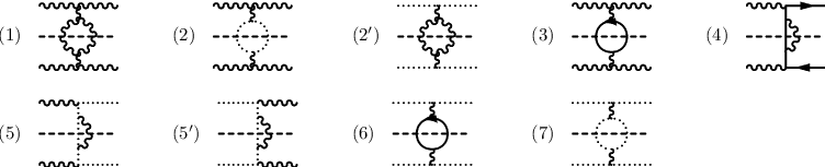
Refer to caption
Figure 23: Box graphs that contribute to the integral equation for V^g\hat{V}_{g}.
Refer to caption
Figure 24: Bubble graphs that contribute to the integral equation for V^g\hat{V}_{g}.
Refer to caption
Figure 25: Triangle graphs that contribute to the integral equation for V^g\hat{V}_{g}.
Refer to caption
Figure 26: Crossed-box graphs that contribute to the integral equation for V^g\hat{V}_{g}.
Refer to caption
Figure 27: Loly, tent and fish graphs that contribute to the integral equation for V^g\hat{V}_{g}.

(2) We calculate the Keldysh structure for each diagram. In order to do this, we look at the corresponding diagram where all lines are scalars, in the sense that they have no Dirac or Lorentz structure, but carry the appropriate boson or fermion thermal distribution functions. The summations over Keldysh indices are done using a Mathematica program. The program is described in [34] and is available at www.brandonu.ca/physics/fugleberg/Research/Dick.html. The program can be used to calculate the integrand corresponding to any diagram (up to five external legs) in the Keldysh, RA or 1-2 basis. The user supplies input in the form of lists of momenta and vertices for each propagator and vertex. Several examples of this part of the calculation are worked out in detail in [15]. We extract the overall phase space factor:

ℱ=∫l1∫l2:=1(2​π)3​ 2​El11(2​π)3​ 2​El2,\displaystyle{\cal F}=\int_{l_{1}}\int_{l_{2}}:=\frac{1}{(2\pi)^{3}\,2E_{l_{1}}}\,\frac{1}{(2\pi)^{3}\,2E_{l_{2}}}\,, (70)

and define the mandelstam variables:

s=(L1+L2)2;t=(P−L1)2;u=(P−L2)2.\displaystyle s=(L_{1}+L_{2})^{2}\,;~~t=(P-L_{1})^{2}\,;~~u=(P-L_{2})^{2}\,. (71)

The results are listed below. The notation ‘den’ is a reminder that the contributions from the numerators, produced by correctly including the appropriate Dirac and Lorentz structure, are not yet included.

den⁡[box⁡(1)]=ℱ​N​(bbbb)⋅1t2;i∈{1,5,6,7,9,10},\displaystyle{\rm den[box(1)]}={\cal F}\,{\rm N}({\rm bbbb})\cdot\frac{1}{t^{2}}\,;~~i\in\{1,5,6,7,9,10\}\,, (72)
den[box(2)]=ℱN(bbff)⋅1t2,den[box(3)]=den[box(4)]=den[box(8)]=−ℱN(bfbf)⋅1t2,\displaystyle{\rm den[box(2)]}={\cal F}\,{\rm N}({\rm bbff})\cdot\frac{1}{t^{2}}\,,~~{\rm den[box(3)]}={\rm den[box(4)]}={\rm den[box(8)]}=-\,{\cal F}\,{\rm N}({\rm bfbf})\cdot\frac{1}{t^{2}}\,,
den⁡[bub⁡(1)]=ℱ​N​(bbbb)⋅1s2;i∈{1,2,5,7},\displaystyle{\rm den[bub(1)]}={\cal F}\,{\rm N}({\rm bbbb})\cdot\frac{1}{s^{2}}\,;~~i\in\{1,2,5,7\}\,,
den[bub(3)]=den[bub(6)]=ℱN(bbff)⋅1s2,den[bub(4)]=−ℱN(bfbf)⋅1s2,\displaystyle{\rm den[bub(3)]}={\rm den[bub(6)]}={\cal F}\,{\rm N}({\rm bbff})\cdot\frac{1}{s^{2}}\,,~~{\rm den[bub(4)]}=-\,{\cal F}\,{\rm N}({\rm bfbf})\cdot\frac{1}{s^{2}}\,,
den⁡[tri⁡(1)]=ℱ​N​(bbbb)⋅1s​t;i∈{1,3,6,7,8,9},\displaystyle{\rm den[tri(1)]}={\cal F}\,{\rm N}({\rm bbbb})\cdot\frac{1}{st}\,;~~i\in\{1,3,6,7,8,9\}\,,
den[tri(2)]=ℱN(bbff)⋅1s​t,den[tri(4)]=−ℱN(bfbf)⋅1s​t,den[tri(5)]=−ℱN(bfbf)⋅1s​t,\displaystyle{\rm den[tri(2)]}={\cal F}\,{\rm N}({\rm bbff})\cdot\frac{1}{st}\,,~~{\rm den[tri(4)]}=-\,{\cal F}\,{\rm N}({\rm bfbf})\cdot\frac{1}{st}\,,~~{\rm den[tri(5)]}=-\,{\cal F}\,{\rm N}({\rm bfbf})\cdot\frac{1}{st}\,,
den⁡[cross⁡(1)]=ℱ​N​(bbbb)⋅1t​u;i∈{1,3,5,6,7},\displaystyle{\rm den[cross(1)]}={\cal F}\,{\rm N}({\rm bbbb})\cdot\frac{1}{tu}\,;~~i\in\{1,3,5,6,7\}\,,
den[cross(2)]=ℱN(bbff)⋅1t​u,den[cross(4)]=−ℱN(bfbf)⋅1t​u,\displaystyle{\rm den[cross(2)]}={\cal F}\,{\rm N}({\rm bbff})\cdot\frac{1}{tu}\,,~~{\rm den[cross(4)]}=-\,{\cal F}\,{\rm N}({\rm bfbf})\cdot\frac{1}{tu}\,,
den⁡[loly]=ℱ​i​N​(bbbb)⋅1s,den⁡[tent]=ℱ​i​N​(bbbb)⋅1t,den⁡[fish]=−ℱ​N​(bbbb).\displaystyle{\rm den[loly]}={\cal F}\,i\,{\rm N}({\rm bbbb})\cdot\frac{1}{s}\,,~~{\rm den[tent]}={\cal F}\,i\,{\rm N}({\rm bbbb})\cdot\frac{1}{t}\,,~~{\rm den[fish]}=-{\cal F}\,{\rm N}({\rm bbbb})\,.

The results for the numerators are given in (73) and are listed in the same order as the diagrams in the corresponding figure. For example, the first line in (73) gives the numerators for the box graphs labeled (1), (2), etc. The crossed-box graphs produce two contributions each, because there is a horizontal and a vertical cut.

num[box]={8(69​t22−25su)CA2,−8tuCF2dF,−8stCF2dF, 4(4s2+3us+4u2)CACFdF,\displaystyle{\rm num}[{\rm box}]=\left\{\right.8\left(\frac{69t^{2}}{2}-25su\right)C_{A}^{2},\;-8tuC_{F}^{2}d_{F},\;-8stC_{F}^{2}d_{F},\;4\left(4s^{2}+3us+4u^{2}\right)C_{A}C_{F}d_{F}, (73)
−2(t2+10su)CA2, 2t2CA2, 2t2CA2,−16suCA3CFdF, 4(s24+u24)CA2, 2t2CA2},\displaystyle~~~~-2\left(t^{2}+10su\right)C_{A}^{2},\;2t^{2}C_{A}^{2},\;2t^{2}C_{A}^{2},\;-16suC_{A}^{3}C_{F}d_{F},\;4\left(\frac{s^{2}}{4}+\frac{u^{2}}{4}\right)C_{A}^{2},\;2t^{2}C_{A}^{2}\left.\right\}\,,
num[bub]={8(69​s22−25tu)CA2, 2(−s2−10tu)CA2, 4(4t2+3ut+4u2)CACFdF,−8stCF2dF,2s2CA2,\displaystyle{\rm num}[{\rm bub}]=\left\{\right.8\left(\frac{69s^{2}}{2}-25tu\right)C_{A}^{2},\;2\left(-s^{2}-10tu\right)C_{A}^{2},\;4\left(4t^{2}+3ut+4u^{2}\right)C_{A}C_{F}d_{F},\;-8stC_{F}^{2}d_{F},2s^{2}C_{A}^{2},
−2tuCACFdF, 4(t24+u24)CA2},\displaystyle~~~~-2tuC_{A}C_{F}d_{F},\;4\left(\frac{t^{2}}{4}+\frac{u^{2}}{4}\right)C_{A}^{2}\left.\right\}\,,
num⁡[tri]={8​(15​s​u−3​t24)​CA2, 4​u2​CA​CF​dF,u2​CA2,0, 4​s2​CA​CF​dF, 0,−s2​CA2,t2​CA2,−u2​CA2},\displaystyle{\rm num}[{\rm tri}]=\left\{8\left(15su-\frac{3t^{2}}{4}\right)C_{A}^{2},\;4u^{2}C_{A}C_{F}d_{F},\;u^{2}C_{A}^{2},0,\;4s^{2}C_{A}C_{F}d_{F},\,0,\;-s^{2}C_{A}^{2},\;t^{2}C_{A}^{2},\;-u^{2}C_{A}^{2}\right\}\,,
num⁡[cross−horz]={4​(30​t​u−3​s22)​CA2, 0, 0, 4​u2​CA​CF​dF,−u2​CA2,u2​CA2, 0},\displaystyle{\rm num}[{\rm cross-horz}]=\left\{4\left(30tu-\frac{3s^{2}}{2}\right)C_{A}^{2},\;0,\;0,\;4u^{2}C_{A}C_{F}d_{F},\;-u^{2}C_{A}^{2},\;u^{2}C_{A}^{2},\;0\right\}\,,
num⁡[cross−vert]={4​(30​t​u−3​s22)​CA2,0,0, 4​u2​CA​CF​dF,−u2​CA2,t2​CA2,s2​CA2},\displaystyle{\rm num}[{\rm cross-vert}]=\left\{4\left(30tu-\frac{3s^{2}}{2}\right)C_{A}^{2},0,0,\;4u^{2}C_{A}C_{F}d_{F},\;-u^{2}C_{A}^{2},\;t^{2}C_{A}^{2},\;s^{2}C_{A}^{2}\right\}\,,
num⁡[loly/tent/fish]={324,i​CA2​s,324​i​CA2​s,−864​CA2}.\displaystyle{\rm num}[{\rm loly/tent/fish}]=\left\{324,i\,C_{A}^{2}\,s,324\,i\,C_{A}^{2}\,s,-864\,C_{A}^{2}\right\}\,.

The last step is to sum all contributions and show that:

∑(i)factor⁡[i]​num​[i]​den​[i]=ℱ⁡(ℳg​g→g​g​N​(bbbb)+ℳg​g→q​q¯​N​(bbff)+ℳg​q→g​q​N​(bfbf)+ℳg​q¯→g​q¯​N​(bfbf)).\displaystyle\sum_{(i)}{\rm factor}[i]{\rm num}[i]{\rm den}[i]={\cal F}\big({\rm{\cal M}}^{gg\to gg}\,{\rm N}({\rm bbbb})+{\rm{\cal M}}^{gg\to q\bar{q}}\,{\rm N}({\rm bbff})+{\rm{\cal M}}^{gq\to gq}\,{\rm N}({\rm bfbf})+{\rm{\cal M}}^{g\bar{q}\to g\bar{q}}\,{\rm N}({\rm bfbf})\big)\,. (74)

The sum over (i)(i) is over all of the graphs in Figs. 23, 24, 25, 26 and 27. We use the fact that the definitions of the internal momenta L1L_{1} and L2L_{2} can always be reversed, or equivalently, that each term can be written in a symmetric form by interchanging tt and uu. Note that when we insert the result for |ℳa​b→c​d|2\big|{\bf{\cal M}}^{ab\rightarrow cd}\big|^{2} into Eqn. (54), we must introduce an extra factor 1/2 if the final states cc and dd are not the same, to avoid double counting this contribution. These factors of two are indicated in square brackets in (75). The results are:

|ℳg​g→g​g|2=16​dA​CA2​(3−s​tu2−s​ut2−t​us2),\displaystyle\big|{\bf{\cal M}}^{gg\rightarrow gg}\big|^{2}=16\,d_{A}\,C_{A}^{2}\,\bigg(3-\frac{st}{u^{2}}-\frac{su}{t^{2}}-\frac{tu}{s^{2}}\bigg)\,, (75)
|ℳg​g→q​q¯|2=[12]​ 16​dF​CF​(CF​(tu+ut)−CA​(t2s2+u2s2)),\displaystyle\big|{\bf{\cal M}}^{gg\rightarrow q\bar{q}}\big|^{2}=\big[\frac{1}{2}\big]\,16\,d_{F}\,C_{F}\,\bigg(C_{F}\,\bigg(\frac{t}{u}+\frac{u}{t}\bigg)-C_{A}\,\bigg(\frac{t^{2}}{s^{2}}+\frac{u^{2}}{s^{2}}\bigg)\bigg)\,,
|ℳg​q→g​q|2=|ℳg​q¯→g​q¯|2=[12]​ 16​dF​CF​(CA​(s2t2+u2t2)−CF​(su+us)),\displaystyle\big|{\bf{\cal M}}^{gq\rightarrow gq}\big|^{2}=\big|{\bf{\cal M}}^{g\bar{q}\rightarrow g\bar{q}}\big|^{2}=\big[\frac{1}{2}\big]\,16\,d_{F}\,C_{F}\,\bigg(C_{A}\,\bigg(\frac{s^{2}}{t^{2}}+\frac{u^{2}}{t^{2}}\bigg)-C_{F}\,\bigg(\frac{s}{u}+\frac{u}{s}\bigg)\bigg)\,,

in agreement with (57).

References

  • [1] G. Aarts, PoSLAT2007, 001 (2007) - arXiv:0811.1850.
  • [2] P. Arnold, G. Moore and L.G. Yaffe, JHEP 0011, 001 (2000) - arXiv:hep-ph/0010177.
  • [3] P. Arnold, G.D. Moore and L.G. Yaffe, JHEP 0301, 030 (2003) - arXiv:hep-ph/0209353.
  • [4] P. Arnold, G.D. Moore and L.G. Yaffe, JHEP 0305, 051(2003) - arXiv:hep-ph/0302165.
  • [5] S. Jeon, Phys. Rev. D52, 3591 (1995) - arXiv:hep-ph/9409250.
  • [6] S. Jeon and L.G. Yaffe, Phys. Rev. D53, 5799 (1996) - arXiv:hep-ph/9512263.
  • [7] M.E. Carrington, D. Hou and R. Kobes, Phys. Rev. D62, 025010 (2000) - arXiv:hep-ph/9910344.
  • [8] E. Wang and U. Heniz, Phys. Rev. D67, 025022 (2003) - arXiv:hep-ph/02001116.
  • [9] M.A. Valle Basagoiti, Phys. Rev. D66, 045005 (2002) - arXiv:hep-ph/0204334.
  • [10] G. Aarts and J.M. Martinez-Resco, JHEP 0211, 022 (2002) - arXiv:hep-ph/0209048.
  • [11] D. Boyanovsky, H.J. deVega and S.Y. Wang, Phys. Rev. D67, 065022 (2003) - arXiv:hep-ph/0212107.
  • [12] J.-S. Gagnon and S. Jeon, Phys. Rev. D75, 025014 (2007) - arXiv:hep-ph/0610235.
  • [13] J.-S. Gagnon and S. Jeon, Phys. Rev. D75, 025014 (2007) - arXiv:hep-ph/0610235.
  • [14] G. Aarts and J.M. Martinez-Resco, JHEP 0503, 074 (2005) - arXiv:hep-ph/0503161.
  • [15] M.E. Carrington and E. Kovalchuk, Phys. Rev. D76, 045019 (2007) - arXiv:0705.0162.
  • [16] M.E. Carrington and E. Kovalchuk, Phys. Rev. D77, 025015 (2008) - arXiv:0709.0706.
  • [17] Hou Defu - arXiv:hep-ph/0501284.
  • [18] J. Berges, Phys. Rev. D70, 105010 (2004) - arXiv:hep-ph/0401172.
  • [19] A. Arrizabalaga and J. Smit, Phys. Rev. D66, 065014 (2002) - arXiv:hep-ph/0301093.
  • [20] M.E. Carrington, G. Kunstatter and H. Zaraket, Eur. Phys. J. C42, 253 (2005) - arXiv:hep-ph/0309084.
  • [21] G. Baym and L. Kadanoff, Phys. Rev. 124, 287 (1961).
  • [22] H. van Hees and J. Knoll, Phys. Rev. D66, 025028 (2002) - arXiv:hep-ph/0203008.
  • [23] J. Berges, S. Borsanyi, U. Reinosa and J. Serreau, Annals Phys. 320, 344 (2005) - arXiv:hep-ph/0503240.
  • [24] U. Reinosa and J. Serreau, JHEP 0607, 028 (2006) - arXiv:hep-th/0605023.
  • [25] U. Reinosa and J. Serreau, JHEP, 0711, 097 (2007) - arXiv:0708.0971.
  • [26] J. Berges, AIP Conf. Proc. 739, 3 (2005) - arXiv:hep-ph/0409233.
  • [27] J.M. Cornwall, R. Jackiw and E. Tomboulis, Phys. Rev. D10, 2428 (1974).
  • [28] M.E. Carrington, Hou Defu and R. Kobes, Phys. Rev. D67, 025021 (2003) - arXiv:hep-ph/0207115.
  • [29] N.P. Landsman and Ch. G. van Weert, Phys. Rep. 145, 141 (1987).
  • [30] B.L. Combridge, J. Kripfgamz and J. Ranft, Phys. Rev. Lett B70, 234 (1977).
  • [31] P.C. Martin and J. Schwinger, Phys. Rev. 115, 1432 (1959).
  • [32] L.V. Keldysh, Sov. Phys. JETP 20, 1018 (1965).
  • [33] F. Gelis, Nucl. Phys. B508, 483 (1997) - arXiv:hep-ph/9701410.
  • [34] M.E. Carrington, T. Fugleberg, D.S. Irvine and D. Pickering; Eur.Phys.J. C50, 711 (2007) - arXiv:hep-ph/0608298.
  • [35] C.D. Palmer and M.E. Carrington, Can. J. Phys. 80, 847 (2002) - arXiv:hep-th/0108088.