Thermoelectric spin transfer in textured magnets

The notion of the Berry phase[1] naturally appears in the description of magnetic texture dynamics in the limit of strong exchange field.[2, 3] The spin up and down with respect to local magnetization electrons experience “fictitious” electromagnetic fields.[4] These fields have opposite signs for spin up and down electrons and result in the Lorentz force.[2] It has been realized that the spin-transfer torque (STT) is a reciprocal effect to the electromotive force (EMF) associated with this Lorentz force.[5] In real systems, the exchange field is finite leading to spin misalignments with the texture, and more realistic description should take such effects into account via $\beta$ terms in the Landau-Lifshitz-Gilbert (LLG) equation.[6, 7]

Recently, interest in thermoelectric effects has considerably increased as new experimental data has been available.[8] The Peltier effect describes heat transfer accompanying the current flow. The opposite is the Seebeck effect that describes the thermo-EMF induced by temperature gradients. The Peltier and Seebeck thermoelectric effects as well as the thermoelectric STTs have been studied in multilayered nanostructures.[9] Hatami et al. proposed a thermoelectric STT as mechanism for domain wall motion.[9] Berger and Jen and Berger observed and discussed domain wall (DW) motion induced by heat currents.[10] Thermal STTs may soon be employed in the next generation of nonvolatile data elements for reversal of magnetization. Thermoelectric nano-coolers can find applications in the nanoelectronic circuits and devices.[11]

In this Rapid Communication, we study continuous magnetic systems which can be relevant to DW motion[12] and spin-textured magnets.[13] We phenomenologically describe thermal STTs in a quasi-1D magnetic wire with magnetic texture. The Berry-phase gauge field induced energy flow turns out to be reciprocal effect to the thermal STT and both effects can be formally eliminated from the equations of motion by properly redefining the thermodynamic variables which is reminiscent of the non-dissipative STTs.[5] We further generalize our description by including viscous $\beta-$like terms corresponding to spin misalignments. These viscous effects turn out to be important for the thermally induced DW motion and can lead to such effects as cooling by magnetic texture dynamics. We also find that the Peltier and Seebeck effects can be modified and tuned by the magnetic texture dynamics.

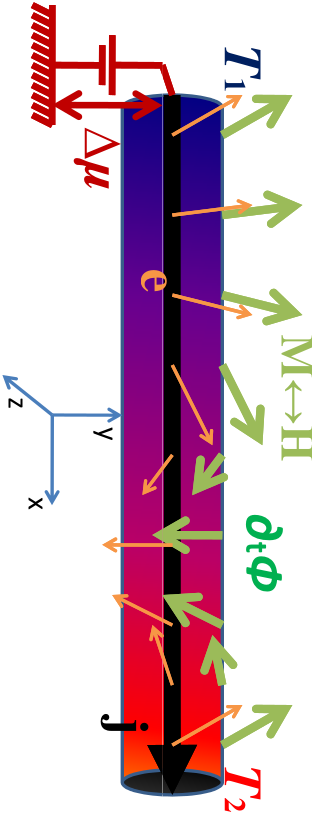
Consider a thin quasi-1D magnetic wire with the magnetization $\mathbf{m}(x,t)$ (along the spin density) in the presence of chemical potential $\mu(x,t)$ and temperature $T(x,t)$ gradients. We would like to construct a phenomenological description of our system based on thermodynamic variables introduced above and their conjugate forces. The ferromagnetic wire is supposed to be thermally isolated, and after being perturbed by nonequilibrium chemical potential, magnetization and temperature gradients, the wire evolves back toward equilibrium according to the equations of motion, producing entropy. Note that we allow this equilibrium state to be topologically nontrivial, e.g. a magnetic DW or vortex. The state of partial equilibrium can be described by thermodynamic variables $x_{i}$ and their conjugates (generalized forces) $X_{i}=\partial\mathbb{S}/\partial x_{i}$ with the entropy and its time derivative being:

We initially consider the entropy $\mathbb{S}(\rho,\rho_{U},\mathbf{m})$ as a function of the density of electron charge $\rho$, the density of energy $\rho_{U}$ and the magnetization direction. The magnitude of the magnetization is not treated as a dynamic variable, assuming sufficiently fast spin-flip relaxation. The conservation laws of energy and charge provide linear relations:

where we introduced the charge current $j$ and energy current $j_{U}$. For conserved quantities, it is more convenient to work with fluxes $j$ and $j_{U}$ instead of densities $\rho$ and $\rho_{U}$ which leads to equivalent description due to the linear relations in Eqs. (1).

We will not be concerned with the general expression for the entropy but rather concentrate on identifying the thermodynamic variables and their conjugates by calculating the time derivative of the entropy. Suppose that we fix the texture, then the rate of the entropy change is:[14]

where we introduced the modified energy current $j_{q}=j_{U}-\mu j$ that describes the energy flow without the energy corresponding to the chemical potential $\mu$ (from now on only the energy current $j_{q}$ is considered). The chemical potential is defined as a conjugate of the density of charge. The introduction of $j_{q}$ is necessary to avoid the unphysical gauge dependence of the energy current and the associated kinetic coefficients on the potential offset for the whole system. We are now ready to write the rate of the entropy change for the general case of dynamic spin texture:

where in Eq. (2) we integrated the term involving $j_{q}$ by parts and the conjugate/force corresponding to the magnetization is defined as $-\partial_{\mathbf{m}}\mathbb{S}|_{Q,q}=\mathbf{H}/T$ with $Q(x)$ and $q(x)$ being the overall charge and energy that passed the cross section at point $x$ which corresponds to integrating $j$ and $j_{q}$ in time, respectively. As it can be seen from Eq. (3), our other conjugates are $-\partial_{q}\mathbb{S}|_{\mathbf{m},Q}=-\partial_{x}\left(1/T\right)$ and $-\partial_{Q}\mathbb{S}|_{\mathbf{m},q}=\partial_{x}\mu/T$. In general, $\mathbf{H}$ is not the usual “effective field” corresponding to the variation of the Landau free-energy functional $F[\mathbf{m},\mu,T]$ and only when $\partial_{x}T=0$ and $\partial_{x}\mu=0$ the “effective fields” coincide. Let us initially assume that even in an out-of-equilibrium situation, when $\partial_{x}T\neq 0$ and $\partial_{x}\mu\neq 0$, $\mathbf{H}$ depends only on the instantaneous texture $\mathbf{m}(x)$. In general, however, we may expand $\mathbf{H}$ phenomenologically in terms of small $\partial_{x}T$ and $\partial_{x}\mu$.

In our phenomenological theory, the time derivatives of thermodynamic variables are related to the thermodynamic conjugates via the kinetic coefficients. In order to identify the kinetic coefficients, we assume that the currents $j$ and $j_{q}$ are determined by the chemical potential and temperature gradients as well as the magnetic wire dynamics, which exerts fictitious Berry phase gauge fields[5] on the charge transport along the wire. We then have for the charge/energy current gradient expansion:

where we assume that the coefficients $\tilde{g}$, $\tilde{\xi}$ and $\tilde{\zeta}$ can in general also depend on temperature and texture, for the latter, to the leading order, as $\tilde{g}=\tilde{g}_{0}+\eta_{\tilde{g}}(\partial_{x}\mathbf{m})^{2}$, etc.. In Eqs. (4) and (5), we expand only up to the linear order in the nonequilibrium quantities $\partial_{x}\mu$, $\partial_{x}T$ and $\partial_{t}\mathbf{m}$ and to the second order in $\partial_{x}\mathbf{m}$; however, the latter terms are expected to be small in practice and only are necessary for establishing the positive-definiteness of the response matrix. The spin-rotational symmetry of the magnetic texture and the inversion symmetry of the wire are also assumed to avoid additional and often complicated terms in our expressions. Relating $\partial_{t}\mathbf{m}$ to the generalized force $-\mathbf{H}/T$, within the LLG[15] phenomenology, we derive the modified LLG equation consistent with Eqs. (4) and (5), with the guidance of the Onsager reciprocity principle:

where we introduced the spin density $s$ so that $s\mathbf{m}=\mathbf{M}/\gamma$, with $M$ being the magnetization density and $\gamma$ the gyromagnetic ratio ($\gamma<0$ for electrons). Equation (6) can be expressed in terms of the charge/energy flows by inverting the linear relation $\{j,j_{q}\}=\{\tilde{g},\tilde{\xi};\tilde{\xi},\tilde{\kappa}\}\{\partial_{x}\mu,\partial_{x}T/T\}$:

where the new coefficients $g$, $\xi$, $\zeta$, $p$, $p^{\prime}$, $\beta$ and $\beta^{\prime}$ can be expressed via the ones marked by tilde, and in Eq. (9), we disregarded the terms of the order $\sim(\partial_{x}\mathbf{m})^{2}\partial_{t}\mathbf{m}$ contributing to the Gilbert damping. Terms of similar order can also appear in case of incompressible charge flow and lead to the non-local Gilbert damping.[5] The kinetic coefficients contain information about the conductivity, $\sigma=\tilde{g}$, the thermal conductivity, $\kappa=1/(\zeta T)$, and the conventional Seebeck and Peltier coefficients can be found from Eqs. (4) and (8) by assuming $j=0$ for the former, $S=-\tilde{\xi}/(\tilde{g}T)$, and by assuming $\partial_{x}T=0$ for the latter, $\Pi=\xi/\zeta=-\tilde{\xi}/\tilde{g}$, which also implies that $g=1/\sigma+S^{2}T/\kappa$. Equation (9) differs from an ordinary LLG equation[7] by the extra spin torque terms that appear in the presence of the energy flow $j_{q}$. These new torques are similar to the nondissipative and dissipative current induced spin torques,[5] as the former can be related to electron spins following the magnetic texture and the latter - to electron spins mistracking the texture. The phenomenological parameter $\tilde{p}$ (or $p=\tilde{p}/\sigma_{0}-p^{\prime}\Pi_{0}$) can be approximated as $\tilde{p}/\sigma_{0}=\wp\hbar/2e$ in the strong exchange limit[5] and corresponds to the electron spin-charge conversion factor $\hbar/2e$ multiplied by the polarization $\wp=(\sigma_{0}^{\uparrow}-\sigma_{0}^{\downarrow})/\sigma_{0}$, $\sigma_{0}=\sigma_{0}^{\uparrow}+\sigma_{0}^{\downarrow}$ and $e$ is minus the charge of particles, e.g. for electrons $e$ is positive.

Similarly, we can consider Eq. (9) under conditions of vanishing charge currents and fixed texture, and find the spin current resulting from the temperature gradients: $2eS_{s}\partial_{x}T/(1/\sigma_{0}^{\uparrow}+1/\sigma_{0}^{\downarrow})$ where $S_{s}=(S_{0}^{\uparrow}-S_{0}^{\downarrow})/e$ is the spin Seebeck coefficient in the absence of magnetic texture. By involving the electron spin-charge conversion factor again, we can approximate the second spin torque parameter $p^{\prime}$ in Eq. (9) in the strong exchange limit arriving at

where we introduced the spin polarization of the Seebeck coefficient $\wp_{S}=(S_{0}^{\uparrow}-S_{0}^{\downarrow})/(S_{0}^{\uparrow}+S_{0}^{\downarrow})=eS_{s}/(2S_{0})$. When the thermal conductivity is mostly due to electron motion, we can simplify Eq. (10) further with the help of the Wiedemann-Franz Law according to which $\kappa_{0}/\sigma_{0}=LT$ where $L=\pi^{2}k_{B}^{2}/(3e^{2})$ is the Lorenz number. Effects such as spin drag[16] can also influence the estimate in Eq. (10). Note that the result in Eq. (10) can also be obtained from Eq. (8) by considering the texture-dynamics induced EMF which can lead to the energy currents in the absence of charge currents.

One can redefine the magnetization (which in turn leads to changes in generalized forces $\partial_{x}\mu/T$ and $\partial_{x}T/T^{2}$) in Eq. (3) so that the nondissipative parts of torques are absorbed into these new definitions:

where with this choice of thermodynamic variables, Eqs. (7), (8) and (9) will only have spin torque terms proportional to $\beta(\beta^{\prime})$.

From Eq. (3), we can write the rate of the entropy production:

where $g=g_{0}+\eta_{g}(\partial_{x}\mathbf{m})^{2}$, $\xi=\xi_{0}+\eta_{\xi}(\partial_{x}\mathbf{m})^{2}$ and $\zeta=\zeta_{0}+\eta_{\zeta}(\partial_{x}\mathbf{m})^{2}$. Notice that the STTs in Eq. (9) induced by the charge/energy currents can be separated into the nondissipative and dissipative parts ($\beta$ terms) based on Eq. (11). This separation is, nevertheless, formal as in realistic metallic systems the torques will always be accompanied by the dissipation due to the finite thermal conductivity $\kappa$ and conductivity $\sigma$. The dissipation in Eq. (11) is guaranteed to be positive-definite if the following formal inequalities hold:

where the first inequality can be rewritten equivalently as $g\geq S^{2}T/\kappa$, and should always hold. Other inequalities are somewhat formal since their proof implies that our theory can describe sufficiently sharp and fast texture dynamics for dominating dissipation as opposed to the first inequality for proof of which a mere static texture assumption is sufficient. Nevertheless, Eqs. (12) can serve for estimates of the spin-texture resistivities ($\eta_{\zeta}$ and $\eta_{g}$) and the spin-texture Seebeck effect ($\eta_{\xi}$) due to spin dephasing. The condition on the spin-texture resistivity[5] $\eta_{1/\sigma}\geq(\tilde{\beta}\tilde{p})^{2}/(\alpha s\sigma_{0}^{2})$ also follows from Eqs. (12).

Let us now discuss thermal effects that can arise from the presence of magnetic texture. In case of a static spin texture and stationary charge density, $\partial_{x}j=0$, we can write the modification to the Thomson effect by calculating the rate of heat generation[14] $\dot{\mathbb{Q}}=-\partial_{x}j_{U}$ from Eqs. (4) and (8):

where $\kappa=\kappa_{0}+\eta_{\kappa}(\partial_{x}\mathbf{m})^{2}$ and $S=S_{0}+\eta_{S}(\partial_{x}\mathbf{m})^{2}$. Even though Eqs. (4) and (8) are the first order gradient expansions, they are sufficient for obtaining Eq. (13) since consideration of the second order expansions would only lead to even higher order terms in Eq. (13). The Thomson effect can be modified by the presence of texture and some analogue of local cooling may be possible even without temperature gradients. However, the magnitude of the coefficients $\eta_{\kappa}$ and $\eta_{S}$ is not accessible at the moment and should be extracted from the microscopic calculations.

Another thermal effect we would like to discuss is related to heat flows induced by magnetization dynamics. As can be seen from Eq. (8), such heat flows can appear even in the absence of temperature gradients and charge current flows. When the magnetic texture follows a periodic motion, the energy flows should result in effective cooling or heating of some regions by specifically engineering the magnetic state of the wire and applied rf magnetic fields. The spin spring magnets can be of relevance.[17] Alternatively, the texture in our wire (i.e. spiral), can result from the Dzyaloshinskii-Moriya (DM) interaction[14] relevant for such materials as MnSi, (Fe,Co)Si or FeGe. In this case, the end of the spiral can be exchange coupled to a homogeneous magnetization of a magnetic film subject to rf magnetic field which should result in rotation of the magnetization in the film and spiral.

To simulate the spiral rotation and obtain the preliminary estimates of the effect, we consider the current induced spiral motion that in turn leads to the energy flows due to the magnetic texture dynamics. The static texture corrections due to $\eta-$ type terms will be ignored. We consider a ferromagnetic wire with the DM interaction in the absence of the temperature gradients. The “effective field” can be found from the Free energy:[14]

where $J$ is the exchange coupling constant and $\Gamma$ is the strength of the DM interaction. The “effective field” $\mathbf{H}\equiv\partial_{\mathbf{m}}F$ can be used in the LLG Eq. (9). The ground state of the Free energy in Eq. (14) is a spiral state $\mathbf{m}(\mathbf{r})=\mathbf{n}_{1}\cos\mathbf{k}\cdot\mathbf{r}+\mathbf{n}_{2}\sin\mathbf{k}\cdot\mathbf{r}$ where the wavevector $\mathbf{k}=\mathbf{n}_{3}\Gamma/J$, and $\mathbf{n}_{i}$ form the right handed orthonormal vector sets. We assume that the wavevector is along the wire, e.g. due to anisotropies. As can be found from the LLG Eq. (6), for the case of vanishing temperature gradients, the spiral starts to move along the wire in the presence of currents and the solution can be described as[18]

where the $x$ axis points along the wire axis, $m_{x}=(j\hbar/e)(\beta/\alpha-1)/(2\Gamma-Jk)$, $m_{\perp}=\sqrt{1-m_{x}^{2}}$ and $\upsilon=\wp j(\tilde{\beta}/\alpha)s\hbar/(2e)$. The wavenumber $k=2\pi/\lambda$ and $m_{x}$ have been calculated numerically in Ref. 18 and in the presence of currents $\lambda$ increases and $m_{x}$ acquires some finite value; however, for an estimate corresponding to moderate currents the values given by the static spiral $k_{0}=\Gamma/J$ should suffice. The maximum current that the spiral can sustain without breaking into the chaotic motion is $j_{max}\sim 2\Gamma e/\hbar$.[18]

Using Eq. (8), we are now ready to find the energy flow accompanying the current flow as the spiral moves with the speed $\upsilon$ in the absence of the temperature gradients: $j_{q}=\Pi_{0}j-m_{\perp}^{2}k^{2}\upsilon p^{\prime}\beta^{\prime}/\zeta\approx 0.8\Pi_{0}j$, where only $\beta^{\prime}-$ term contributes to the energy flow in Eq. (8). For our estimate, we take parameters corresponding to a MnSi:[13] the lattice constant $a=0.5$ nm, the magnetization density $M=0.4\mu_{B}/a^{3}$, $\lambda=20$ nm, $\alpha=0.01$, $\tilde{\beta}=\beta^{\prime}=0.03$, $\sigma=5\times 10^{7}\;\Omega^{-1}\mbox{m}^{-1}$, $Ja=0.02\;\mbox{eV}$ and $\wp=\wp_{S}=0.8$. By increasing $\tilde{\beta}(\beta^{\prime})$ and $\sigma$ and diminishing $\lambda$ and $\alpha$, the energy flow can be made larger. We conclude then that the current-induced magnetic texture dynamics can lead to additional energy flows that in some cases can be comparable to the energy flows due to the Peltier effect. The renormalization of the Peltier coefficient should also apply to the Seebeck coefficient due to the Onsager reciprocity principle dictating that $S=\Pi/T$. Assuming the absence of the temperature gradient, from Eq. (4), we also find correction to the conductivity caused by the EMF due to the spiral motion: $-\partial_{x}\mu=j/\sigma_{0}+m_{\perp}^{2}k^{2}\upsilon\wp\tilde{\beta}\hbar/(2e)\approx 0.8j/\sigma_{0}$.

Finally, we calculate the speed of the spiral motion induced by temperature gradients in the absence of charge currents. In full analogy to the spiral motion induced by the charge currents and using Eq. (9), we find the spiral speed induced by the temperature gradients:

Continuing this analogy between the energy currents and charge currents, we can generalize the applicability of the result in Eq. (15) to transverse Neel DW[7] under the assumption of constant temperature gradients and vanishing charge currents. Just like the $\beta$ term is important for the current-driven DW dynamics,[7] the new viscous $\beta^{\prime}$ term is important for the thermally induced DW motion below the Walker breakdown.

To conclude, we phenomenologically introduced new $\mbox{$\beta$}-$like viscous term into the LLG equation for the energy currents. We speculate on a possibility of creating heat flows by microwave-induced periodic magnetization dynamics which should result in effective cooling of some regions, in analogy to the Peltier effect. To support it, we considered the DM spiral texture subject to charge current and found that the texture-dynamics induced heat flow is proportional to the Peltier coefficient and the new viscous coupling constant $\beta^{\prime}$. Thus, the materials with large Peltier coefficient and large $\beta^{\prime}$ should be suitable for the realization of the microwave cooling by magnetization texture dynamics. The effective Peltier/Seebeck coefficient as well as the conductivity can be modified and tuned by the texture dynamics. These effects should be measurable in magnetic textures characterized by the length as small as $\sim 10$ nm and large viscous damping $\beta$. Even in situations of pinned textures, the effects of EMF induced by viscous $\beta-$like term should be seen in measurements of the ac conductivity. We also conclude that the new viscous $\beta^{\prime}$ term is important for the thermally induced DW motion. Bauer et al.[19] worked out very similar ideas for cooling by DW motion and thermoelectric excitation of magnetization dynamics.

We acknowledge the stimulating discussions with G. E. W. Bauer, A. Brataas and C. H. Wong. This work was supported in part by the Alfred P. Sloan Foundation.

References

- [1] M. V. Berry, Proc. R. Soc. London, Ser. A 392, 45 (1984).
- [2] S. E. Barnes and S. Maekawa, Phys. Rev. Lett. 98, 246601 (2007).
- [3] Y. Tserkovnyak and M. Mecklenburg, Phys. Rev. B 77, 134407 (2008).
- [4] G. E. Volovik, J. Phys. C 20, L83 (1987).
- [5] Y. Tserkovnyak and C. H. Wong, Phys. Rev. B 79, 014402 (2009).
- [6] S. Zhang and Z. Li, Phys. Rev. Lett. 93, 127204 (2004); A. Thiaville, Y. Nakatani, J. Miltat, and Y. Suzuki, Europhys. Lett. 69, 990 (2005); H. Kohno, G. Tatara, and J. Shibata, J. Phys. Soc. Jpn. 75, 113706 (2006); R. A. Duine, A. S. Nunez, J. Sinova, and A. H. MacDonald, Phys. Rev. B 75, 214420 (2007).
- [7] Y. Tserkovnyak, A. Brataas, and G. E. Bauer, J. Magn. Magn. Mater. 320, 1282 (2008).
- [8] B. C. Sales, Science 295, 1248 (2002); A. I. Hochbaum, R. Chen, R. D. Delgado, W. Liang, E. C. Garnett, M. Najarian, A. Majumdar, and P. Yang, Nature 451, 163 (2008), A. I. Boukai, Y. Bunimovich, J. Tahir-Kheli, J.-K. Yu, W. A. Goddard, and J. R. Heath, ibid. 451, 168 (2008).
- [9] M. Hatami, G. E. W. Bauer, Q. Zhang, and P. J. Kelly, Phys. Rev. B 79, 174426 (2009); M. Hatami, G. E. W. Bauer, Q. Zhang, and P. J. Kelly, Phys. Rev. Lett. 99, 066603 (2007).
- [10] L. Berger, J. Appl. Phys. 58, 450 (1985), S. U. Jen and L. Berger, ibid. 59, 1278 (1986a), S. U. Jen and L. Berger, ibid. 59, 1285 (1986b).
- [11] H. Ohta, S. Kim, Y. Mune, T. Mizoguchi, K. Nomura, S. Ohta, T. Nomura, Y. Nakanishi, Y. Ikuhara, M. Hirano, et al., Nature Mater. 6, 129 (2007).
- [12] A. Yamaguchi, T. Ono, S. Nasu, K. Miyake, K. Mibu, and T. Shinjo, Phys. Rev. Lett. 92, 077205 (2004), M. Hayashi, L. Thomas, Y. B. Bazaliy, C. Rettner, R. Moriya, X. Jiang, and S. S. P. Parkin, ibid. 96, 197207 (2006); M. Hayashi, L. Thomas, C. Rettner, R. Moriya, and S. S. P. Parkin, Nat. Phys. 3, 21 (2007).
- [13] S. Muhlbauer, B. Binz, F. Jonietz, C. Pfleiderer, A. Rosch, A. Neubauer, R. Georgii, and P. Boni, Science 323, 915 (2009).
- [14] L. Landau and E. Lifshitz, Electrodynamics of Continuous Media, vol. 8 (Pergamon, Oxford, 1984), 2nd ed.
- [15] T. Gilbert, IEEE Trans. Magn. 40, 3443 (2004).
- [16] I. D’amico and G. Vignale, Phys. Rev. B 62, 4853 (2000).
- [17] V. M. Uzdin and A. Vega, Nanotechnology 19, 315401 (2008).
- [18] K. Goto, H. Katsura, and N. Nagaosa, arXiv:0807.2901 (unpublished).
- [19] G. E. W. Bauer et al., preprint (unpublished).