ULB-TH/09-18
Sachs-Wolfe at second order:
the CMB bispectrum on large
angular scales
Lotfi Boubekeura,b,c, Paolo Creminellic, Guido D’Amicod,e,
Jorge Noreñad, and Filippo Vernizzif
a Departament de Física Teòrica and IFIC,
Universitat de València-CSIC, E-46100, Burjassot, Spain.
b Service de Physique Théorique, Université Libre de Bruxelles, 1050 Brussels, Belgium
c Abdus Salam International Centre for Theoretical Physics
Strada Costiera 11, 34014, Trieste, Italy
d SISSA, via Beirut 2-4, 34014, Trieste, Italy
e INFN - Sezione di Trieste, 34014 Trieste, Italy
f CEA, IPhT, 91191 Gif-sur-Yvette cédex, France
CNRS, URA-2306, 91191 Gif-sur-Yvette cédex, France
Abstract
We calculate the
Cosmic Microwave Background anisotropy
bispectrum on large angular scales
in the absence of primordial non-Gaussianities,
assuming exact matter dominance and extending
at second order the classic Sachs-Wolfe result . The calculation is done in Poisson gauge.
Besides intrinsic contributions calculated at last scattering, one must consider integrated effects. These are associated to
lensing, and to the time dependence of the potentials (Rees-Sciama) and of
the vector and tensor components of
the metric generated at second order.
The bispectrum is explicitly computed in
the
flat-sky
approximation.
It
scales as in
the scale invariant limit and
the shape dependence of its various
contributions is represented in 3d plots.
Although all the contributions to the bispectrum are parametrically of the same order, the full bispectrum is dominated by lensing. In the squeezed limit it corresponds to
, where is the
angle between the short and the long modes; the angle dependent
contribution comes from lensing. In the equilateral limit it
corresponds to .
1 Introduction
The linear approximation to cosmological perturbations has been so far sufficient and extremely fruitful, at least on large scales, before non-linearities induced by gravity become significant. However, the accuracy of observations is now reaching a level such that all second-order effects, naively of magnitude , may become relevant. This is particularly important in the context of primordial non-Gaussianities: second-order effects are in fact expected to give a signal of order few, which is not far from the present experimental limits [1, 2, 3]. A large amount of work has been done to study Cosmic Microwave Background (CMB) fluctuations beyond the linear approximation, in order to make predictions for the temperature bispectrum. As a complete calculation of the bispectrum is a daunting task, people concentrated on specific effects which are expected to dominate in particular limits. The bispectrum generated by the correlation between lensing and the Integrated Sachs-Wolfe (ISW) effect has been studied in [4, 5]. The one coming from lensing and the Sunyaev-Zel’dovich effect has been studied in [5]. In [6, 7, 8] the bispectrum generated by perturbations in the recombination history has been calculated. Refs [9, 10] (see also [11]) focused on very short angular scales where the signal is dominated by the non-linearity induced by dark matter clustering. A systematic control of all second-order effects in the Boltzmann equations is currently under study: see [12, 13] and references therein.
In this paper we calculate the CMB bispectrum in the limit of large angles, i.e. on angular scales larger than the one subtended by the Hubble radius at recombination (); we do this assuming perfect matter dominance. Important, although, as we will see, partial results were obtained in this regime in [14, 15, 16].
Our calculation can be seen as the extension to second order of the classic Sachs-Wolfe formula [17]
| (1.1) |
where is the Newtonian potential at recombination, which gives the large-angle prediction for the spectrum of the CMB fluctuations. As it is well known, this formula describes the angular variation of the temperature without considering the dynamics of the photon/baryon plasma, but only the gravitational redshift of photons from the last scattering to us. Therefore, it describes correctly the CMB anisotropies only in the limit where the scales considered are well out of the Hubble radius at recombination: the same restriction will apply to our calculation. The Sachs-Wolfe formula further assumes that decoupling took place when the universe was matter dominated – neglecting the transition between radiation and matter domination – and that the universe is still matter dominated nowadays, neglecting the present acceleration. At linear order this simplification is very convenient as the gravitational potential stays constant during matter dominance. At second-order the gravitational potential is no longer constant but the second-order metric during matter dominance is known [18] and can be written analytically as a function of the large-scale inflationary perturbations [16, 19].
Clearly, these approximations do not hold in the real universe. However, our calculations give the exact bispectrum in the same limit in which the Sachs-Wolfe formula becomes exact: zero cosmological constant, recombination that happens much after equality and in the limit in which all scales are much larger than the horizon at recombination. This last limit can be imagined by thinking about an experimentalist making measurements in the far future, when the angle subtended by the Hubble radius at recombination is minuscule. The fact that our results become exact in a well defined physical limit is quite important, as on large angular scales the separation among different effects is in general gauge dependent. Therefore, one has to be careful in making approximations because neglecting some effects leads, in general, to a gauge dependent result. Besides its theoretical interest, we expect our result to represent a fair approximation to the real universe on large angular scales and it can be taken as a starting point for more elaborated calculations.
Motivated by inflation, we assume that there are no vector or tensor perturbations in the initial conditions on super-Hubble scales. We perform the calculation of the CMB anisotropies by integrating the photon geodesic equation during matter dominance using the so called “generalized Poisson gauge”, which generalizes at second order the standard Newtonian gauge. Besides the Newtonian and curvature potential, at second order new terms are present in the metric, generated by the product of linear fluctuations: a vector mode in the entry of the metric, and a tensor mode in the spatial part.
All these terms contribute to the final CMB anisotropy. The time independent parts of the gravitational potentials give rise to second-order terms evaluated at last scattering, in analogy with eq. (1.1); their contribution was calculated in [14]. However, at second-order there are also terms integrated along the photon trajectory, similarly to what happens at first order when we depart from matter dominance with the ISW effect. The time-evolution at second order of the gravitational potential on sub-Hubble scales generates the well-known Rees-Sciama effect [20, 21]. But also the vector and tensor part of the metric contribute with two integrated terms.11 1 The integrated tensor contribution has been taken into account for the large scale anisotropies in [16]. The vector contribution has, to our knowledge, always been ignored. All these terms contain a number of spatial gradients higher than the intrinsic terms, so that one may think that they can be neglected on large scales as suppressed by positive powers of at recombination. However, this conclusion is too hasty: these terms are integrated along the photon trajectory while modes progressively reenter the Hubble radius. Thus the ratio should not be evaluated at recombination but when the terms contribute to the time integral. We will see that all the integrated pieces give a contribution of the same order as the intrinsic terms in the equilateral limit. Actually the separation between intrinsic and integrated effects has no physical, gauge invariant meaning. For example, a part of the integrated vector contribution will turn out to be a boundary term.
Another integrated contribution is gravitational lensing, due to the gravitational deflection of the photon trajectory with respect to the line of observation. Although the effect of lensing on the bispectrum through its correlation with the ISW effect is well known [4, 5] (but absent in our calculation as we are assuming perfect matter dominance), we will see that lensing is important also when correlated with intrinsic contributions at last scattering. In particular, we will find that lensing gives a squeezed limit contribution of the same order as the one due to intrinsic effects, but which depends on the angle between the long and the short modes. The effect of lensing on the bispectrum was studied in [22] with the conclusion that its effect is suppressed in the squeezed limit by the tilt of the spectrum. We will see that this conclusion is not correct.
In computing the CMB bispectrum we will employ the flat-sky approximation, which is valid for small angles of view. Given that at the same time we are interested in angles which are much larger than the Hubble radius at recombination, there is a quite narrow range of scales, , where our approximations hold. However, the flat-sky approximation greatly simplifies the algebra and makes the result much more transparent. The results will be given by 2-dimensional kernels , which can be thought of as the 2d observable analogue of the kernels used (in 3 dimensions) to describe the shape of the primordial non-Gaussianity [23].
The paper is organized as follows. In the next section we give the second-order metric in matter dominance in the generalized Poisson gauge as a function of the inflationary initial conditions and we calculate the temperature anisotropy at second order integrating the photon geodesic. In section 3 we make a general discussion about the bispectrum of the temperature anisotropy in the flat-sky approximation and we calculate this quantity induced by a primordial non-Gaussianity of the local and equilateral kind. These are useful for comparison with our results. In section 4 we calculate the bispectrum using the results of section 2. The calculation is split (for convenience, not because the effects are physically distinguishable) in various pieces: intrinsic effects at last scattering, integrated vector contribution, integrated tensor contribution and lensing. The resulting total bispectrum is discussed in section 5 and conclusions are drawn in section 6. The flat-sky approximation is discussed in appendix A, while the details of the calculation of the Rees-Sciama effect are presented in appendix B.
2 Second-order temperature anisotropies
In this section we calculate the CMB temperature anisotropy at second order in perturbations, in the large angular scale limit and for matter dominance, as a function of the angle of observation. On large angular scales, the effect of second-order perturbations on the CMB fluctuations have been studied more generally in [24, 25]. Although we will later use the flat-sky approximation, the results of this section hold also in a full-sky treatment.
We are interested in the CMB temperature fluctuations,
| (2.1) |
where is the observed photon temperature in the angular direction () and is its average over the sky. For a black-body spectrum the observed temperature is related to the one of emission by Liouville’s theorem: as phase space density is conserved in the propagation of photons (assuming there is no further scattering), the phase space density received in a given direction is the same as the one at emission but with a temperature [26, 17]
| (2.2) |
where and are the frequencies at emission and observation of a given photon. Notice that this statement is exact and therefore holds at any order in perturbation theory. In general, also the temperature at emission will not be isotropic, but will depend on the angle of emission. This dependence can be however neglected in our case, as we are interested in perturbations which are much longer than the horizon at recombination.
We work in the so called generalized Poisson gauge and use conformal time . In this gauge, the metric reads [18]
| (2.3) |
where is transverse, , and is transverse and traceless, . In the matter dominated era, assuming that the amount of primordial gravitational waves is negligible, the components of this metric are [18, 16, 19]
| (2.4) | ||||
| (2.5) | ||||
| (2.6) | ||||
| (2.7) |
The scalar quantities and are the Newtonian and curvature potentials, respectively, while we will refer to and as the vector and tensor components of the metric. The metric is expressed in terms of , the time-independent quantity representing the initial curvature perturbation generated during inflation. Indeed, is simply proportional to the (non-linear) curvature perturbation on uniform density hypersurfaces : on super-Hubble scales, where is constant,
| (2.8) |
In the following we are going to assume that on large scales, and therefore , is perfectly Gaussian, which is a very good approximation for example in minimal single field inflationary models [27, 28]. In the expression for tensor modes, the spherical Bessel function is given by , while is a transverse traceless projector defined as
| (2.9) |
where is a symmetric transverse projector given by
| (2.10) |
It can be expanded to give
| (2.11) |
with
| (2.12) |
In order to study the photon redshift we must solve the photon geodesic equation from last scattering to us, taking into account the perturbations of the metric above. The photon geodesic equation can be written as
| (2.13) |
where is the four-momentum of the photon, . The frequency of a photon with four-momentum as measured by an observer with four-velocity , is given by . For simplicity, we choose the observer today to have zero spatial velocity, . Indeed, any peculiar motion of the observer leads to a dipole anisotropy that can easily be subtracted. Furthermore, since we are interested in the large angular scales, we neglect also the Doppler effect due to the velocity of the photon/baryon fluid at recombination, which vanishes on super-Hubble scales at decoupling. Thus, we choose also the emitter to have zero spatial velocity, , so that we have both for the observer and the emitter. Making use of the normalization condition of the four-velocity, , one obtains , and thus
| (2.14) |
In order to compute we need to solve the time component of eq. (2.13). Using that and plugging the metric (2.3) into eq. (2.13) yields
| (2.15) |
where by a prime we denote the partial derivative with respect to conformal time, , and is the conformal Hubble rate, . One can immediately notice that the first term on the right hand side vanishes because of the massless condition . Note also that, as we are studying perfect matter dominance, the two potentials and are constant at linear order, see eqs. (2.4) and (2.5). Thus, their time derivatives , , together with and , are all second-order quantities. One can therefore replace the zeroth-order expression into this equation; furthermore, using the background relation , the geodesic equation can be finally rewritten as
| (2.16) |
that upon integration yields
| (2.17) |
Plugging this expression into eq. (2.14), one obtains the photon redshift up to second-order as a function of the metric perturbations,
| (2.18) |
Now we need to relate on the right hand side of eq. (2.2) to the metric perturbations at decoupling. Since we concentrate on large angular scales, we only need the super-Hubble relation. We will use adiabatic initial conditions. In this case the dark matter energy density simply scales as the third power of the temperature,
| (2.19) |
In the matter dominated era, the energy density of dark matter is related to the metric perturbations through the Einstein equations, in particular through the energy constraint equation. On super-Hubble scales, i.e. neglecting spatial gradients, and using the fact that the potentials and at first order are time-independent in the matter dominated era this reads, up to second order, (see for instance eq. (196) of [29])
| (2.20) |
where is the Hubble rate. Using the background Friedmann equation and eq. (2.19) above, this equation can be rewritten as
| (2.21) |
where is the average temperature at emission, which simply scales as the inverse of the background scale factor.
This equation can be derived in a simpler way [15] taking into account that, at recombination, all the modes that we are considering are much longer than the horizon and adiabatic. This means that each local observer will see a completely unperturbed history at any order in perturbations. Indeed, the vector and tensor components of the metric, eqs. (2.6) and (2.7), are suppressed by powers of and can be neglected at recombination.22 2 Notice that in eq. (2.7) the prefactor in parentheses, , goes to zero for , i.e. when the mode is out of the horizon. The same holds for the time dependent part of and , i.e. the second lines of eq. (2.4) and (2.5). This means that the metric on large scales takes the form
| (2.22) |
where and are now time independent and slowly varying in space. Locally, i.e. on scales of order of the horizon at recombination, this metric describes an unperturbed universe as the terms with and can be taken to be constant in space and reabsorbed with a change of coordinates. In particular, the evolution is unperturbed in terms of a new conformal time which satisfies (in matter dominance )
| (2.23) |
i.e. . The temperature on a surface will be perturbed, because the same value of corresponds to different moments along the unperturbed evolution, i.e. to different values of . As we have
| (2.24) |
which coincides, at second order, with eq. (2.21).
Now, let us plug both this equation and eq. (2.18) into eq. (2.2) and write the observed CMB temperature up to second-order as a function of the metric perturbations,
| (2.25) |
Note that on the right hand side of this equation, the gravitational potential at the observer, , does not depend on the direction of observation. Thus, its dependence can be simply reabsorbed into the definition of . Expanding this equation up to second order in the perturbation and plugging the right hand side in eq. (2.1) we finally obtain the CMB temperature anisotropies,
| (2.26) |
The first two terms on the right hand side of this equation have to be evaluated at the position of the emitted photon, . Since the second term is second-order, it can be simply evaluated at the background position , with . Also the integral is second-order; thus it can be computed along the background photon trajectory, i.e. , . However, the first term on the right hand side is a first-order quantity. Thus, at second order it must be evaluated at the perturbed position of the photon at emission. Expanding around the background position we can write it as
| (2.27) |
where is the deviation from the background trajectory and we have used that at first order.
In order to find we must solve the spatial component of the geodesic equation. Since is already first-order we need to compute at first-order only. Thus, equation (2.13) gives
| (2.28) |
where we have used that at first order. This equation can be integrated using the background relation . The spatial gradient can be decomposed along and orthogonally to the background photon trajectory. Since is time-independent, the component along the photon trajectory is a total derivative. Furthermore, raising the spatial index with the first order metric and then using one obtains
| (2.29) |
where we have defined as the spatial gradient orthogonal to the line of sight33 3 Notice that the direction perpendicular to the photon trajectory is parallel to the flat sky, so that, in our notation, the gradient is parallel to the sky. and we have absorbed the dependence on in the first-order definition of , . Integrating this equation and subtracting the background value , after an integration by parts in the second integral one obtains the geodesic deviation
| (2.30) |
The first term on the right hand side, longitudinal to the line of sight, is the so-called Shapiro time-delay. This effect was discussed in [30] and we will discard it from the following discussion where we will concentrate on modes much shorter than the present Hubble radius, where the flat-sky approximation is valid. Indeed, since the integral of tends to average to zero unless the mode wave-vector is orthogonal to the line of sight, it gives a negligible contribution to the CMB anisotropy for . The second term is the transverse deviation from the background trajectory, responsible for the lensing effect [31].
Including the lensing effect by re-expressing using eq. (2.27) and re-writing in terms of using the large-scale limit of eq. (2.4), i.e., , eq. (2.26) can be finally written as
| (2.31) |
where is the deviation angle given by eq. (2.30) as
| (2.32) |
On the right hand side of eq. (2.31), the subscript “” means at the background position of the emitted photon, . The first line of eq. (2.31) was found in [14]. It represents an intrinsic effect due to the combination of the Doppler effect and the adiabatic temperature fluctuation of the plasma at recombination. The second line contains the Rees-Sciama effect, due to the second-order time evolution of the scalar potentials, and the effect of the time dependence of the vector and tensor components of the metric. Finally, the last term in the second line of eq. (2.31) represents the lensing effect. All these effects were discussed for a more general metric in [24, 25].
There is a nice way to check the factor in the expression (2.31) which, as we will see, is important for the squeezed limit of the bispectrum [14]. Let us take the limit in which one of the two Fourier modes of the initial conditions becomes infinitely long. This mode is still out of the horizon today and therefore cannot affect any physical observable. Let us check that this is indeed the case. When one of the wavevectors goes to zero, all the terms containing spatial derivatives in the expression above vanish, as it is clear from the explicit form of the metric eqs. (2.4)–(2.7). One is left only with the first two terms which, up to second order, it is useful to rewrite in an exponential form [15] as
| (2.33) |
At first sight it looks as if the constant mode could affect observations through the second order term, which mixes a short mode with the constant one. This actually is not the case as the constant mode also affects the average measured temperature. Indeed the well defined measurable quantity is given by
| (2.34) |
Now we see that indeed a constant contribution to cancels out: the quadratic term cancels with the redefinition of the average temperature. Notice that this is only possible because of the exact numerical coefficient in front of the quadratic term. For the calculation of the bispectrum we are only interested in modes inside the Hubble radius at present time, thus it is not necessary to modify eq. (2.31) to take into account the correct average temperature as in eq. (2.34).
In this way we also understand why the argument presented in [22] for the squeezed limit of the 3-point function is not correct. In that reference it is argued that a term like , which induces a correlation between short and long modes, cannot exist, as it would imply – as in eq. (2.33) – that a mode which is still out of the horizon gives a measurable effect. What was neglected is that the same mode would change the average of the measured temperature.
3 The CMB bispectrum and its shape
In this section we will discuss the CMB bispectrum and its shape dependence. We will use the flat-sky approximation. Even though this approximation is not very good for the lowest multipoles, the expressions that we will derive are much more transparent than using a full-sky treatment.
In the flat-sky approximation (see appendix A) the Fourier transform in the sky of the temperature anisotropies is
| (3.1) |
where we have decomposed into a part orthogonal and parallel to the line of sight as (see appendix A). The spectrum of the 2-point function is defined as
| (3.2) |
We can rewrite the standard linear Sachs-Wolfe term in eq. (2.31) in Fourier space,
| (3.3) |
As explained more accurately in appendix A, it is convenient to separate as the sum of a 2-dimensional vector parallel to the flat sky and a component orthogonal to it,
| (3.4) |
Using this decomposition and inserting eq. (3.3) in eq. (3.1) one obtains
| (3.5) |
From this expression the power spectrum defined in eq. (3.2) reads,
| (3.6) |
where for simplicity we have used a scale invariant power spectrum for the gravitational potential ,
| (3.7) |
We are interested in the ensemble average of the product of three . Thus, we define the CMB bispectrum as
| (3.8) |
Translational and rotational invariance reduce the number of degrees of freedom of to three independent variables only, for instance . This is completely general, but in the particular limit that we are studying (large scales and perfect matter dominance) we will also see that the leading contributions to the bispectrum are scale invariant, i.e. the amount of non-Gaussianity is the same at long and short scales. Mathematically this implies that the function is a homogeneous function of degree ,
| (3.9) |
which further reduces the number of degrees of freedom to two, for instance the ratios and . Without loss of generality we can assume ; the triangle inequality implies . This is very similar to what happens when one studies the shape dependence of the primordial 3-point function of the curvature perturbation [23], with the difference that here we are in two and not three dimensions.
We are interested in the dependence of on the two ratios and , which describes how the bispectrum changes as we change the shape of the triangle in Fourier space. The possibility to measure a bispectrum depends on its signal to noise ratio , which is given in flat-sky approximation by [32]
| (3.10) |
The overall scaling in is fixed by eq. (3.9) and (3.6): the integrand scales as . To study the shape dependence one can look at the quantity
| (3.11) |
The square of this quantity is in fact proportional to the integrand in the expression above and thus quantifies the contribution to of triangles with a given shape. To be more precise one could rewrite the expression (3.10) for as an integral over the two ratios and
| (3.12) |
Therefore it would seem appropriate to consider the function in brackets as a measure of the contribution; in this way in fact the integral of the square of the function over an region would directly give the contribution of those shape configurations to . This would exactly parallel what is done in [23] to study the shape dependence of the primordial 3-point function. However in this way we would introduce a spurious divergence in the plots for flattened configurations when all the sides of the triangle are aligned: indeed, the denominator of the expression above blows up in this limit. This is just a consequence of describing the triangle shape in terms of and and it does not imply that flattened triangles are indeed more important. For this reason we prefer to plot in the following.
For comparison with the results that we will derive later, it is interesting to study the function (3.11) when the CMB bispectrum is dominated by a primordial contribution. Two interesting cases are given by the so-called local and equilateral shapes [23].
3.1 The local shape
A popular shape, usually used in data analysis, is the one obtained when the potential contains a non-linear correction in coordinate space,
| (3.13) |
(We are using the same sign convention for as Komatsu et al. [33].) In this case, the 3-point function of the gravitational potential is
| (3.14) |
If the non-linear correction (3.13) dominates over those computed in the previous section, then can be simply computed using eq. (3.5). By taking the ensemble average of the product of three and using eq. (3.14), the CMB bispectrum induced by local non-linear corrections reads
| (3.15) |
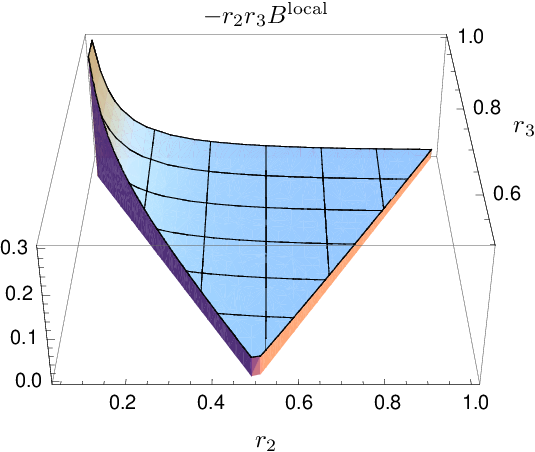
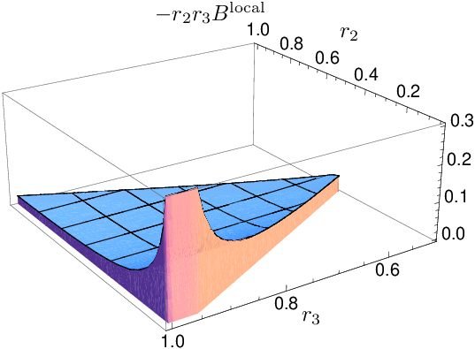
Note that by rescaling and we can pull out an overall factor and rewrite this bispectrum in terms of the two independent variables and ,
| (3.16) |
In the following we will always use this trick and plot the bispectrum as a function of and setting and . The shape corresponding to eq. (3.16) is plotted in figure 1.
|
|

|

|
3.2 The equilateral shape
Another theoretically motivated shape for the primordial 3-point function is the so-called equilateral shape, that can be described by [23]
| (3.17) |
Notice that the divergence in the squeezed limit is in this case milder than for the local shape, due to a cancellation among the various terms. We can compute the CMB bispectrum similarly to what is done in the local case. It is convenient to define
| (3.18) |
With such a definition, using eq. (3.5) for the and eq. (3.17) for the expectation value of three gravitational potentials, one finally obtains
| (3.19) |
Here and in the following we sum over all permutations of and we subsequently set . The integrals cannot be done analytically but the result is plotted in figure 2.
4 Computing the CMB bispectrum
In this section we compute the CMB bispectra due to the different second-order contributions in eq. (2.31). For comparison, we will use the two typical primordial shapes, local and equilateral, discussed above. We are only interested in computing the CMB non-Gaussianities generated in the Sachs-Wolfe limit; thus, as already mentioned, we will assume that there is no primordial non-Gaussianity, i.e. that the curvature perturbation on uniform-density hypersurfaces, , is Gaussian on super-Hubble scales. Consequently, from eq. (2.8) it follows that is Gaussian.
4.1 Intrinsic contributions at last scattering
Let us start by computing the CMB non-Gaussianity due to the second-order effects in the first line of eq. (2.31), i.e.,
| (4.1) |
This contribution has been first derived in [14] and its bispectrum and detectability have been studied in [34]. Note that, although we have dubbed it “intrinsic”, this contribution is not physically separable from the other second-order contributions integrated along the photon path that we will study below.
The momentum-independent quadratic term, , gives a contribution to the bispectrum exactly of the local shape, equivalent to [14], in eq. (3.16). Its contribution does not vanish in the equilateral limit. We can compare it to an equilateral contribution by evaluating its bispectrum in the equilateral configuration. We find
| (4.2) |
where we have evaluated for . We conclude that this contribution is equivalent to in the equilateral limit.
In order to compute the contribution from the momentum-dependent term, we rewrite it as
| (4.3) |
where is a kernel defined as
| (4.4) |
Note that this kernel vanishes in the limit of either or going to zero. Thus, we expect this contribution to be suppressed with respect to the local shape in the squeezed limit.
The Fourier transform in the sky of this contribution is
| (4.5) |
To compute the bispectrum we can contract this contribution, which is quadratic in , with the product of two linear Sachs-Wolfe effects, whose are given by eq. (3.5). By doing so, evaluating the 4-point function of using Wick’s theorem and the definition of the power spectrum, eq. (3.7), summing over all permutations, and using the definition of the bispectrum, eq. (3.8), one obtains
| (4.6) |
The integrals in the expression above can be integrated numerically. The final result for the bispectrum coming from this contribution is plotted in figure 3. Its contribution is equivalent to .

|

|
Notice that this bispectrum is suppressed in the squeezed limit with respect to the local case in figure 1. This, as discussed, is a consequence of the derivatives in eq. (4.1). Notice also that the suppression, in the limit , is linear in as there is one derivative acting on each in eq. (4.1). Thus, in the plots (which include a measure ) the function goes to a constant. This constant depends on the orientation between the long wavelength mode and the short ones as it is clear from eq. (4.4): indeed, in the figure we see that the limit depends on the direction from which the limit is approached. Notice that this behaviour is different from the case of primordial equilateral non-Gaussianity where there is a suppression going like in the squeezed limit – diverges logarithmically for , see eq. (3.19) – so that the plot in figure 2 goes to zero. Indeed, in this limit the 3d kernel (3.17) is suppressed by two powers of with respect to the local shape and this behavior is typical of all equilateral models [35, 23].
4.2 Contribution from the Rees-Sciama effect
At second-order in the perturbations, the Newtonian and curvature potentials and have a constant and a time-dependent part. While the constant part given in the first line of eqs. (2.4) and (2.5) dominates on large scales, on sub-Hubble scales one recovers the standard Newtonian limit [36], i.e. the two potentials become equal, , and grow as the scale factor, , where we have used . Thus, we expect the photon frequency to be affected by an integrated effect. This is the so-called Rees-Sciama effect [37], given by
| (4.7) |
Its contribution to the CMB bispectrum has already been considered in [20, 21] although these analysis were restricted only to the diagonal terms of the bispectrum. More generally, the bispectrum from the Rees-Sciama effect has been studied in [38].44 4 As there is an error in the derivation of eq. (23) of [38], our results cannot be compared with that reference.
Symmetrizing over the momenta, we can rewrite the integrand in eq. (4.7) as
| (4.8) |
where is an explicitly time-dependent kernel derived from eqs. (2.4) and (2.5) defined as
| (4.9) |
Note that we have multiplied it by to make it dimensionless. The Fourier transform in the sky of this contribution is given by
| (4.10) |
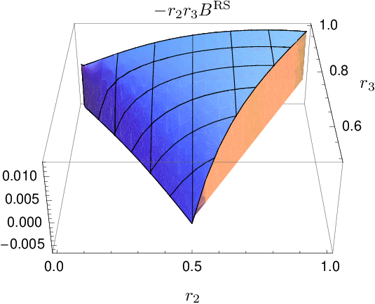
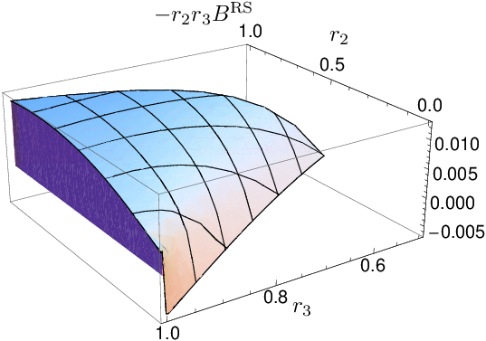
As done for the intrinsic contribution, in order to compute the bispectrum we need to contract in the above equation with the product of two linear Sachs-Wolfe effects, whose are given by eq. (3.5). Note, however, that the Rees-Sciama kernel in eq. (4.9) is higher order in the spatial gradients with respect to the intrinsic kernel of eq. (4.4), so that one may think that its contribution to the bispectrum will be relevant only on short scales. Indeed, since we are correlating the Rees-Sciama effect with the linear Sachs-Wolfe effect, which takes place at the last scattering surface, one may naively conclude that its contribution to the bispectrum is suppressed in the limit of large angles, i.e. in the limit where gradients are much smaller than the Hubble rate at decoupling. However, this is not the case. Indeed, the correlation with what happens at the last scattering surface does not vanish immediately for , but for a given mode , it remains large for and after that decays exponentially. In other words the correlation decays when the distance from the last scattering surface is of the order of the typical wavelength. In appendix A we explain better this point with a simple example. Now, since the Rees-Sciama effect grows with , the contribution to the bispectrum will be maximal for . Using that one has that the maximal contribution comes for so that the gradients are not suppressed at and one expects the Rees-Sciama contribution to the bispectrum to be of the same order as one of the intrinsic terms. Notice also that, as for the intrinsic kernel, also the kernel (4.9) vanishes in the limit of either or going to zero; we thus expect the Rees-Sciama bispectrum to be suppressed in the squeezed limit with respect to the local shape.
Let us move to the explicit calculation. It is convenient to define
| (4.11) |
By contracting given by eq. (4.10) with the product of two linear contributions given by eq. (3.5), using Wick’s theorem and the definition of the power spectrum, eq. (3.7), to rewrite the 4-point function of , and summing over all permutations one obtains, by using the variables and ,
| (4.12) |
Actually the result of the calculation is not proportional to as in the definition of eq. (3.8), but to and permutations, as a consequence of the fact that we are correlating effects at different conformal times . This is a bit surprising as the delta function is just a consequence of translational invariance. However, the discussion above implies that the bispectrum is exponentially suppressed when the triangle in Fourier space does not close, i.e. when . This can be checked explicitly in the expression (4.12). In appendix A we discuss a simple example in which this issue is made more transparent.
The above integrals are particularly challenging even numerically. However, some simplifications can be made. Since the integrand is exponentially suppressed for by the rapid oscillations of , one can push the upper limit of the integral in to . Another simplification consists in neglecting in the first integral of eq. (4.12), which is justified by the fact that we consider only modes well outside the Hubble radius at recombination and thus . With these approximations eq. (4.12) can be rewritten as
| (4.13) |
We see that the bispectrum induced by the Rees-Sciama effect goes as and it is parametrically similar to the intrinsic contribution discussed in the previous section. The analytical and numerical study of this expression is postponed to appendix B. The final result for the bispectrum is given in figure 4.
As for the intrinsic contribution (4.6), in the squeezed limit the Rees-Sciama bispectrum is suppressed when compared with the local shape by , with a coefficient which depends on the angle. We show this analytically in appendix B. By comparing the Rees-Sciama bispectrum to the equilateral contribution, as we did for the intrinsic one, we find that the Rees-Sciama contribution is equivalent to .
|
|
4.3 Integrated vector contribution
At second order, the non-diagonal part of the metric becomes non-vanishing and time dependent on sub-Hubble scales. Similarly to the time-dependent part of the gravitational potentials, it induces an integrated effect on the photon redshift, given in eq. (2.31) by
| (4.14) |
As is transverse we refer to this effect as the integrated vector contribution. As for the Rees-Sciama, to compute the bispectrum we need to correlate this integrated effect with the intrinsic temperature fluctuation at last scattering. Even though this effect is suppressed at last scattering, when modes are still out of the Hubble radius, it will give us a contribution to of order unity, similarly to what happens for the Rees-Sciama effect.
Note that the second term in the kernel (4.16) is proportional to . Thus, it is a time total derivative which can be trivially integrated in in eq. (4.14). Therefore we have another term evaluated at last scattering, analogous to the intrinsic contributions studied in section 4.1, of the form
| (4.17) |
This shows clearly that there is nothing really intrinsic about the contributions discussed in section 4.1: the splitting among the various effects is gauge dependent and only the total sum has a well defined gauge invariant meaning.
One can then split the rest of the kernel orthogonally to and along the line of sight. Indeed, decomposing into the parts orthogonal and parallel to the line of sight as , the first term in eq. (4.16) can be rewritten as
| (4.18) |
The first term of this expression is proportional to . Thus, it is higher order in with respect to the second term and therefore negligible in the flat-sky approximation. Thus, the Fourier transform on the sky of the contribution (4.18) can be approximated with
| (4.19) |
Proceeding as in the case of the intrinsic and Rees-Sciama contributions, the total contribution from vectors can be written, using the variables and , as
| (4.20) |
The first piece, which is not integrated in , comes from eq. (4.17), while the other term describes the contribution integrated along the line of sight. The integral over time can be dealt with as in the Rees-Sciama case: see appendix B. The final result for this bispectrum is given in figure 5. Again, the result is suppressed with respect to the local shape in the squeezed limit because the kernel (4.16) vanishes when either or go to zero. The behaviour in this limit is qualitatively the same as in the Rees-Sciama case. This vector contribution is equivalent to in the equilateral configuration.
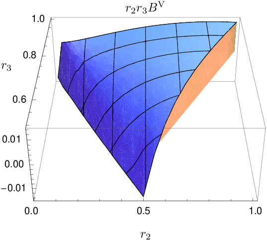
|
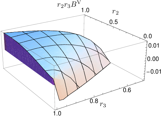
|
4.4 Integrated tensor contribution
At second order, even in the absence of primordial gravitational waves, the part of the spatial metric not proportional to the identity matrix, , is non-vanishing and time dependent on sub-Hubble scales. Thus, it induces an integrated effect given by
| (4.21) |
which we expect to contribute to the bispectrum similarly to what happens for the vectors. As is transverse and traceless, we refer to this effect as the tensor contribution. From eq. (2.7) and using eqs. (2.11) and (2.12) to rewrite the transverse traceless projector, the integrand is
| (4.22) |
where the kernel is defined as
| (4.23) |
and is a spherical Bessel function that appears from taking the time derivative of ,
| (4.24) |
As we did for the vector kernel , can be decomposed into a part parallel and orthogonal to the sky. The parallel part is higher order in and thus negligible in the flat-sky approximation. Thus, the kernel can be approximated as
| (4.25) |
The Fourier transform on the sky of this contribution is given by
| (4.26) |
With this simplification the time integral can be analytically computed and yields, expressing it in terms of the variables , and ,
| (4.27) |
plus an imaginary term odd under which does not contribute to the integral. This gives for the bispectrum
| (4.28) |
and the final result is plotted in figure 6. Again, given that the kernel (4.25) goes to zero when either or go to zero, this shape is suppressed with respect to the local one in the squeezed limit. From figure 6 we see that the integrated tensor contribution is qualitatively similar to the intrinsic kernel, Rees-Sciama and vector contributions discussed previously. This contribution is equivalent to for an equilateral configuration.

|

|
4.5 Lensing
The deflection angle of a light ray as it propagates from the last scattering surface to us is given by eq. (2.32) (for a review of lensing effects on the CMB see [39]). For convenience we reproduce it here,
| (4.29) |
The geometrical weight tells us that the effect is suppressed close to the last scattering surface. For this reason, usually the main contribution to the 3-point function due to lensing comes from the correlation of the photon deflection with the ISW [4, 5]. This effect is absent in our case as we are studying a universe with only matter. However, there is still the correlation of the intrinsic temperature fluctuation at last scattering with the lensing contribution given by
| (4.30) |
Similarly to the other integrated effects also this will give an effective .
Let us compute the contribution to the bispectrum. Inserting the deviation angle (4.29) into eq. (4.30) and using , the lensing contribution to the temperature fluctuation can be written as
| (4.31) |
Taking the Fourier transform on the sky yields
| (4.32) |
As usual, we can compute the bispectrum by correlating this effect with the intrinsic temperature at last scattering. By doing so, we obtain
| (4.33) |
Note that here one must sum over all permutations of , including the anticyclic ones. The integrals above can be computed analytically, yielding
| (4.34) |
This result is plotted in figure 7. Alternatively, this equation can be written as
| (4.35) |

|
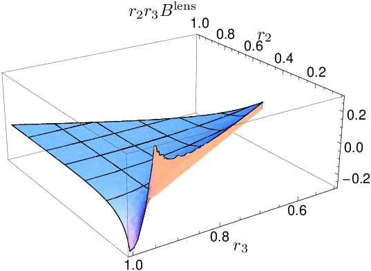
|
Another method to derive the lensing CMB bispectrum is through the lensing potential defined as (see for example [39])
| (4.36) |
The deflection angle (4.29) is obtained by taking the flat-sky gradient of this expression . The correlation between the temperature at the last scattering surface and the lensing potential is given by55 5 As explained in [39], the divergence of the lensing potential at affects only the monopole, which can always be subtracted.
| (4.37) |
The temperature fluctuation is localized at while the lensing becomes more and more important at later times. It is easy to see that the correlation is maximal at , similarly to what was discussed for all integrated effects in section 4.2 (see also appendix A).
As the integral is dominated by , we can approximate the function with to get
| (4.38) |
The bispectrum can be written as [40, 32]
| (4.39) |
which coincides with eq. (4.35).
Note that the expression in eq. (4.35) diverges in the squeezed limit. However, the form of the divergence depends on the direction one approaches the limit. One can compare the expression resulting from taking with the local form. This gives a contribution equivalent to where is the angle between and when one takes the limit. In the equilateral configuration, the lensing gives a sizable contribution, equivalent to .
It is possible to recover the lensing 3-point function in the squeezed limit in another way, which is physically more transparent and can be easily generalized to the case when the short wavelength modes are inside the horizon at recombination. We are going to calculate the 3-point function by first taking the long wavelength mode fixed and then studying its lensing effect on the short scale 2-point function.66 6 It is easy to argue that the leading contribution in the squeezed limit is obtained when the lensing mode is of long wavelength. Indeed, lensing is effective far from the last scattering surface, but as we get far from it the correlation with the temperature fluctuation rapidly decreases. The loss of correlation happens at , i.e. it is faster at high , that is why the squeezed limit is dominated by a long lensing wave. At the end we average over the long wavelength mode.77 7 This discussion is inspired by the derivation of the consistency relation for the squeezed limit of the primordial 3-point function in single field inflation [27, 41, 42]. In particular we will parallel the explicit derivation done in sec. 2 of [42]. Consider the 2-point correlation function of the temperature fluctuations in two different directions and . In the presence of a long wavelength mode the real space 2-point function is lensed
| (4.40) |
where we used the fact that the unlensed 2-point function just depends on the distance between the points. Obviously there is no effect if the two lensing angles are the same: the 2-point function is just translated. Expanding at first order and defining by and the components of and parallel to the (flat) sky we have
| (4.41) |
By assumption the lensing wave is of long wavelength so that we can evaluate the gradient of the lensing angle at the midpoint . If we call , we have
| (4.42) |
We can now Fourier transform to and . The result can be expressed in terms of and , where L and S stand for long and short wavelength,
| (4.43) |
The 3-point function is obtained multiplying the above expression by of the long wavelength mode and averaging,
| (4.44) |
The prime in the correlation between lensing and the temperature means that we have to remove the momentum conservation factor , which has been factored out.
Let us evaluate the integral over , which describes the effect of lensing on the 2-point function. One may naïvely think that for a scale invariant 2-point function, which is the case that we are studying in this paper, the effect of lensing vanishes. Indeed, the calculations above are very similar to the ones leading to the consistency relation for the squeezed limit of the primordial 3-point function [27, 41, 42]. In that case, however, the integral over does not contain the angular weight . Without this terms the integral vanishes for a scale invariant spectrum: indeed the 2-point function in real space is a logarithm of the distance, so that its log-derivative is a constant. The Fourier transform of a constant is which vanishes for any non-zero .
The situation is different in the presence of the angular weight . To be more explicit, let us introduce a scale dependence in the 2-point function and evaluate the integral in eq. (4.44) for a power spectrum of the form , which corresponds to a 2-point function going as , to see that the result does not vanish for . The integral can be written as
| (4.45) |
We see that the result does not vanish for . What vanishes for is the trace of this tensor. This means that for a scale invariant spectrum, the isotropic rescaling due to lensing does not contribute to the 3-point function. This makes sense in light of the discussion above: for the isotropic part there is no angular weight so that everything works as for the consistency relation for the squeezed limit of the primordial 3-point function [27, 41, 42]. On the other hand, the anisotropic case is similar to what happens when one calculates the primordial 3-point function of a graviton and two scalar modes, in the limit when the graviton wavelength becomes very long. The gravitational wave induces an anisotropic rescaling of the scalar 2-point function and the result does not vanish for a scale invariant spectrum [27]. An analogous effect is found when computing the contribution to the scalar trispectrum from graviton exchange [43]. In the limit where the graviton wavelength is very long, the non-isotropic rescaling induces a correlation between a pair of scalar 2-point functions. This effect has the same spin-2 angular dependence as the lensing.
Let us go back to eq. (4.44). In our case the normalization of the spectrum is given by , so that the expression of the 3-point function in the squeezed limit gives
| (4.46) |
The correlation between the temperature and the deflection angle is given by
| (4.47) |
Thus we have
| (4.48) |
In the limit , the explicit expression (4.35) gives, taking into account the permutation ,
| (4.49) |
which coincides with the expression above.
5 The total CMB bispectrum
In the previous section we have separated the calculation of the CMB bispectrum generated in the Sachs-Wolfe limit into five contributions: an intrinsic contribution expressed in terms of the Newtonian potential evaluated at last scattering, in eq. (4.6), the Rees-Sciama effect, in eq. (4.13), a contribution from the time dependence of the vector and tensor components of the metric, respectively in eqs. (4.20) and (4.28), and finally the lensing effect, in eq. (4.34). However, it is important to stress that only the sum of these contributions has a physical, gauge invariant, meaning. In this section we turn to discuss this sum, i.e. the total bispectrum. This is plotted in figure 8.

|

|
By comparing this with figure 7 one can appreciate that the lensing effect largely dominates the total bispectrum 88 8 As already stressed, the separation among different effects is gauge-dependent. Here we use the standard terminology in calling “lensing” the deflection of photons in Newtonian gauge. For a discussion about the gauge-dependence of lensing, see [39].. Let us see this more quantitatively.
In the squeezed limit the bispectrum is dominated by the intrinsic contribution and the lensing. In this limit we can compare the total bispectrum to the local bispectrum (3.16) taken with . This yields
| (5.1) |
where represents the angle between the short and long wavelength modes and . Thus, the total bispectrum corresponds to .
Note that this result can be obtained by simple arguments. As explained in section 2, the factor can be inferred using the fact that a mode still out of the Hubble radius today cannot affect a physical measurement. The angular dependent factor can be inferred by looking at the effect of a long wavelength lensing mode on the power spectrum, as explained in section 4.5.
A remark on the angular dependence in eq. (5.1) is in order here. Although it is non-vanishing in the squeezed limit, the lensing contribution (4.34) is not of the local form (3.16). In particular, as the angular dependence averages to zero, a non-Gaussianity test based on a local estimator of the form (3.16) would be almost blind to the lensing signal. A quantitative way to measure how a signal overlaps with another is provided by the cosine between two bispectra, defined as [23]
| (5.2) |
where is the scalar product between two bispectra, given by
| (5.3) | |||||
| (5.4) |
Indeed, we find that the cosine between the lensing bispectrum (4.34) and the local bispectrum (3.16) is .99 9 Note that the scalar product with the local bispectrum is logarithmically divergent for or . Thus, in order to evaluate it we have put the cutoff . For instance, one can compare this to the cosine between the local and equilateral bispectra, which is much larger, . Thus, due to the angular dependence of the squeezed limit, the lensing signal is orthogonal to the local one. We can now compare the total bispectrum to the local one. The cosine is . Thus, as it is dominated by lensing, the total bispectrum is almost orthogonal to the local signal. However, due to the term in eq. (5.1) the orthogonality is not complete and the total bispectrum slightly overlaps with the local one.
In the equilateral limit all the five contributions to the total bispectrum become important. However, the lensing numerically dominates. In this limit we can compare the total bispectrum to the equilateral bispectrum (3.19) taken with . This yields
| (5.5) |
Thus, the total bispectrum corresponds to . As it is not vanishing in the squeezed limit, its cosine with the equilateral shape will be smaller than unity. Indeed we find . Note that this value is larger than the cosine between local and equilateral shapes, i.e. . Thus, the total bispectrum is “more equilateral” than the local one. Finally, to have a confirmation that the lensing effect dominates the total bispectrum, we can compute the cosine between the total signal and the lensing. This is , which is very close to one, as expected. A summary of the cosines is given in table 1.
| Shape: | total | local | equil | lens |
|---|---|---|---|---|
| total | 1.00 | -0.17 | 0.41 | 0.98 |
| local | 1.00 | 0.30 | 0.03 | |
| equil | 1.00 | 0.47 | ||
| lens | 1.00 |
It is important to stress that the shape associated with lensing, with an angle dependent squeezed limit, represents another interesting template for the bispectrum besides the local, the equilateral and the ones studied in [44, 45]. As it is rather orthogonal to the standard local and equilateral templates, in the future it would be interesting to put limits on it, even independently of lensing.
6 Conclusion
In this paper we have calculated, assuming perfect matter dominance, the complete CMB bispectrum on large angular scales, larger than the Hubble radius at recombination, considering for the first time all the relevant effects. Although our results give the exact bispectrum in a well defined physical limit, there are many ways to improve our calculations to make them closer to the real universe. One should include the recent dark energy domination and the early transition from radiation to matter dominance along the lines of [16]. This will give qualitative new phenomena, like the rather large ISW-lensing correlation [46]. Given that we are on large angular scales, a full-sky treatment would be more precise than our flat-sky expressions, although the results for the bispectrum will be much more complicated and difficult to understand. Finally, the small deviation from a scale invariant spectrum should be included. Taking all this into account would give the correct prediction for our universe of the large angle bispectrum. This is clearly far from the complete answer. The modes on scales larger than the horizon at recombination are quite few and most of the bispectrum signal comes from triangles with modes on sub-Hubble scales. Entering in a sub-Hubble regime requires the whole machinery of second-order Boltzmann equations that we have not touched in this paper.
The calculated bispectrum is rather small: the final bispectrum is dominated by the lensing contribution, which gives , with the angle between long and short modes. Even if we could use our results on arbitrarily short scales, this would be below Planck sensitivity, limited to . This means that the bispectrum in the Sachs-Wolfe limit does not represent a relevant contamination for the forthcoming searches for primordial non-Gaussianities.
A way to go beyond the large angle regime is to correct the results of [22] to get the full bispectrum in the squeezed limit, with one (but not necessarily all) of the modes on scales larger than the horizon at recombination. We leave all these directions for future work.
Acknowledgments
It is a pleasure to thank Nicola Bartolo, Francis Bernardeau, Eiichiro Komatsu, Roy Maartens, Sabino Matarrese, Toni Riotto, Misao Sasaki, Uros Seljak, Leonardo Senatore and Matias Zaldarriaga for useful discussions. G.D’A. and P.C. thank the Institut de Physique Théorique at Saclay and F.V. thanks the ICTP for hospitality while working on this project. G.D’A., P.C., and F.V. thank the Galileo Galilei Institute, where part of this work was carried out during the workshop “New Horizons for Modern Cosmology”. Furthermore, F.V. thanks the Yukawa Institute for Theoretical Physics at Kyoto University, where part of this work was carried out during the GCOE/YITP workshop YITP-W-09-01 on “Non-linear cosmological perturbations” and the EU Marie Curie Research and Training network ”UniverseNet” (MRTN-CT-2006-035863) for support..
Appendix
Appendix A Flat-sky and integrated effects
At first order, the gravitational contribution to the temperature anisotropies in matter domination is the Sachs-Wolfe effect,
| (A.1) |
where is the unit vector specifying the line of sight direction, is the (background) conformal distance to the last scattering surface and is the first order Newtonian potential. In the flat-sky formalism [31, 32], one chooses a fiducial direction and expands at the lowest order in the angle between and :
| (A.2) |
being a 2-dimensional vector normal to . The multipole is simply the 2-dimensional Fourier transform with respect to :
| (A.3) |
One can show that the flat-sky multipole corresponds to the large limit of the full-sky one. The two are related by [32]
| (A.4) | |||
| (A.5) |
Similar expressions hold also for the power spectrum and the bispectrum. The power spectrum is defined as in flat-sky approximation, and as in full sky; the two expressions are related by for large . The bispectrum in the full and flat sky are defined respectively as
| (A.6) |
| (A.7) |
where is the Wigner 3-j symbol. The two expressions are related by:
| (A.8) |
The derivation of these expressions can be found in [32].
To better understand what happens when we correlate effects which are important at different times, we can do a simple exercise1010 10 We thank F. Bernardeau for suggesting this example.: we calculate the 2-point function of two integrated effects which peak at different times and . We will see that the correlation decays exponentially when , and that the power spectrum is proportional to up to exponentially small terms. Consider a generic integrated effect at first order:
| (A.9) |
where is a growth function. Now we correlate two such effects, with different growth functions and :
| (A.10) |
For simplicity, we approximate the growth functions with step functions, such that
| (A.11) |
where we consider . Thus we find
| (A.12) |
The integration over can be done analytically, yielding
| (A.13) |
where is the modified Bessel function, with asymptotic behaviours for and for .

We can see that, when , the correlation is exponentially suppressed. Then, in the limit we find
| (A.14) |
In general, the translational invariance in 2d is only approximate; however, the approximation is very good since for large multipoles the correlations are exponentially suppressed if the sum .
Appendix B Detailed calculation of the Rees-Sciama effect
In this appendix we compute the Rees-Sciama bispectrum. We start from eq. (4.13) before summing over cyclic permutations:
| (B.1) |
Since there are some pieces in the kernel that can be integrated analytically, we now compute them as a check of our numerical integration. To proceed, we make use of the following known integrals:
| (B.2) | ||||
| (B.3) | ||||
| (B.4) |
where the are Bessel modified functions. We then split the bispectrum into four pieces, three of which are integrated analytically:
| (B.5) |
| (B.6) |
| (B.7) |
| (B.8) |
The first three pieces can be integrated in , giving:
| (B.9) |
| (B.10) |
| (B.11) |
The fourth piece (B.8) cannot be integrated analytically, making the numerical integration necessary. However, comparison between the numerical integration of the other three pieces and the analytical expressions (B.9) to (B.11) gives consistent results. This provides a check of the validity of our computation.
Now we turn to the numerical integration of eq. (B.1). To do it we first have to perform analytically the integral, which is ill-defined. In order to overcome this problem we first change variables from , to and , and then regularize the integral in the following way:
| (B.12) |
The last integral follows from the prescription
| (B.13) |
After integrating in , we obtain:
| (B.14) |
which, after changing variables from to , and performing the derivative, gives a form which can be integrated numerically. The final results of the integration, after summing over cyclic permutations and setting , are presented in figure 4.
We can compare the Rees-Sciama contribution with the local shape in the squeezed limit. We will see that while the local shape diverges as in this limit, the Rees-Sciama only diverges as . Going back to eq. (B.1), we can study the behavior when one of the goes to zero; notice that the expression must be symmetrized so that we have to study both the limits and in eq. (B.1). For we have an infrared divergence in the integral coming from the power spectrum which goes as for . This would give a divergence as in the local model. However, for and the expression in brackets in the second line of (B.1) goes as for , but its integral vanishes due to parity, leaving only terms which are at most logarithmic divergent and thus suppressed with respect to the local shape. An additional divergence comes from the limit in eq. (B.1); in this case the integral diverges in the limit . Notice that in this case one also has to take into account the integral over which diverges for . To study the behavior for one must first integrate in using the prescription (B.12). One can see that the leading divergence in the resulting expression comes from a term of the form , which gives a divergence. This is dominant compared to the divergence in , but it is still subdominant compared to the local case. We conclude that the Rees-Sciama result is subdominant compared to the local shape in the squeezed limit. This analysis is a good check of the numerics, which indeed shows a divergence in the squeezed limit.
References
- [1] E. Komatsu et al. [WMAP Collaboration], “Five-Year Wilkinson Microwave Anisotropy Probe Observations:Cosmological Interpretation,” Astrophys. J. Suppl. 180, 330 (2009) [arXiv:0803.0547 [astro-ph]].
- [2] A. Slosar, C. Hirata, U. Seljak, S. Ho and N. Padmanabhan, “Constraints on local primordial non-Gaussianity from large scale structure,” JCAP 0808, 031 (2008) [arXiv:0805.3580 [astro-ph]].
- [3] K. M. Smith, L. Senatore and M. Zaldarriaga, “Optimal limits on from WMAP 5-year data,” arXiv:0901.2572 [astro-ph].
- [4] U. Seljak and M. Zaldarriaga, “Direct Signature of Evolving Gravitational Potential from Cosmic Microwave Background,” Phys. Rev. D 60, 043504 (1999) [arXiv:astro-ph/9811123].
- [5] D. M. Goldberg and D. N. Spergel, “Microwave background bispectrum. 2. A probe of the low redshift universe,” Phys. Rev. D 59, 103002 (1999) [arXiv:astro-ph/9811251].
- [6] R. Khatri and B. D. Wandelt, “Crinkles in the last scattering surface: Non-Gaussianity from inhomogeneous recombination,” Phys. Rev. D 79, 023501 (2009) [arXiv:0810.4370 [astro-ph]].
- [7] L. Senatore, S. Tassev and M. Zaldarriaga, “Cosmological Perturbations at Second Order and Recombination Perturbed,” arXiv:0812.3652 [astro-ph].
- [8] L. Senatore, S. Tassev and M. Zaldarriaga, “Non-Gaussianities from Perturbing Recombination,” arXiv:0812.3658 [astro-ph].
- [9] C. Pitrou, J. P. Uzan and F. Bernardeau, “Cosmic microwave background bispectrum on small angular scales,” Phys. Rev. D 78, 063526 (2008) [arXiv:0807.0341 [astro-ph]].
- [10] N. Bartolo and A. Riotto, “On the non-Gaussianity from Recombination,” JCAP 0903, 017 (2009) [arXiv:0811.4584 [astro-ph]].
- [11] N. Bartolo, S. Matarrese and A. Riotto, “CMB Anisotropies at Second-Order II: Analytical Approach,” JCAP 0701, 019 (2007) [arXiv:astro-ph/0610110].
- [12] D. Nitta, E. Komatsu, N. Bartolo, S. Matarrese and A. Riotto, “CMB anisotropies at second order III: bispectrum from products of the first-order perturbations,” arXiv:0903.0894 [astro-ph.CO].
- [13] C. Pitrou, “The radiative transfer at second order: a full treatment of the Boltzmann equation with polarization,” Class. Quant. Grav. 26, 065006 (2009) [arXiv:0809.3036 [gr-qc]].
- [14] N. Bartolo, S. Matarrese and A. Riotto, “Gauge-invariant temperature anisotropies and primordial non-Gaussianity,” Phys. Rev. Lett. 93, 231301 (2004) [arXiv:astro-ph/0407505].
- [15] N. Bartolo, S. Matarrese and A. Riotto, “Non-Gaussianity of Large-Scale CMB Anisotropies beyond Perturbation Theory,” JCAP 0508, 010 (2005) [arXiv:astro-ph/0506410].
- [16] N. Bartolo, S. Matarrese and A. Riotto, “The Full Second-Order Radiation Transfer Function for Large-Scale CMB Anisotropies,” JCAP 0605, 010 (2006) [arXiv:astro-ph/0512481].
- [17] R. K. Sachs and A. M. Wolfe, “Perturbations of a cosmological model and angular variations of the microwave background,” Astrophys. J. 147, 73 (1967).
- [18] S. Matarrese, S. Mollerach and M. Bruni, “Second-order perturbations of the Einstein-de Sitter universe,” Phys. Rev. D 58, 043504 (1998) [arXiv:astro-ph/9707278].
- [19] L. Boubekeur, P. Creminelli, J. Noreña and F. Vernizzi, “Action approach to cosmological perturbations: the 2nd order metric in matter dominance,” JCAP 0808 (2008) 028 [arXiv:0806.1016 [astro-ph]].
- [20] S. Mollerach, A. Gangui, F. Lucchin and S. Matarrese, “Contribution to the three point function of the cosmic microwave background from the Rees-Sciama effect,” Astrophys. J. 453, 1 (1995) [arXiv:astro-ph/9503115].
- [21] D. Munshi, T. Souradeep and A. A. Starobinsky, “Skewness Of Cosmic Microwave Background Temperature Fluctuations Due To Nonlinear Gravitational Instability,” Astrophys. J. 454, 552 (1995) [arXiv:astro-ph/9501100].
- [22] P. Creminelli and M. Zaldarriaga, “CMB 3-point functions generated by non-linearities at recombination,” Phys. Rev. D 70, 083532 (2004) [arXiv:astro-ph/0405428].
- [23] D. Babich, P. Creminelli and M. Zaldarriaga, “The shape of non-Gaussianities,” JCAP 0408, 009 (2004) [arXiv:astro-ph/0405356].
- [24] T. Pyne and S. M. Carroll, “Higher-Order Gravitational Perturbations of the Cosmic Microwave Background,” Phys. Rev. D 53, 2920 (1996) [arXiv:astro-ph/9510041].
- [25] S. Mollerach and S. Matarrese, “Cosmic microwave background anisotropies from second order gravitational perturbations,” Phys. Rev. D 56, 4494 (1997) [arXiv:astro-ph/9702234].
- [26] For a pedagogical introduction to Liouville’s theorem in General Relativity see C. W. Misner, K. S. Thorne and J. A. Wheeler, “Gravitation,” San Francisco 1973, 1279p.
- [27] J. M. Maldacena, “Non-Gaussian features of primordial fluctuations in single field inflationary models,” JHEP 0305, 013 (2003) [arXiv:astro-ph/0210603].
- [28] V. Acquaviva, N. Bartolo, S. Matarrese and A. Riotto, “Second-order cosmological perturbations from inflation,” Nucl. Phys. B 667, 119 (2003) [arXiv:astro-ph/0209156].
- [29] D. Langlois and F. Vernizzi, “Nonlinear perturbations of cosmological scalar fields,” JCAP 0702, 017 (2007) [arXiv:astro-ph/0610064].
- [30] W. Hu and A. Cooray, “Gravitational time delay effects on cosmic microwave background anisotropies,” Phys. Rev. D 63, 023504 (2001) [arXiv:astro-ph/0008001].
- [31] U. Seljak, “Gravitational lensing effect on cosmic microwave background anisotropies: A Power spectrum approach,” Astrophys. J. 463, 1 (1996) [arXiv:astro-ph/9505109].
- [32] W. Hu, “Weak lensing of the CMB: A harmonic approach,” Phys. Rev. D 62, 043007 (2000) [arXiv:astro-ph/0001303].
- [33] E. Komatsu et al. [WMAP Collaboration], “First Year Wilkinson Microwave Anisotropy Probe (WMAP) Observations: Tests of Gaussianity,” Astrophys. J. Suppl. 148, 119 (2003) [arXiv:astro-ph/0302223].
- [34] M. Liguori, F. K. Hansen, E. Komatsu, S. Matarrese and A. Riotto, “Testing Primordial Non-Gaussianity in CMB Anisotropies,” Phys. Rev. D 73, 043505 (2006) [arXiv:astro-ph/0509098].
- [35] P. Creminelli, “On non-gaussianities in single-field inflation,” JCAP 0310, 003 (2003) [arXiv:astro-ph/0306122].
- [36] P. J. E. Peebles, “The Large-Scale Structure of the Universe,” (Princeton Series in Physics, 1980) Princeton Univ Pr 1980, 440p.
- [37] M. J. Rees and D. W. Sciama, “Large scale Density Inhomogeneiies in the Universe,” Nature 217, 511 (1968).
- [38] D. N. Spergel and D. M. Goldberg, “Microwave background bispectrum. 1. Basic formalism,” Phys. Rev. D 59, 103001 (1999) [arXiv:astro-ph/9811252].
- [39] A. Lewis and A. Challinor, “Weak Gravitational Lensing of the CMB,” Phys. Rept. 429, 1 (2006) [arXiv:astro-ph/0601594].
- [40] M. Zaldarriaga, “Lensing of the CMB: Non-Gaussian aspects,” Phys. Rev. D 62, 063510 (2000) [arXiv:astro-ph/9910498].
- [41] P. Creminelli and M. Zaldarriaga, “Single field consistency relation for the 3-point function,” JCAP 0410, 006 (2004) [arXiv:astro-ph/0407059].
- [42] C. Cheung, A. L. Fitzpatrick, J. Kaplan and L. Senatore, “On the consistency relation of the 3-point function in single field inflation,” JCAP 0802, 021 (2008) [arXiv:0709.0295 [hep-th]].
- [43] D. Seery, M. S. Sloth and F. Vernizzi, “Inflationary trispectrum from graviton exchange,” JCAP 0903, 018 (2009) [arXiv:0811.3934 [astro-ph]].
- [44] P. D. Meerburg, J. P. van der Schaar and P. S. Corasaniti, “Signatures of Initial State Modifications on Bispectrum Statistics,” arXiv:0901.4044 [hep-th].
- [45] L. Senatore, K. M. Smith and M. Zaldarriaga, “Non-Gaussianities in Single Field Inflation and their Optimal Limits from the WMAP 5-year Data,” arXiv:0905.3746 [astro-ph.CO].
- [46] D. Hanson, K. M. Smith, A. Challinor and M. Liguori, “CMB lensing and primordial non-Gaussianity,” arXiv:0905.4732 [astro-ph.CO].