New Physics from Flavour

The UTfit Collaboration [1] aims to determine the coordinates $\bar{\rho}$ and $\bar{\eta}$ of the apex of the Unitarity Triangle (UT), and in general the elements of the CKM matrix [2] in the Standard Model (SM). Nowadays the SM analysis includes many experimental and theoretical results, such as predictions for several flavour observables and measurements of hadronic parameters which can be compared with the lattice QCD predictions [3]. More recently, the UT analysis has been extended beyond the SM, allowing for a model-independent determination of $\bar{\rho}$ and $\bar{\eta}$ — assuming negligible New Physics (NP) contributions to tree-level processes — and a simultaneous evaluation of the size of NP contributions to $\Delta F=2$ amplitudes compatible with the flavour data [4, 5]. Recently, the NP analysis has been expanded to include an effective field theory study of the allowed NP contributions to $\Delta F=2$ amplitudes. This allows one to put model-independent bounds on the NP energy scale associated to flavour- and CP-violating phenomena [6].

In these proceedings we present a preliminary update of our UT analysis in the SM, including a set of fit predictions and a study of the compatibility between the fit results and some of the most interesting experimental constraints. The main difference with respect to previously published results comes from the use of an updated set of lattice QCD results [7] and of some constraints ($\bar{m}_{t}$, $\alpha$, $\gamma$, $|V_{ub}|$) updated to the latest available measurements. We also show an update of the analysis beyond the SM, with particular emphasis on NP contributions to the $B_{s}$ mixing phase, where we observe a significant discrepancy with respect to the SM prediction.

In the UT analysis we combine the available theoretical and experimental information relevant to determine $\bar{\rho}$ and $\bar{\eta}$. To this end, we use a Bayesian approach as described in ref. [8]. The theoretical and experimental input values and errors are collected in Table 1.

The results of the SM fit are shown in Table 2, while the $\bar{\rho}$–$\bar{\eta}$ plane can be found in Figure 1, where the $68\%$ and $95\%$ probability regions are plotted together with the $95\%$ regions selected by the single constraints. It is quite remarkable that the overall picture looks very consistent. The parameters $\bar{\rho}$ and $\bar{\eta}$ are determined in the SM with a relative errors of $14\%$ and $4\%$ respectively.

Within the precision of $\sim 5$–$10\%$, the CKM mechanism of the SM is able to describe pretty well the violation of the CP symmetry. In addition, flavour-changing CP-conserving and CP-violating processes select compatible regions in the $\bar{\rho}$–$\bar{\eta}$ plane, as predicted by the three-generation unitarity. This is illustrated on the left side of fig. 2, while on the right side we show the constraining power of the CP-violating observables (namely the UT angles) in the $B_{d}$ sector only.

The results of the fit are displayed in Table 2. In order to check the compatibility of the various measurements with the results of the fit, we make a comparison of the fit prediction obtained without using the observable of interest as an input and the experimental measurement. Such predictions for a subset of observables are collected in Table 3.

The two most significant discrepancies between measurements and fit predictions concern $\sin 2\beta$ and the inclusive determination of $|V_{ub}|$. As can be seen in fig. 3, they are at the level of $\sim 1.5\sigma$, showing the excellent overall compatibility of the measurements with the SM fit (with the remarkable exception of the $B_{s}$ mixing phase, as we will see in the following).

The measured value of $\sin 2\beta$ is $1.5\sigma$ smaller than the fitted one. Comparing with the results of refs. [9, 10], we find that the SM fit using constraints from $|V_{ub}|$, $\varepsilon_{K}$ and $\Delta m_{s}$/$\Delta m_{d}$ only is again $1.5\sigma$ larger than the measurement, using the input values of Table 1.

Once it is established that the CKM mechanism is the main source of CP violation so far, an accurate model-independent determination of $\bar{\rho}$ and $\bar{\eta}$ is extremely important for identifying NP in the flavour sector.

The generalized UT fit, using only $\Delta F=2$ processes and parametrizing generic NP contributions, allows for the model-independent determination of $\bar{\rho}$ and $\bar{\eta}$ under the assumptions of negligible tree-level NP contributions. Details of the method can be found in ref. [4].

A peculiar prediction of the SM is that CP violation in $B_{s}$ mixing should be very small. For this reason, the experimental observation of a sizable CP violation in $B_{s}$ mixing would be an unambiguous signal of NP.

In fact, the present data give a hint of a $B_{s}$ mixing phase much larger than expected in the SM, with a significance at about $3\sigma$ [5]. This result is obtained by combining all available experimental information with the method used by our collaboration for UT analyses.

We perform a model-independent analysis of NP contributions to $B_{s}$ mixing using the following parameterization [6]:

where $H_{\mathrm{eff}}^{\mathrm{full}}$ is the effective Hamiltonian generated by both SM and NP, while $H_{\mathrm{eff}}^{\mathrm{SM}}$ only contains SM contributions. The angle $\beta_{s}$ is defined as $\beta_{s}=\arg(-(V_{ts}V_{tb}^{*})/(V_{cs}V_{cb}^{*}))$ and it equals $0.018\pm 0.001$ in the SM.

We make use of the following experimental inputs: the CDF measurement of $\Delta m_{s}$ [12], the semi-leptonic asymmetry in $B_{s}$ decays $A_{\mathrm{SL}}^{s}$ [13], the di-muon charge asymmetry $A_{\mathrm{SL}}^{\mu\mu}$ from DØ [14] and CDF [15], the measurement of the $B_{s}$ lifetime from flavour-specific final states [16], the two-dimensional likelihood ratio for $\Delta\Gamma_{s}$ and $\phi_{s}=2(\beta_{s}-\phi_{B_{s}})$ from the time-dependent tagged angular analysis of $B_{s}\to J/\psi\phi$ decays by CDF [17] and the correlated constraints on $\Gamma_{s}$, $\Delta\Gamma_{s}$ and $\phi_{s}$ from the same analysis performed by DØ [18]. For the latter, since the complete likelihood is not available yet, we start from the results of the $7$-variable fit in the free-$\phi_{s}$ case from Table I of ref. [18]. We implement the $7\times 7$ correlation matrix and integrate over the strong phases and decay amplitudes to obtain the reduced $3\times 3$ correlation matrix used in our analysis. In the DØ analysis, the twofold ambiguity inherent in the measurement ($\phi_{s}\to\pi-\phi_{s}$, $\Delta\Gamma_{s}\to-\Delta\Gamma_{s}$, $\cos\delta_{1,2}\to-\cos\delta_{1,2}$) for arbitrary strong phases was removed using a value for $\cos\delta_{1,2}$ derived from the BaBar analysis of $B_{d}\to J/\Psi K^{*}$ using SU(3). However, this neglects the singlet component of $\phi$ and, although the sign of $\cos\delta_{1,2}$ obtained using SU(3) is consistent with the factorization estimate, to be conservative we reintroduce the ambiguity in the DØ measurement, taking the errors quoted by DØ as Gaussian and duplicate the likelihood at the point obtained by applying the discrete ambiguity. Hopefully DØ will present results without assumptions on the strong phases in the future, allowing for a more straightforward combination. Finally, for the CKM parameters we perform the UT analysis in the presence of arbitrary NP as described in ref. [6], obtaining $\overline{\rho}=0.141\pm 0.036$ and $\overline{\eta}=0.373\pm 0.028$.

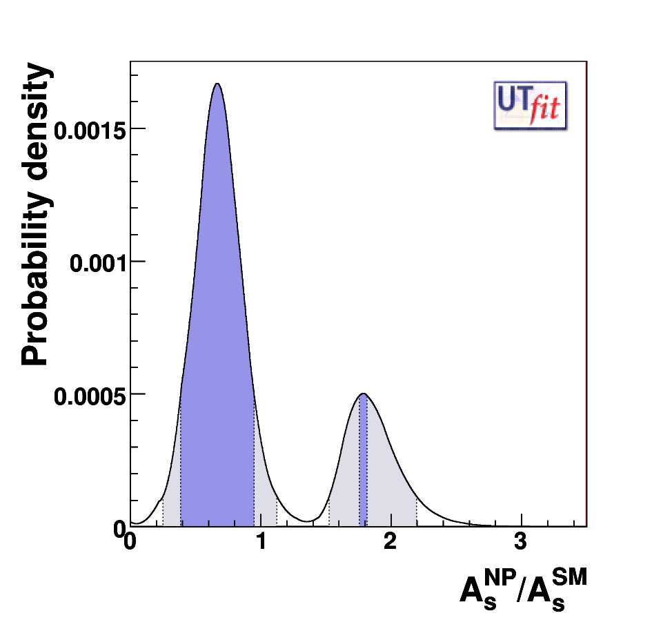
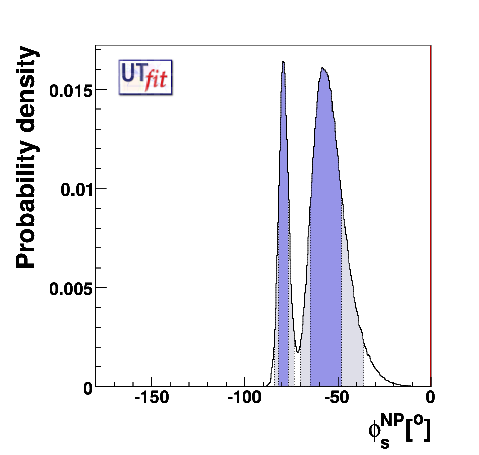
The results of our analysis are summarized in Table 4. We see that the phase $\phi_{B_{s}}$ deviates from zero at more than $3.0\sigma$. In Fig. 4 we present the two-dimensional $68\%$ and $95\%$ probability regions for the NP parameters $C_{B_{s}}$ and $\phi_{B_{s}}$, the corresponding regions for the parameters $A^{\mathrm{NP}}_{s}/A^{\mathrm{SM}}_{s}$ and $\phi^{\mathrm{NP}}_{s}$, and the one-dimensional distributions for NP parameters.

The solution around $\phi_{B_{s}}\sim-20^{\circ}$ corresponds to $\phi^{\mathrm{NP}}_{s}\sim-56^{\circ}$ and $A^{\mathrm{NP}}_{s}/A^{\mathrm{SM}}_{s}\sim 79\%$. The second solution is much more distant from the SM and it requires a dominant NP contribution ($A^{\mathrm{NP}}_{s}/A^{\mathrm{SM}}_{s}\sim 180\%$) and in this case the NP phase is very well determined.

Finally, we have tested the significance of the NP signal against different modeling of the probability density function (p.d.f.). We have explored two more methods with respect to the standard Gaussian one used by the DØ Collaboration in presenting the result: this is mainly to address the non-Gaussian tails that the experimental likelihood is showing. Firstly, we have used the $90\%$ C.L. range for $\phi_{s}=[-0.06,1.20]^{\circ}$ given by DØ to estimate the standard deviation, obtaining $\phi_{s}=(0.57\pm 0.38)^{\circ}$ as input for the Gaussian analysis. This is conservative since the likelihood has a visibly larger half-width on the side opposite to the SM expectation (see Fig. 2 of Ref. [18]). Second, we have implemented the likelihood profiles for $\phi_{s}$ and $\Delta\Gamma_{s}$ given by DØ, discarding the correlations but restoring the strong phase ambiguity. The likelihood profiles include the second minimum corresponding to $\phi_{s}\to\phi_{s}+\pi$, $\Delta\Gamma\to-\Delta\Gamma$, which is disfavoured by the oscillating terms present in the tagged analysis and is discarded in the Gaussian analysis. Also this approach is conservative since each one-dimensional profile likelihood is minimized with respect to the other variables relevant for our analysis. It is remarkable that both methods give a deviation of $\phi_{B_{s}}$ from zero of $3\,\sigma$. We conclude that the combined analysis gives a stable departure from the SM, although the precise number of standard deviations depends on the procedure followed to combine presently available data.

References

- [1] UTfit Collaboration, http://www.utfit.org.
- [2] N. Cabibbo, Phys. Rev. Lett. 10 (1963) 531; M. Kobayashi and T. Maskawa, Prog. Theor. Phys. 49, 652 (1973).
- [3] M. Bona et al. [UTfit Collaboration], JHEP 0507, 028 (2005) [arXiv:hep-ph/0501199]; M. Bona et al. [UTfit Collaboration], JHEP 0610, 081 (2006) [arXiv:hep-ph/0606167].
- [4] M. Bona et al. [UTfit Collaboration], JHEP 0603, 080 (2006) [arXiv:hep-ph/0509219]; M. Bona et al. [UTfit Collaboration], Phys. Rev. Lett. 97, 151803 (2006) [arXiv:hep-ph/0605213].
- [5] M. Bona et al. [UTfit Collaboration], arXiv:0803.0659 [hep-ph].
- [6] M. Bona et al. [UTfit Collaboration], JHEP 0803, 049 (2008) [arXiv:0707.0636 [hep-ph]].
- [7] V. Lubicz and C. Tarantino, arXiv:0807.4605 [hep-lat].
- [8] M. Ciuchini et al., JHEP 0107, 013 (2001) [arXiv:hep-ph/0012308].
- [9] E. Lunghi and A. Soni, Phys. Lett. B 666, 162 (2008) [arXiv:0803.4340 [hep-ph]].
- [10] A. J. Buras and D. Guadagnoli, Phys. Rev. D 78 (2008) 033005 [arXiv:0805.3887 [hep-ph]].
- [11] M. Bona et al. [UTfit Collaboration], JHEP 0507, 028 (2005); M. Bona et al. [UTfit Collaboration], JHEP 0610, 081 (2006).
- [12] A. Abulencia et al. [CDF Collaboration], Phys. Rev. Lett. 97, 242003 (2006).
- [13] V. M. Abazov et al. [D0 Collaboration], Phys. Rev. Lett. 98, 151801 (2007).
- [14] V. M. Abazov et al. [D0 Collaboration], Phys. Rev. D 74, 092001 (2006).
- [15] CDF Collaboration, CDF note 9015.
- [16] D. Buskulic et al. [ALEPH Collaboration], Phys. Lett. B 377, 205 (1996); F. Abe et al. [CDF Collaboration], Phys. Rev. D 59, 032004 (1999); P. Abreu et al. [DELPHI Collaboration], Eur. Phys. J. C 16, 555 (2000); K. Ackerstaff et al. [OPAL Collaboration], Phys. Lett. B 426, 161 (1998); V. M. Abazov et al. [D0 Collaboration], Phys. Rev. Lett. 97, 241801 (2006); CDF Collaboration, CDF note 7386; CDF Collaboration, CDF note 7757; E. Barberio et al. [HFAG], arXiv:hep-ex/0603003; CDF Collaboration, CDF note 9203.
- [17] T. Aaltonen et al. [CDF Collaboration], arXiv:0712.2397 [hep-ex].
- [18] V. M. Abazov et al. [D0 Collaboration], arXiv:0802.2255 [hep-ex].