Moving NRQCD for heavy-to-light form factors on the lattice

Preprint: DAMTP-2008-113Preprint: Edinburgh 2008/27

R. R. Horgan Affiliation: Department of Applied Mathematics and Theoretical Physics, University of Cambridge, Centre for Mathematical Sciences, Cambridge CB3 0WA, United Kingdom L. Khomskii Affiliation: Department of Applied Mathematics and Theoretical Physics, University of Cambridge, Centre for Mathematical Sciences, Cambridge CB3 0WA, United Kingdom S. Meinel Affiliation: Department of Applied Mathematics and Theoretical Physics, University of Cambridge, Centre for Mathematical Sciences, Cambridge CB3 0WA, United Kingdom M. Wingate Affiliation: Department of Applied Mathematics and Theoretical Physics, University of Cambridge, Centre for Mathematical Sciences, Cambridge CB3 0WA, United Kingdom K. M. Foley Affiliation: Laboratory for Elementary-Particle Physics, Cornell University, Ithaca, NY 14853, U.S.A. G. P. Lepage Affiliation: Laboratory for Elementary-Particle Physics, Cornell University, Ithaca, NY 14853, U.S.A. G. M. von Hippel Affiliation: Deutsches Elektronen-Synchroton DESY, Platanenallee 6, 15738 Zeuthen, Germany A. Hart Affiliation: SUPA, School of Physics and Astronomy, University of Edinburgh, King’s Buildings, Mayfield Road, Edinburgh EH9 3JZ, United Kingdom E. H. Müller Affiliation: SUPA, School of Physics and Astronomy, University of Edinburgh, King’s Buildings, Mayfield Road, Edinburgh EH9 3JZ, United Kingdom C. T. H. Davies Affiliation: SUPA, Department of Physics and Astronomy, University of Glasgow, Glasgow G12 8QQ, United Kingdom A. Dougall Affiliation: SUPA, Department of Physics and Astronomy, University of Glasgow, Glasgow G12 8QQ, United Kingdom K. Y. Wong Affiliation: SUPA, Department of Physics and Astronomy, University of Glasgow, Glasgow G12 8QQ, United Kingdom HPQCD Collaboration Affiliation:

Abstract

We formulate Non-Relativistic Quantum Chromodynamics (NRQCD) on a lattice which is boosted relative to the usual discretization frame. Moving NRQCD (mNRQCD) allows us to treat the momentum for the heavy quark arising from the frame choice exactly. We derive mNRQCD through $\mathcal{O}(1/m^{2},v_{\operatorname{rel}}^{4})$ , as accurate as the NRQCD action in present use, both in the continuum and on the lattice with $\mathcal{O}(a^{4})$ improvements. We have carried out extensive tests of the formalism through calculations of two-point correlators for both heavy-heavy (bottomonium) and heavy-light ( $B_{s}$ ) mesons in 2+1 flavor lattice QCD and obtained nonperturbative determinations of energy shift and external momentum renormalization. Comparison to perturbation theory at $\mathcal{O}(\alpha_{s})$ is also made. The results demonstrate the effectiveness of mNRQCD. In particular we show that the decay constants of heavy-light and heavy-heavy mesons can be calculated with small systematic errors up to much larger momenta than with standard NRQCD.

pacs

12.38.Bx, 12.38.Gc, 12.39.Hg, 13.20.He, 14.40.Nd, 14.65.Fy

I Introduction

The Cabibbo-Kobayashi-Maskawa (CKM) matrix is the focus of intense study; an inconsistency between independent determinations of CKM matrix elements from different physical processes would be evidence for new physics beyond the Standard Model. While experimental measurements of exclusive semileptonic decays have reached good precision and will be improved further by LHCb, determinations of CKM matrix elements from the decay rates are complicated by the need for precise theoretical calculations in nonperturbative quantum chromodynamics (QCD). Lattice QCD provides a first-principles approach to these calculations and it is important to reduce systematic and statistical errors as far as possible.

For example, the decay $B\rightarrow\pi\ell\nu$ [1, 2, 3] can be used to determine the CKM matrix element $V_{ub}$ while the rare decays $B\rightarrow K^{*}\gamma,~K^{(*)}\ell^{+}\ell^{-}$ [4, 5, 6, 7, 8] provide excellent opportunities to study contributions from new physics, as the flavor-changing neutral current $b\rightarrow s$ is loop-suppressed in the Standard Model. In both cases, a nonperturbative calculation of the hadronic form factors is required.

These form factors are a function of the momentum transfer squared, $q^{2}$ , where $q=p_{B}-p_{F}$ is the difference between the four-momenta of the $B$ meson and the meson in the final state. If this meson is light compared to the $B$ meson, the recoil momentum at small values of $q^{2}$ can be very large. Unfortunately, current lattice QCD calculations of these form factors work well only for low recoil momenta, i.e. large $q^{2}$ [9, 10, 11, 12], while for $B\rightarrow K^{*}\gamma$ one has $q^{2}=0$ and experimental data for $B\rightarrow\pi\ell\nu$ covers the full $q^{2}$ range [1, 2, 3].

By computing at just one or a few points with large $q^{2}$ , one might be able to reduce the error on $|V_{ub}|$ from $B\to\pi\ell\nu$ , where the shape of the form factor is now being measured precisely by experiment [1, 2, 3]. However, the form factors governing the rare $b\to s$ decays are not well-determined and must be computed using lattice QCD. Given the propensity for models of new physics to introduce new sources of flavor-changing neutral currents, it is desirable to have new tools to reduce the errors on the Standard Model calculations of differential cross sections for rare decays.

In this paper we present a technique for extending lattice QCD calculations of the decays of mesons containing one heavy quark to lower $q^{2}$ values than has hitherto been possible by reducing the discretization errors owing to the large recoil of the final state meson.

The formalism that we describe and put to the test in subsequent sections is a generalization of Non-Relativistic QCD (NRQCD) [13, 14]. The NRQCD formalism, which has already had considerable success in the study of heavy-quark systems, relies on the fact that fluctuations in the heavy quark momentum within a heavy meson are small compared with the mass of the meson itself. The Lagrangian of NRQCD is expressed as a sum over operators whose importance is governed by power-counting rules; in dimensionless units the operators are ordered in powers of $g,v_{\operatorname{rel}}$ for heavy-heavy mesons and in powers of $\alpha_{s},\Lambda_{\mathrm{QCD}}/m$ for heavy-light mesons, where $\alpha_{s}=g^{2}/(4\pi)$ is the strong coupling constant, $v_{\operatorname{rel}}\sim|{\boldsymbol{p}}|/m$ is the relative internal velocity of the heavy quarks and $m$ is the heavy quark mass.¹¹ 1 These rules are frequently referred to as NRQCD and HQET power counting schemes, respectively. Note that the choice of NRQCD as a lattice action is compatible with both schemes. See Sec. III.2 below. For NRQCD, the heavy meson is usually taken to be at rest in the lattice frame. This is appropriate for calculations of the mass spectrum of heavy-light and heavy-heavy mesons and for zero-recoil or low-recoil decays. However, for the heavy-to-light decays of the $B$ -meson cited above, outside the low recoil region the momentum of the light meson in the final state becomes comparable to the inverse lattice spacing. Consequently the calculation is sensitive to lattice artifacts which lead to large systematic errors.

It is therefore better to give the $B$ meson a non-zero momentum in the opposite direction, thereby reducing the final meson’s momentum at a given $q^{2}$ . To substantially reduce the momentum of the final meson, the momentum of the $B$ meson has to be very large, so that NRQCD would no longer be able to describe the $b$ quark inside it due to relativistic and lattice spacing errors. However, we note that fluctuations of momentum of the heavy quark inside the $B$ meson are much smaller than the momentum of the meson itself. Therefore, to reduce errors, instead of discretizing the momentum of the $b$ quark itself, we choose to discretize its fluctuations inside the moving $B$ meson. The formalism which achieves this goes by the name of moving NRQCD (mNRQCD) in which the expansion is about the state where the heavy quark is moving with a velocity $v$ , the frame velocity; this formalism was introduced briefly in [15]; Earlier, related approaches were proposed in [16, 17].

The remainder of the paper is structured as follows. In Section II we discuss the choice of the optimal reference frame for the lattice calculations. We give an explicit derivation of the continuum mNRQCD action in Section III. We explain how the theory is discretized in Section IV. In Section V we develop perturbative methods for mNRQCD and explain how to derive the renormalization of parameters due to radiative corrections. We give 1-loop results for the heavy quark renormalization constants. The construction of decay currents is discussed in section V.4. Then, in section VI we present the results of nonperturbative calculations based on two-point correlators for heavy-heavy and heavy-light mesons in mNRQCD. These include the spectrum, renormalization constants and decay constants for various values of the frame velocity $v$ .

The perturbative and nonperturbative renormalization constants are compared in Section VII. We summarize and discuss our results in Section VIII.

In the Appendices we specify some notation (Appendix A), describe the removal of time derivatives in the $\mathcal{O}(\Lambda_{\mathrm{QCD}}^{2}/m^{2})$ mNRQCD Hamiltonian (Appendix B), give explicit expressions for the lattice derivative operators (Appendix C) and tadpole improvement corrections (Appendix D) and present further perturbative results for a set of simpler actions (Appendix E). We comment on the poles of the Symanzik-improved gluon action in Appendix F.

Preliminary versions of this work have been presented in Refs. [18, 19, 20, 21, 22, 23].

II Minimizing Errors

We start by parametrizing the 4-momentum of the $b$ quark as

p=m\>u+k

where $m$ is the mass of the $b$ -quark, and $u$ a 4-velocity. In traditional (non-moving) NRQCD one has $u=(1,0,0,0)$ , and a non-relativistic expansion in the residual 3-momentum ${\boldsymbol{k}}$ is performed. In other words, the heavy-quark mass term is removed from the Lagrangian. Thus, the 3-momentum ${\boldsymbol{p}}$ , which is equal to ${\boldsymbol{k}}$ in this case, has to be small to prevent large relativistic errors as well as discretization errors on the lattice.

In moving NRQCD, we generalize this to other frames of reference, removing the momentum $m\,u$ with an arbitrary 4-velocity $u$ from the Lagrangian, and again performing a non-relativistic expansion in the residual 3-momentum ${\boldsymbol{k}}$ . The relativistic energy of the heavy quark is $E=\sqrt{\mathstrut{{\boldsymbol{p}}}^{2}+m^{2}}=\sqrt{(m{\boldsymbol{u}}+{\boldsymbol{k}})^{2}+m^{2}}$ . Taylor expansion for small $|{\boldsymbol{k}}|$ gives

E=\gamma m+{\boldsymbol{v}}\cdot{\boldsymbol{k}}+\frac{{\boldsymbol{k}}^{2}-({\boldsymbol{v}}\cdot{\boldsymbol{k}})^{2}}{2\gamma m}+\cdots

where we write $u=(u_{0},{\boldsymbol{u}})=(\gamma,\gamma{\boldsymbol{v}})$ with the 3-velocity ${\boldsymbol{v}}$ and $\gamma=(1-{\boldsymbol{v}}^{2})^{-1/2}$ . Discarding the constant term $\gamma m$ , we expect that the $\mathcal{O}(1/m)$ “kinetic” part of the continuum mNRQCD Hamiltonian in momentum space will be given by

H_{0}={\boldsymbol{v}}\cdot{\boldsymbol{k}}+\frac{{\boldsymbol{k}}^{2}-({\boldsymbol{v}}\cdot{\boldsymbol{k}})^{2}}{2\gamma m}.

Of course, the size of ${\boldsymbol{k}}$ and the associated relativistic and discretization errors depend on the choice of $u$ . The standard choice is $u=p_{B}/M_{B}$ , the 4-velocity of the $B$ meson. Then, the residual momentum ${\boldsymbol{k}}$ is small compared to ${\boldsymbol{p}}_{B}$ and the non-relativistic expansion in ${\boldsymbol{k}}$ is a good approximation even for $B$ mesons at moderately high velocities.

II.0.1 Discretization errors

One of the main applications of the mNRQCD approach is to the heavy-to-light weak decay of a $B$ -meson to a final state including a light meson. As discussed in the introduction the size of the discretization errors in a lattice calculation depends on the momentum of the final state meson; states with spatial momenta comparable to the inverse lattice spacing can be affected by lattice artifacts. Nevertheless, one wishes to compute matrix elements over the whole physical kinematic range, including the large recoil regime where the final state has large momentum relative to the $B$ meson. With mNRQCD we attempt to reduce discretization errors by choosing a non-zero frame velocity $v$ , so that the final state meson can have moderate spatial momentum in the lattice frame, even as we explore large recoil kinematics.

If the $B$ meson is at rest, the residual momentum ${\boldsymbol{k}}$ has a distribution with width of the order $\Lambda_{\mathrm{QCD}}$ and the residual energy has a distribution with width of the order $\Lambda_{\mathrm{QCD}}^{2}/(2m)\ll\Lambda_{\mathrm{QCD}}$ . Note that the momentum ${\boldsymbol{p}}_{\mathrm{spec}}$ of the light quark in the $B$ meson (the “spectator quark”) is of the same order by momentum conservation.

For a $B$ meson moving with velocity ${\boldsymbol{v}}$ , the momentum distribution is boosted to approximately $\gamma\Lambda_{\mathrm{QCD}}$ . Let us now consider a decay $B\rightarrow F$ where $F$ denotes the light meson in the final state and the 4-momenta are

	$\displaystyle p_{B}$	$\displaystyle=$	$\displaystyle(\gamma M_{B},\>\gamma M_{B}{\boldsymbol{v}}),$
	$\displaystyle p_{F}$	$\displaystyle=$	$\displaystyle(\sqrt{M_{F}^{2}+\|{\boldsymbol{p}}_{F}\|^{2}},\>{\boldsymbol{p}}_{F})$

where ${\boldsymbol{v}}$ is antiparallel to ${\boldsymbol{p}}_{F}$ . For a given value of $q^{2}=(p_{B}-p_{F})^{2}$ , we shall determine the optimal velocity of the $B$ meson which minimizes discretization errors. The discretization errors are determined by the momenta carried by the quarks (and gluons) and are typically proportional to $(a\times\mathrm{momentum})^{2}$ where $a$ is the lattice spacing. The full mNRQCD action described in this paper has no tree-level $\mathcal{O}(a^{2}{\boldsymbol{k}}^{2})$ -errors, but has $\mathcal{O}(\alpha_{s}a^{2}{\boldsymbol{k}}^{2})$ errors due to radiative corrections. The same is true for highly improved light quark actions such as ASQTAD [24, 25, 26] or HISQ [27]. Assuming that the constants of proportionality for the discretization errors are the same, discretization errors are minimal if all quarks involved in the decay have momenta of the same size.

The increase in discretization errors for the quarks in the $B$ meson due to the boost of the momentum distribution when going from zero velocity ( $\gamma=1$ ) to a non-zero velocity ${\boldsymbol{v}}$ is proportional to

\gamma^{2}\Lambda_{\mathrm{QCD}}^{2}-\Lambda_{\mathrm{QCD}}^{2}.

(1)

Assuming that the quarks in the light meson share the momentum equally, each carrying momentum of order ${\boldsymbol{p}}_{F}/2$ , we expect that the increase in relative discretization errors for the light meson when going from zero momentum to ${\boldsymbol{p}}_{F}$ is proportional to

\left({\textstyle\frac{1}{2}}|{\boldsymbol{p}}_{F}|\right)^{2}.

(2)

The total error is the sum of these terms with some coefficients that we presume are of order unity. Noting that $(p_{B}-p_{F})^{2}=q^{2}$ , we choose $v$ to minimize the total error to give the optimal $v$ as a function of $q^{2}$ . Investigation with different reasonable choices of coefficients shows that the minimum error is compatible with setting the two above terms equal. The result is plotted in Figure 1 for the $\pi$ , $K$ and $K^{*}$ light mesons. We find that at maximum recoil a velocity of $|{\boldsymbol{v}}|\approx 0.7$ would minimize discretization errors. Of course this is only a very crude estimate, and the optimal velocity depends on the details of the lattice computation.

Refer to caption — Figure 1: Estimate of optimal velocity, minimizing discretization errors, for $B\to F$ form factors (see text) as a function of $q^{2}$ for the $\pi$ , $K$ and $K^{*}$ light mesons.

II.0.2 Statistical errors

Lattice calculations are not only limited by discretization errors, but also by statistical errors. Unfortunately these increase exponentially when going to lower $q^{2}$ . Consider for instance the $B$ -meson two-point function with momentum ${\boldsymbol{p}}_{B}$ , denoted as $\langle B^{\dagger}({\boldsymbol{p}}_{B},0)B({\boldsymbol{p}}_{B},\tau)\rangle$ , which is required in the form factor computations alongside the pion two-point function and the $B\rightarrow F$ three-point function. The variance in the correlator is [28]

	$\displaystyle\sigma^{2}(\tau)$	$\displaystyle=$	$\displaystyle\left\langle[B^{\dagger}({\boldsymbol{p}}_{B},0)B({\boldsymbol{p}}_{B},\tau)][B^{\dagger}({\boldsymbol{p}}_{B},0)B({\boldsymbol{p}}_{B},\tau)]^{\dagger}\right\rangle$		(3)
			$\displaystyle-\left\|\langle B^{\dagger}({\boldsymbol{p}}_{B},0)B({\boldsymbol{p}}_{B},\tau)\rangle\right\|^{2}.$		(3)

The correlator in the first line of (3) couples to the combination of a heavy-heavy (HH) meson at rest and a pion at rest, so for large Euclidean time $\tau$ , it will decay like $\exp(-(M_{HH}+M_{\pi})\tau)$ . However, the second line is simply the square of the two-point function, which will decay like $\exp(-2E_{B}({\boldsymbol{p}}_{B})\tau)$ where $E_{B}({\boldsymbol{p}}_{B})$ is the energy of a $B$ meson with momentum ${\boldsymbol{p}}_{B}$ . Since $M_{HH}+M_{\pi}<2E_{B}({\boldsymbol{p}}_{B})$ , the variance will be dominated by the first line at large $\tau$ . This means that the signal-to-noise ratio approaches zero exponentially fast in Euclidean time $\tau$ ,

\frac{\langle B^{\dagger}({\boldsymbol{p}}_{B},0)B({\boldsymbol{p}}_{B},\tau)\rangle}{\sigma(\tau)}\propto e^{-\left(E_{B}({\boldsymbol{p}}_{B})-{\textstyle\frac{1}{2}}M_{HH}-{\textstyle\frac{1}{2}}M_{\pi}\right)\tau},

(4)

and at fixed $\tau$ it decreases as the momentum ${\boldsymbol{p}}_{B}$ increases. A similar analysis can be performed for the $B\rightarrow F$ three-point function and for the light meson two-point function. At lower $q^{2}$ , the momenta ${\boldsymbol{p}}_{B}$ , ${\boldsymbol{p}}_{F}$ and the corresponding energies are larger and hence the signal decays faster, while the variance is independent of $q^{2}$ . (For an example with heavy-light correlators, see [29].)

The above argument illustrates that using mNRQCD to extend the kinematic range of calculations requires the efficient use of techniques for reducing statistical noise. Already progress has been made reducing statistical errors using stochastic sources [30]. Nevertheless, calculations at lower $q^{2}$ will undoubtedly require increased computational effort. In view of the opportunity for rare $b\to s$ decays to discover or further constrain non-Standard Model physics, via $B\to K^{*}\gamma,K^{(*)}\ell^{+}\ell^{-}$ for example, such effort is worthwhile.

II.0.3 Heavy-quark expansion of the current

Even in continuum mNRQCD systematic errors for heavy-to-light decays increase when going to lower $q^{2}$ , since the convergence of the heavy-quark expansion for the current mediating the decay gets worse. The heavy-quark expansion requires that all momentum scales for the light degrees of freedom are small compared to the mass of the heavy quark, which is approximately equal to the mass of the $B$ meson, $M_{B}$ . In the low-recoil regime, the only relevant scale is $\Lambda_{\mathrm{QCD}}\ll M_{B}$ , but for large recoil the momentum of the light meson in the $B$ rest frame is large.

The light meson energy in the $B$ rest frame can be written in a Lorentz-invariant way as

E_{F,0}=\frac{p_{B}\cdot p_{F}}{M_{B}}=\frac{M_{B}^{2}+M_{F}^{2}-q^{2}}{2M_{B}}\,.

(5)

The light meson momentum in this frame is then $|{\boldsymbol{p}}_{F,0}|=\sqrt{E_{F,0}^{2}-M_{F}^{2}}$ . In Fig. 2, we plot the ratio $|{\boldsymbol{p}}_{F,0}|/M_{B}$ as a function of $q^{2}$ for for the $\pi$ , $K$ and $K^{*}$ light mesons. This ratio becomes almost $0.5$ at $q^{2}=0$ , which has to be compared to $\Lambda_{\mathrm{QCD}}/M_{B}\approx 0.1$ in the low-recoil limit.

III Derivation of mNRQCD

III.1 Continuum mNRQCD

To derive the mNRQCD action in Minkowski space, we work in two frames, the optimal frame with coordinates $x$ and the rest frame of the $B$ meson with coordinates $x^{\prime}$ . The two frames are related by a Lorentz boost with velocity ${\boldsymbol{v}}$ ,

x=\Lambda x^{\prime}.

For the explicit form of $\Lambda=\Lambda({\boldsymbol{v}})$ , see Appendix A. We denote the physical (full QCD Dirac spinor) heavy quark field in the two frames by $\Psi(x)$ and $\Psi^{\prime}(x^{\prime})$ . They are related by the spinorial representation of the boost,

	$\displaystyle\Psi(x)$	$\displaystyle=S(\Lambda)\Psi^{\prime}(x^{\prime}),$
	$\displaystyle\overline{\Psi}(x)$	$\displaystyle=\overline{\Psi^{\prime}}(x^{\prime})\overline{S}(\Lambda)\,.$

The spinorial boost matrix $S(\Lambda)$ is defined in Appendix A. The Dirac Lagrangian for $\Psi^{\prime}$ is

\mathcal{L}^{\prime}(x^{\prime})=\overline{\Psi^{\prime}}(x^{\prime})(i\hat{\gamma}\cdot D^{\prime}-m)\Psi^{\prime}(x^{\prime}).

(6)

(The hat simply distinguishes a Dirac spin matrix from the $\gamma$ of the Lorentz transformation. Our convention for these matrices is given in Appendix A.) Since the heavy quark is approximately at rest in this frame, we can approximate this Lagrangian very well by the standard NRQCD Lagrangian. One approach to constructing this Lagrangian is by writing down all possible operators that are allowed by the symmetries of the theory. This approach is described for example in [14] and [31] and has the advantage that it includes operators which only arise at higher loop order as, for example, four-quark operators. By matching to full QCD one finds, however, that these are suppressed by $\alpha_{s}^{2}$ and will play no role in our analysis.

III.1.1 FWT transformation

We use a Foldy-Wouthuysen-Tani (FWT) transformation to derive the Lagrangian order by order in $1/m$ via field redefinitions, since this automatically generates the correct tree level coefficients of all operators. For a detailed description of the method, see [32]. The transformation can be written as

\Psi^{\prime}(x^{\prime})=T^{\prime}_{\scriptscriptstyle\mathrm{FWT}}\>e^{-im{x^{\prime}}^{0}\hat{\gamma}^{0}}\>\tilde{\Psi}^{\prime}(x^{\prime})

(7)

which defines the transformed field $\tilde{\Psi}^{\prime}$ . (A corresponding transformation defines $\overline{\Psi^{\prime}}(x^{\prime})$ ). The factor $e^{-im{x^{\prime}}^{0}\hat{\gamma}^{0}}$ removes the additive mass term from the Lagrangian and $T^{\prime}_{\scriptscriptstyle\mathrm{FWT}}$ is given by

$\displaystyle T^{\prime}_{\scriptscriptstyle\mathrm{FWT}}$	$\displaystyle=\exp\left[\frac{1}{2m}\left(i{\boldsymbol{\hat{\gamma}}}\cdot{\boldsymbol{D^{\prime}}}\right)\right]$
	$\displaystyle\times\exp\left[\frac{1}{2m^{2}}\left(-\frac{ig}{2}\hat{\gamma}^{0}{\boldsymbol{\hat{\gamma}}}\cdot{\boldsymbol{E^{\prime}}}\right)\right]$
	$\displaystyle\times\exp\left[\frac{1}{2m^{3}}\left(\frac{g}{4}{\boldsymbol{\hat{\gamma}}}\cdot({D^{\prime}_{0}}^{\mathrm{ad}}{\boldsymbol{E^{\prime}}})+\frac{1}{3}\left(i{\boldsymbol{\hat{\gamma}}}\cdot{\boldsymbol{D^{\prime}}}\right)^{3}\right)\right]$
	$\displaystyle\times\left[1+\mathcal{O}(1/m^{4})\right].$	(8)

(The chromoelectric and chromomagnetic components of the gluon field strength tensor are defined by ${E}_{k}={F}_{0k}$ , ${B}_{j}=-\frac{1}{2}\epsilon_{jkl}{F}_{kl}\>\>$ in Minkowski space). The resulting Lagrangian is

$\displaystyle\mathcal{L}^{\prime}$	$\displaystyle=$	$\displaystyle\overline{\tilde{\Psi}^{\prime}}\bigg[i\hat{\gamma}^{0}{D}^{\prime}_{0}+\frac{{\boldsymbol{D^{\prime}}}^{2}}{2m}+\frac{g}{2m}{\boldsymbol{\Sigma}}\!\cdot\!{\boldsymbol{B^{\prime}}}$	(9)
	$\displaystyle+$	$\displaystyle\frac{g}{8m^{2}}\hat{\gamma}^{0}\left({{\boldsymbol{D^{\prime}}}}^{\mathrm{ad}}\!\!\cdot\!{{\boldsymbol{E^{\prime}}}}+i{\boldsymbol{\Sigma}}\cdot\left({\boldsymbol{D^{\prime}}}\!\times\!{{\boldsymbol{E^{\prime}}}}\!-\!{\boldsymbol{E^{\prime}}}\!\times\!{\boldsymbol{D^{\prime}}}\right)\right)\bigg]\tilde{\Psi}^{\prime}$
	$\displaystyle+$	$\displaystyle\mathcal{O}(1/m^{3}),$

with

\Sigma^{j}\equiv\left(\begin{array}[]{cc}\sigma^{j}&0\\ 0&\sigma^{j}\end{array}\right).

Note that in (9) the adjoint derivative ${{\boldsymbol{D^{\prime}}}}^{\mathrm{ad}}$ acts on ${\boldsymbol{E^{\prime}}}$ only, whereas the standard derivatives ${\boldsymbol{D^{\prime}}}$ act on all quantities to their right.

As a result of the FWT transformation, all operators in the new Lagrangian commute with $\hat{\gamma}^{0}$ , that is, the quark and antiquark components are decoupled to this order.

The next step is to re-express the Lagrangian, (9), in terms of quantities in the frame $x$ (which we will put onto the lattice). To this end, we define a new field $\tilde{\Psi}(x)$ via the trivial transformation law

	$\displaystyle\tilde{\Psi}(x)$	$\displaystyle\equiv\tilde{\Psi}^{\prime}(x^{\prime})$
	$\displaystyle\overline{\tilde{\Psi}}(x)$	$\displaystyle\equiv\overline{\tilde{\Psi}^{\prime}}(x^{\prime})$		(10)

Note that in order to preserve the commutativity with $\hat{\gamma}^{0}$ we do not include the spinorial boost matrix $S(\Lambda)$ in (10). This is in contrast to the standard continuum “moving HQET” Lagrangian.

Under the change of coordinates $x=\Lambda x^{\prime}$ , derivative operators in the Lagrangian and FWT transformation transform like

D^{\prime}_{\mu}=\Lambda^{\nu}_{\>\>\>\mu}D_{\nu}.

(11)

The transformation law for the gluon field strength tensor,

F^{\prime}_{\mu\nu}(x^{\prime})=\Lambda^{\rho}_{\>\>\>\mu}\Lambda^{\kappa}_{\>\>\>\nu}F_{\rho\kappa}(x)

leads to the following transformation for the chromoelectric and chromomagnetic components:

	$\displaystyle{\boldsymbol{E^{\prime}}}(x^{\prime})$	$\displaystyle=\gamma\biggl({\boldsymbol{E}}(x)+{\boldsymbol{v}}\times{\boldsymbol{B}}(x)-\frac{\gamma}{\gamma+1}{\boldsymbol{v}}\bigl({\boldsymbol{v}}\cdot{\boldsymbol{E}}(x)\bigr)\biggr)\,,$
	$\displaystyle{\boldsymbol{B^{\prime}}}(x^{\prime})$	$\displaystyle=\gamma\biggl({\boldsymbol{B}}(x)-{\boldsymbol{v}}\times{\boldsymbol{E}}(x)-\frac{\gamma}{\gamma+1}{\boldsymbol{v}}\bigl({\boldsymbol{v}}\cdot{\boldsymbol{B}}(x)\bigr)\biggr)\,.$		(12)

Using (10), (11) and (12), the Lagrangian (9) can be expressed entirely in the new frame with coordinates $x$ . Note that Lorentz invariance can be used to simplify the transformation in the following way: $x^{\prime 0}=u^{\prime}\cdot x^{\prime}=u\cdot x$ , where $u^{\prime}=(1,{\boldsymbol{0}})$ and $u=(u^{0},{\boldsymbol{u}})=(\gamma,\gamma{\boldsymbol{v}})$ . Similarly, $D^{\prime}_{0}=u^{\prime}\cdot D^{\prime}=u\cdot D$ and ${\boldsymbol{D^{\prime}}}^{2}=(u\cdot D)^{2}-D^{2}$ . The term with the adjoint derivative of the chromoelectric field can be written as ${{\boldsymbol{D^{\prime}}}}^{\mathrm{ad}}\!\cdot\!{{\boldsymbol{E^{\prime}}}}=D^{\mathrm{ad}}_{\mu}u_{\nu}F^{\mu\nu}.$ The other occurrences of the field strengths are simply replaced by (12), but we will not insert this expression explicitly for the sake of legibility. The Lagrangian becomes

$\displaystyle\mathcal{L}$	$\displaystyle=$	$\displaystyle\overline{\tilde{\Psi}}\bigg[i\hat{\gamma}^{0}u\cdot D+\frac{(u\cdot D)^{2}-D^{2}}{2m}+\frac{g}{2m}{\boldsymbol{\Sigma}}\!\cdot\!{\boldsymbol{B^{\prime}}}$	(13)
		$\displaystyle+\;\frac{g}{8m^{2}}\hat{\gamma}^{0}\left(D^{\mathrm{ad}}_{\mu}u_{\nu}F^{\mu\nu}+i\epsilon_{jkl}\Sigma^{j}\Lambda^{\mu}_{\>\>\>k}\left\{D_{\mu},\>E^{\prime}_{l}\right\}\right)\bigg]\tilde{\Psi}$
		$\displaystyle+\;\mathcal{O}(1/m^{3}).$

III.1.2 Removing time derivatives in the Hamiltonian

Note that the operators of order $1/m$ and $1/m^{2}$ in (13) now contain time derivatives. In the following, we will show how these can be removed via further field redefinitions to ensure that in the lattice computations the propagator can be obtained by solving an initial value problem using a time evolution equation.

It is convenient to write the Lagrangian (13) in the following form,

\mathcal{L}=\gamma\>\overline{\tilde{\Psi}}\left[O_{0}+\frac{1}{\gamma m}O_{1}+\frac{1}{(\gamma m)^{2}}O_{2}\right]\tilde{\Psi}+\mathcal{O}(1/m^{3}),

(14)

with

$\displaystyle O_{0}$	$\displaystyle=$	$\displaystyle i\hat{\gamma}^{0}(D_{0}+{\boldsymbol{v}}\cdot{\boldsymbol{D}}),$
$\displaystyle O_{1}$	$\displaystyle=$	$\displaystyle\frac{1}{2}\left((u\cdot D)^{2}-D^{2}\right)+\frac{g}{2}{\boldsymbol{\Sigma}}\!\cdot\!{\boldsymbol{B^{\prime}}},$
$\displaystyle O_{2}$	$\displaystyle=$	$\displaystyle\frac{g}{8}\gamma\>\hat{\gamma}^{0}\left(D^{\mathrm{ad}}_{\mu}u_{\nu}F^{\mu\nu}+i\epsilon_{jkl}\Sigma^{j}\Lambda^{\mu}_{\>\>\>k}\left\{D_{\mu},\>E^{\prime}_{l}\right\}\right).$

We start by removing the time derivatives in $O_{1}$ . To see how this can be done, we note that any field redefinition of the form

	$\displaystyle\tilde{\Psi}$	$\displaystyle=$	$\displaystyle\exp\left(\frac{1}{\gamma m}U\right)\tilde{\Psi}_{(1)},$
	$\displaystyle\overline{\tilde{\Psi}}$	$\displaystyle=$	$\displaystyle\overline{\tilde{\Psi}}_{(1)}\exp\left(\frac{1}{\gamma m}U\right)$

will result in

	$\displaystyle\mathcal{L}$	$\displaystyle=\gamma\>\overline{\tilde{\Psi}}_{(1)}\left[O_{0}+\frac{1}{\gamma m}O_{(1)1}+\frac{1}{(\gamma m)^{2}}O_{(1)2}\right]\tilde{\Psi}_{(1)}$
		$\displaystyle+\mathcal{O}(1/m^{3})$

with the new operators

	$\displaystyle O_{(1)1}$	$\displaystyle=$	$\displaystyle O_{1}+\left\{U,\>O_{0}\right\},$
	$\displaystyle O_{(1)2}$	$\displaystyle=$	$\displaystyle O_{2}+\left\{U,\>O_{1}\right\}+UO_{0}U+\frac{1}{2}\left\{U^{2},\>O_{0}\right\}.$

Thus, we need to write $O_{1}=O_{(1)1}-\left\{U,\>O_{0}\right\}$ with some operator $U$ such that $O_{(1)1}$ does not contain time derivatives. This is indeed possible:

$\displaystyle O_{1}$	$\displaystyle\!=\!$	$\displaystyle\frac{1}{2}\left[\gamma^{2}D_{0}^{2}+\gamma^{2}\!\left\{D_{0},\>{\boldsymbol{v}}\!\cdot\!{\boldsymbol{D}}\right\}+\gamma^{2}({\boldsymbol{v}}\!\cdot\!{\boldsymbol{D}})^{2}\!-\!D_{0}^{2}+{\boldsymbol{D}}^{2}\right]$
	$\displaystyle\!+\!$	$\displaystyle\frac{g}{2}{\boldsymbol{\Sigma}}\!\cdot\!{\boldsymbol{B^{\prime}}}$
	$\displaystyle\!=\!$	$\displaystyle\underbrace{\frac{1}{2}\left[{\boldsymbol{D}}^{2}-({\boldsymbol{v}}\!\cdot\!{\boldsymbol{D}})^{2}\right]+\frac{g}{2}{\boldsymbol{\Sigma}}\!\cdot\!{\boldsymbol{B^{\prime}}}}_{\equiv\>\>O_{(1)1}}$
	$\displaystyle\!+\!$	$\displaystyle\underbrace{\frac{1}{2}\left[(\gamma^{2}\!-\!1)D_{0}^{2}+\gamma^{2}\left\{D_{0},\>{\boldsymbol{v}}\!\cdot\!{\boldsymbol{D}}\right\}+(\gamma^{2}\!+\!1)({\boldsymbol{v}}\!\cdot\!{\boldsymbol{D}})^{2}\right]}_{=\>\>-\>\left\{U,\>O_{0}\right\}},$

and we can now read off the operator $U$ :

U=\frac{i}{4}\hat{\gamma}^{0}\left[(\gamma^{2}-1)D_{0}+(\gamma^{2}+1){\boldsymbol{v}}\cdot{\boldsymbol{D}}\right].

(16)

The next step is to remove the time derivatives (other than the adjoint time derivative, which acts on the gluon field strength only) in the new operator $O_{(1)2}$ , given in (). Similarly to before, we use a field redefinition

	$\displaystyle\tilde{\Psi}_{(1)}$	$\displaystyle=$	$\displaystyle\exp\left(\frac{1}{(\gamma m)^{2}}V\right)\tilde{\Psi}_{(2)},$
	$\displaystyle\overline{\tilde{\Psi}}_{(1)}$	$\displaystyle=$	$\displaystyle\overline{\tilde{\Psi}}_{(2)}\exp\left(\frac{1}{(\gamma m)^{2}}V\right),$		(17)

now with an extra power of $1/(\gamma m)$ , so that the lower order terms are unaffected. The derivation of the operator $V$ is given in Appendix B.

III.1.3 mNRQCD Lagrangian

Finally, we rescale the fields

	$\displaystyle\tilde{\Psi}_{(2)}$	$\displaystyle=$	$\displaystyle\frac{1}{\sqrt{\gamma}}\Psi_{v},$
	$\displaystyle\overline{\tilde{\Psi}}_{(2)}$	$\displaystyle=$	$\displaystyle\frac{1}{\sqrt{\gamma}}\overline{\Psi}_{v},$		(18)

to remove the factor of $\gamma$ in front of $\mathcal{L}$ . We arrive at the following result for the tree-level moving NRQCD Lagrangian in Minkowski space:

$\displaystyle\mathcal{L}$	$\displaystyle=$	$\displaystyle\overline{\Psi}_{v}\bigg[i\hat{\gamma}^{0}D_{0}+i\hat{\gamma}^{0}{\boldsymbol{v}}\!\cdot\!{\boldsymbol{D}}+\frac{{\boldsymbol{D}}^{2}-({\boldsymbol{v}}\!\cdot\!{\boldsymbol{D}})^{2}}{2\gamma m}$	(19)
		$\displaystyle\hskip 25.83325pt+\frac{g}{2\gamma m}{\boldsymbol{\Sigma}}\!\cdot\!{{\boldsymbol{B^{\prime}}}}$
		$\displaystyle\hskip 25.83325pt+\frac{i}{4\gamma^{2}m^{2}}\hat{\gamma}^{0}\left(\left\{{\boldsymbol{v}}\!\cdot\!{{\boldsymbol{D}}},\>{\boldsymbol{D}}^{2}\right\}-2({\boldsymbol{v}}\!\cdot\!{\boldsymbol{D}})^{3}\right)$
		$\displaystyle\hskip 25.83325pt+\frac{g}{8m^{2}}\hat{\gamma}^{0}\left({\boldsymbol{D}}^{\mathrm{ad}}\cdot{\boldsymbol{E}}-{\boldsymbol{v}}\cdot({\boldsymbol{D}}^{\mathrm{ad}}\times{\boldsymbol{B}})\right)$
		$\displaystyle\hskip 25.83325pt+\frac{ig}{8\gamma m^{2}}\hat{\gamma}^{0}\>{\boldsymbol{\Sigma}}\cdot\left({\boldsymbol{D}}\times{{\boldsymbol{E^{\prime}}}}-{{\boldsymbol{E^{\prime}}}}\times{\boldsymbol{D}}\right)$
		$\displaystyle\hskip 25.83325pt-\frac{ig}{8(\gamma+1)m^{2}}\hat{\gamma}^{0}\left\{{\boldsymbol{v}}\cdot{\boldsymbol{D}},\>\>{\boldsymbol{\Sigma}}\cdot({\boldsymbol{v}}\times{{\boldsymbol{E^{\prime}}}})\right\}$
		$\displaystyle\hskip 25.83325pt+\frac{(2-{\boldsymbol{v}}^{2})g}{16m^{2}}\hat{\gamma}^{0}\left(D^{\mathrm{ad}}_{0}-{\boldsymbol{v}}\cdot{\boldsymbol{D}}^{\mathrm{ad}}\right)\left({\boldsymbol{v}}\cdot{\boldsymbol{E}}\right)$
		$\displaystyle\hskip 25.83325pt+\frac{ig}{4\gamma^{2}m^{2}}\hat{\gamma}^{0}\left\{{\boldsymbol{v}}\cdot{\boldsymbol{D}},\>\>{\boldsymbol{\Sigma}}\cdot{{\boldsymbol{B^{\prime}}}}\right\}\bigg]\Psi_{v}$
		$\displaystyle+\mathcal{O}(1/m^{3}).$

As before, all terms commute with $\hat{\gamma}^{0}$ . We can therefore introduce 2-component fields $\psi_{v}(x)$ and $\xi_{v}(x)$ ,

\Psi_{v}=\left(\begin{array}[]{c}{\psi_{v}}\\ {\xi_{v}}\end{array}\right),\hskip 28.45274pt\overline{\Psi}_{v}=\left(\psi_{v}^{\dagger},\>\>\>\>-\xi_{v}^{\dagger}\right),

to explicitly separate the Lagrangian into the quark and antiquark pieces:

$\displaystyle\mathcal{L}=\psi_{v}^{\dagger}$	$\displaystyle\left[iD_{0}+i{\boldsymbol{v}}\!\cdot\!{\boldsymbol{D}}+\frac{{\boldsymbol{D}}^{2}-({\boldsymbol{v}}\!\cdot\!{\boldsymbol{D}})^{2}}{2\gamma m}+\frac{g}{2\gamma m}{\boldsymbol{\sigma}}\!\cdot\!{{\boldsymbol{B^{\prime}}}}\right]\psi_{v}$
$\displaystyle+\xi_{v}^{\dagger}$	$\displaystyle\left[iD_{0}+i{\boldsymbol{v}}\!\cdot\!{\boldsymbol{D}}-\frac{{\boldsymbol{D}}^{2}-({\boldsymbol{v}}\!\cdot\!{\boldsymbol{D}})^{2}}{2\gamma m}-\frac{g}{2\gamma m}{\boldsymbol{\sigma}}\!\cdot\!{{\boldsymbol{B^{\prime}}}}\right]\xi_{v}$
	$\displaystyle+\mathcal{O}(1/m^{2}).$	(20)

Terms with odd powers of $1/m$ (i.e. those without a factor of $\hat{\gamma}^{0}$ in (19)) appear with the opposite sign in the antiquark Lagrangian.

Note that we have chosen a particular notation convention for the 2-component antiquark field: $\xi_{v}$ creates an antiquark whereas $\psi_{v}$ annihilates a quark. While the quark and antiquark terms in (20) take a similar form, dictated by charge conjugation invariance, it should be borne in mind that $\psi_{v}$ and $\xi_{v}$ have these different interpretations when constructing the heavy quark and antiquark Green functions. As an aside, note that our new result (19) differs slightly at order $1/m^{2}$ from the one given in Refs. [33, 21, 20].

Let us now summarize the tree-level relation between the full QCD field $\Psi(x)$ and the moving NRQCD two-component fields $\psi_{v}(x)$ , $\xi_{v}(x)$ :

\Psi(x)\>=\>S(\Lambda)\>\>T_{\scriptscriptstyle\mathrm{FWT}}\>\>e^{-im\>u\cdot x\>\hat{\gamma}^{0}}\>\>A_{\scriptscriptstyle D_{t}}\>\>\frac{1}{\sqrt{\gamma}}\left(\begin{array}[]{c}{\psi_{v}}(x)\\ {\xi_{v}}(x)\end{array}\right)

(21)

where $T_{\scriptscriptstyle\mathrm{FWT}}$ is the FWT transformation (8) expressed in the frame $x$ , i.e.

T_{\scriptscriptstyle\mathrm{FWT}}=\exp\left(\frac{i\hat{\gamma}^{j}\Lambda^{\mu}_{\>\>\>j}D_{\mu}}{2m}\!\right)\exp\left(\frac{ig{\boldsymbol{\hat{\gamma}}}\!\cdot\!{\boldsymbol{E^{\prime}}}\hat{\gamma}^{0}}{(2m)^{2}}\right)\times...

and

A_{\scriptscriptstyle D_{t}}=\exp\left(\frac{U}{\gamma m}\right)\exp\left(\frac{V}{(\gamma m)^{2}}\right)\times...

removes the unwanted time derivatives in the Lagrangian ( $U$ and $V$ were defined in equations (16) and (106), respectively).

The field redefinition (21) can be used to obtain tree-level expressions for currents containing the heavy quark in calculations of decay constants and form factors, as discussed briefly in section V.4.

III.2 Power counting

When deriving the mNRQCD Lagrangian in the previous section, we were formally expanding in powers of $1/m$ . As is well known from heavy-quark effective theory, for heavy–light systems such as $B$ mesons, the expansion really is in $\Lambda_{\mathrm{QCD}}/m$ with the QCD scale $\Lambda_{\mathrm{QCD}}\sim 500$ MeV. The Lorentz transformation does not affect the power counting and thus the Lagrangian (19) is complete through order $(\Lambda_{\mathrm{QCD}}/m)^{2}$ .

$\overline{Q}Q$ rest frame		lattice frame		$v\rightarrow 1$
$D^{\prime}_{t}$	$mv_{\operatorname{rel}}^{2}$	$D_{t}$	$\gamma m(v_{\operatorname{rel}}^{2}+vv_{\operatorname{rel}})$	$\gamma mv_{\operatorname{rel}}$
${\boldsymbol{D^{\prime}}}$	$mv_{\operatorname{rel}}$	${\boldsymbol{D}}$	$\gamma m(v_{\operatorname{rel}}+vv_{\operatorname{rel}}^{2})$	$\gamma mv_{\operatorname{rel}}$
$g{\boldsymbol{E^{\prime}}}$	$m^{2}v_{\operatorname{rel}}^{3}$	$g{\boldsymbol{E}}$	$\gamma m^{2}(v_{\operatorname{rel}}^{3}\!-\!vv_{\operatorname{rel}}^{4}\!-\frac{\gamma v^{2}v_{\operatorname{rel}}^{3}}{\gamma+1})$	$\gamma m^{2}v_{\operatorname{rel}}^{3}$
$g{\boldsymbol{B^{\prime}}}$	$m^{2}v_{\operatorname{rel}}^{4}$	$g{\boldsymbol{B}}$	$\gamma m^{2}(v_{\operatorname{rel}}^{4}\!+\!vv_{\operatorname{rel}}^{3}\!-\frac{\gamma v^{2}v_{\operatorname{rel}}^{4}}{\gamma+1})$	$\gamma m^{2}v_{\operatorname{rel}}^{3}$
$D^{\prime}\!\cdot\!D^{\prime}$	$m^{2}v_{\operatorname{rel}}^{2}$	$D\!\cdot\!D$	$m^{2}v_{\operatorname{rel}}^{2}$ $(\neq\gamma^{2}m^{2}v_{\operatorname{rel}}^{2})$	$m^{2}v_{\operatorname{rel}}^{2}$
$u^{\prime}\!\cdot\!D^{\prime}$	$m^{2}v_{\operatorname{rel}}^{2}$	$u\!\cdot\!D$	$m^{2}v_{\operatorname{rel}}^{2}$ $(\neq\gamma^{2}m^{2}v_{\operatorname{rel}}^{2})$	$m^{2}v_{\operatorname{rel}}^{2}$

Table 1: Power counting rules appropriate for mNRQCD with heavy-heavy mesons. In the large velocity limit (last column), the Lorentz boost removes the differences in order found for NRQCD, giving

D_{t}\sim{\boldsymbol{D}}

and

{\boldsymbol{E}}\sim{\boldsymbol{B}}

. In the last two rows note that the naïve power counting rules can give the wrong counting (see text).

For heavy-heavy mesons such as the $\Upsilon$ , the situation is more complicated. In the frame where the meson is at rest, the power counting is governed by powers of $v_{\operatorname{rel}}$ , the small non-relativistic internal velocity of the heavy quarks inside the meson [14]. For $\Upsilon$ systems, one has $v_{\operatorname{rel}}^{2}\sim 0.1$ . It turns out that all terms of the Lagrangian (9) are of order $v_{\operatorname{rel}}^{4}$ or lower, but one term of order $v_{\operatorname{rel}}^{4}$ is missing. By expanding the expression for the relativistic kinetic energy in powers of the residual momentum ${\boldsymbol{k}}$ ,

	$\displaystyle E_{\mathrm{kin}}-m$	$\displaystyle=$	$\displaystyle\sqrt{{\boldsymbol{k}}^{2}+m^{2}}-m$
		$\displaystyle=$	$\displaystyle\frac{{\boldsymbol{k}}^{2}}{2m}-\frac{{\boldsymbol{k}}^{4}}{8m^{3}}+\frac{{\boldsymbol{k}}^{6}}{16m^{5}}-...$

and replacing ${\boldsymbol{k}}$ by the operator $-i{\boldsymbol{D}}$ , we see that we must include the operator ${\boldsymbol{D}}^{4}/(8m^{3})$ into (9) in order to obtain accuracy to order $v_{\operatorname{rel}}^{4}$ . The corresponding term in the moving NRQCD Lagrangian can be obtained in the same way,

$\displaystyle E_{\mathrm{kin}}-\gamma m$	$\displaystyle=$	$\displaystyle\sqrt{(\gamma m{\boldsymbol{v}}+{\boldsymbol{k}})^{2}+m^{2}}-\gamma m$
	$\displaystyle=$	$\displaystyle{\boldsymbol{v}}\cdot{\boldsymbol{k}}+\frac{1}{2\gamma m}\left({\boldsymbol{k}}^{2}-({\boldsymbol{v}}\cdot{\boldsymbol{k}})^{2}\right)$
		$\displaystyle+\frac{1}{4\gamma^{2}m^{2}}\big(-\{{\boldsymbol{v}}\cdot{\boldsymbol{k}},\>{\boldsymbol{k}}^{2}\}+2({\boldsymbol{v}}\cdot{\boldsymbol{k}})^{3}\big)$
		$\displaystyle+\frac{1}{8\gamma^{3}m^{3}}\big(-{\boldsymbol{k}}^{4}+3\left\{{\boldsymbol{k}}^{2},\>({\boldsymbol{v}}\cdot{\boldsymbol{k}})^{2}\right\}$
		$\displaystyle\hskip 51.6665pt-5({\boldsymbol{v}}\cdot{\boldsymbol{k}})^{4}\big)$
		$\displaystyle+\>\>...$

Thus, the operator

\frac{1}{8\gamma^{3}m^{3}}\left({\boldsymbol{D}}^{4}-3\left\{{\boldsymbol{D}}^{2},\>({\boldsymbol{v}}\cdot{\boldsymbol{D}})^{2}\right\}+5({\boldsymbol{v}}\cdot{\boldsymbol{D}})^{4}\right)

(22)

must be included into the moving NRQCD Lagrangian (19). We ordered the terms with products of $({\boldsymbol{v}}\cdot{\boldsymbol{D}})$ and ${\boldsymbol{D}}^{2}$ in the form of anticommutators, as the anticommutator-ordering is what one would have obtained from field redefinitions.

For heavy-heavy mesons at ${\boldsymbol{v}}=0$ , the power counting is different for temporal- and spatial components of Lorentz vectors but they will mix in a frame with ${\boldsymbol{v}}\neq 0$ . The rules for both ${\boldsymbol{v}}=0$ and ${\boldsymbol{v}}\neq 0$ are summarized in Table 1.

Care has to be taken when dealing with quantities like $D\cdot D$ and $u\cdot D$ ; their power counting cannot be derived by naïvely multiplying the power counting rules for each factor. For example, for ${\boldsymbol{v}}\rightarrow 1$ the product $D\cdot D$ does not scale like $(\gamma mv_{\operatorname{rel}})^{2}$ but as $m^{2}v_{\operatorname{rel}}^{2}$ instead. The correct values are shown in the last two rows of Table 1.

III.3 Euclidean mNRQCD

The Euclidean action $S_{E}=\int\mathrm{d}^{4}x_{E}\>\mathcal{L}_{E}(x_{E})$ can be obtained from the Minkowski space action $S=\int\mathrm{d}^{4}x\>\mathcal{L}(x)$ in the usual way by making the formal replacements

$\displaystyle\Psi_{v}(x)$	$\displaystyle\rightarrow$	$\displaystyle\Psi_{v}(x_{E}),$
$\displaystyle\overline{\Psi}_{v}(x)$	$\displaystyle\rightarrow$	$\displaystyle\overline{\Psi}_{v}(x_{E}),$
$\displaystyle{\boldsymbol{A}}(x)$	$\displaystyle\rightarrow$	$\displaystyle{\boldsymbol{A}}(x_{E}),$
$\displaystyle A_{0}(x)$	$\displaystyle\rightarrow$	$\displaystyle iA_{4}(x_{E}),$
$\displaystyle x^{0}$	$\displaystyle\rightarrow$	$\displaystyle-ix_{E}^{4}\equiv-i\tau,$

so that the integration measure and derivatives become $\mathrm{d}^{4}x\rightarrow(-i)\mathrm{d}^{4}x_{E},$ $\partial_{0}\rightarrow i\partial_{4}$ . Finally, the result must be multiplied by $(-i)$ . In the following, we drop the subscript $E$ (“Euclidean”). Note that we do not introduce Euclidean gamma matrices in this paper; the same definition as in Minkowski space is used (see Appendix A).

It is also convenient to define the relation between the chromoelectric field ${\boldsymbol{E}}$ and the 4-dimensional $F_{\mu\nu}$ with a different sign in Euclidean space, i.e. $E_{j}=F_{j4}$ , while the definition of the chromomagnetic field is unchanged, $B_{j}=-\frac{1}{2}\epsilon_{jkl}F_{kl}.$

With this definition, (12) turns into the symmetric form

	$\displaystyle{\boldsymbol{E^{\prime}}}$	$\displaystyle=\gamma\biggl({\boldsymbol{E}}+i{\boldsymbol{v}}\times{\boldsymbol{B}}-\frac{\gamma}{\gamma+1}{\boldsymbol{v}}\bigl({\boldsymbol{v}}\cdot{\boldsymbol{E}}\bigr)\biggr)\,,$
	$\displaystyle{\boldsymbol{B^{\prime}}}$	$\displaystyle=\gamma\biggl({\boldsymbol{B}}+i{\boldsymbol{v}}\times{\boldsymbol{E}}-\frac{\gamma}{\gamma+1}{\boldsymbol{v}}\bigl({\boldsymbol{v}}\cdot{\boldsymbol{B}}\bigr)\biggr)\,.$		(23)

The Euclidean Lagrangian, in which we now include the relativistic correction term (22), becomes

$\displaystyle\mathcal{L}$	$\displaystyle=$	$\displaystyle\overline{\Psi}_{v}\bigg[\hat{\gamma}^{0}D_{4}-i\hat{\gamma}^{0}{\boldsymbol{v}}\!\cdot\!{\boldsymbol{D}}-\frac{{\boldsymbol{D}}^{2}-({\boldsymbol{v}}\!\cdot\!{\boldsymbol{D}})^{2}}{2\gamma m}$	(24)
		$\displaystyle\hskip 21.52771pt-\frac{g}{2\gamma m}{\boldsymbol{\Sigma}}\!\cdot\!{{\boldsymbol{B^{\prime}}}}$
		$\displaystyle\hskip 21.52771pt-\frac{i}{4\gamma^{2}m^{2}}\hat{\gamma}^{0}\left(\left\{{\boldsymbol{v}}\!\cdot\!{{\boldsymbol{D}}},\>{\boldsymbol{D}}^{2}\right\}-2({\boldsymbol{v}}\!\cdot\!{\boldsymbol{D}})^{3}\right)$
		$\displaystyle\hskip 21.52771pt+\frac{g}{8m^{2}}\hat{\gamma}^{0}\left(i{\boldsymbol{D}}^{\mathrm{ad}}\cdot{\boldsymbol{E}}+{\boldsymbol{v}}\cdot({\boldsymbol{D}}^{\mathrm{ad}}\times{\boldsymbol{B}})\right)$
		$\displaystyle\hskip 21.52771pt-\frac{g}{8\gamma m^{2}}\hat{\gamma}^{0}\>{\boldsymbol{\Sigma}}\cdot\left({\boldsymbol{D}}\times{{\boldsymbol{E^{\prime}}}}-{{\boldsymbol{E^{\prime}}}}\times{\boldsymbol{D}}\right)$
		$\displaystyle\hskip 21.52771pt+\frac{g}{8(\gamma+1)m^{2}}\hat{\gamma}^{0}\left\{{\boldsymbol{v}}\cdot{\boldsymbol{D}},\>\>{\boldsymbol{\Sigma}}\cdot({\boldsymbol{v}}\times{{\boldsymbol{E^{\prime}}}})\right\}$
		$\displaystyle\hskip 21.52771pt-\frac{(2-{\boldsymbol{v}}^{2})g}{16m^{2}}\hat{\gamma}^{0}\left(D^{\mathrm{ad}}_{4}+i{\boldsymbol{v}}\cdot{\boldsymbol{D}}^{\mathrm{ad}}\right)\left({\boldsymbol{v}}\cdot{\boldsymbol{E}}\right)$
		$\displaystyle\hskip 21.52771pt-\frac{ig}{4\gamma^{2}m^{2}}\hat{\gamma}^{0}\left\{{\boldsymbol{v}}\cdot{\boldsymbol{D}},\>\>{\boldsymbol{\Sigma}}\cdot{{\boldsymbol{B^{\prime}}}}\right\}$
		$\displaystyle\hskip 21.52771pt-\frac{1}{8\gamma^{3}m^{3}}\bigg({\boldsymbol{D}}^{4}-3\left\{{\boldsymbol{D}}^{2},\>({\boldsymbol{v}}\cdot{\boldsymbol{D}})^{2}\right\}$
		$\displaystyle\hskip 68.88867pt+5({\boldsymbol{v}}\cdot{\boldsymbol{D}})^{4}\bigg)\bigg]\Psi_{v}.$

As in (20) one can introduce two-component fields for quark and antiquark. It turns out that in Euclidean space, the antiquark action can be obtained from the quark action by replacing $\psi_{v}\rightarrow\left(\xi_{v}^{\dagger}\right)^{T}$ , $\psi_{v}^{\dagger}\rightarrow\left(\xi_{v}\right)^{T}$ , ${\boldsymbol{v}}\rightarrow(-{\boldsymbol{v}})$ and taking the complex conjugate of the whole action kernel. This is an important result, because it implies that the Euclidean antiquark Green function can be obtained from the Euclidean quark Green function in a frame with the opposite boost velocity, $-{\boldsymbol{v}}$ . We define $G_{\xi_{v}}^{(+{\boldsymbol{v}})}(x,\>\>x^{\prime})=\langle\xi_{v}(x)\xi_{v}^{\dagger}(x^{\prime})\rangle$ . Writing out color, spin and position indices explicitly, one then has

	$\displaystyle\left[G_{\xi_{v}}^{(+{\boldsymbol{v}})}\right]_{cs\>c^{\prime}s^{\prime}}\!\!(x,\>\>x^{\prime})$	$\displaystyle=$	$\displaystyle-\left[G_{\psi_{v}}^{(-{\boldsymbol{v}})}\right]_{c^{\prime}s^{\prime}\>cs}^{*}\!\!(x^{\prime},\>\>x)$
		$\displaystyle=$	$\displaystyle-\left[G_{\psi_{v}}^{(-{\boldsymbol{v}})}\right]_{cs\>c^{\prime}s^{\prime}}^{\dagger}\!\!(x^{\prime},\>\>x).$

IV Lattice mNRQCD

IV.1 Construction of the Hamiltonian

We construct the lattice moving NRQCD action such that for $v=0$ it reduces to the previously used lattice NRQCD action with conventions as in [34]. Thus, the quark action has the form

S_{\psi_{v}}=\sum_{{\boldsymbol{x}},\tau}\psi_{v}^{\dagger}({\boldsymbol{x}},\tau)\big[{\psi_{v}}({\boldsymbol{x}},\tau)-K(\tau){\psi_{v}}({\boldsymbol{x}},\tau-1)\big]

(26)

with the kernel

	$\displaystyle K(\tau)$	$\displaystyle=$	$\displaystyle\left(1-\frac{\delta H\|_{\tau}}{2}\right)\left(1-\frac{H_{0}\|_{\tau}}{2n}\right)^{n}U_{4}^{\dagger}(\tau-1)$		(27)
			$\displaystyle\times\left(1-\frac{H_{0}\|_{\tau-1}}{2n}\right)^{n}\!\left(1-\frac{\delta H\|_{\tau-1}}{2}\right)\,.$		(27)

Note that the heavy-quark Green function for the action (26) satisfies the evolution equation

G_{\psi_{v}}({\boldsymbol{x}},\tau,{\boldsymbol{x^{\prime}}},\tau^{\prime})=K(\tau)\>G_{\psi_{v}}({\boldsymbol{x}},\tau-1,{\boldsymbol{x^{\prime}}},\tau^{\prime}).

(28)

For this, it is crucial that the Hamiltonian does not contain time derivatives (other than the adjoint time derivative of the chromoelectric field).

This split into leading-order kinetic terms $H_{0}$ and higher-order corrections $\delta H$ which satisfies time-reversal symmetry was introduced in [14]. Other than consistency with previous work, there are no strong arguments (such as computational load, numerical stability or size of discretization errors) for the relative ordering of $H_{0}$ and $\delta H$ in the action. The time derivative in (26) is implemented as a backward (rather than forward) difference operator as this prevents mean-field corrections to the wavefunction renormalization [14].

The leading evolution due to $H_{0}$ from one lattice time slice to the next is effectively divided into $2n$ smaller steps to avoid the well-known instability in the discretization of parabolic differential equations (see, for instance, Sec. 19.2 of Ref. [35]). In this way, one can allow the highest momentum modes in the theory to come into equilibrium, while avoiding the need for a very small lattice spacing which would render the theory too expensive to simulate. For NRQCD, where $H_{0}$ is always positive, the integer-valued stability parameter $n$ has to be chosen such that

\max\left\{\Big|1-\frac{H_{0}}{2n}\Big|\right\}<1.

(29)

In the free field case this condition can be satisfied by choosing $n>3/(2am)$ , and gluons are known to reduce the factor of $3/2$ slightly [14].

In moving NRQCD, $H_{0}$ can be negative for values of ${\boldsymbol{k}}$ pointing opposite to the frame velocity. In this case the two-point function will grow exponentially, but this is physical as we find the same behavior in the continuum. In our numerical simulations, which included boost velocities up to $v=0.6$ , we did not encounter any instabilities with $n=2$ , $am=2.8$ .

The lattice $H_{0}$ and $\delta H$ are defined as

$\displaystyle H_{0}$	$\displaystyle=$	$\displaystyle-i{\boldsymbol{v}}\cdot{\boldsymbol{\Delta}}^{\pm}-\frac{\Delta^{(2)}-\Delta_{v}^{(2)}}{2\gamma m}\,,$	(30)
$\displaystyle\delta H$	$\displaystyle=$	$\displaystyle-\frac{g}{2\gamma m}{\boldsymbol{\sigma}}\!\cdot\!{\boldsymbol{\tilde{B}^{\prime}}}$	(31)
		$\displaystyle-\frac{i}{4\gamma^{2}m^{2}}\left(\left\{\Delta^{(2)},\>\>{\boldsymbol{v}}\cdot{\boldsymbol{\Delta}}^{\pm}\right\}-2\Delta^{(3)}_{v}\right)$
		$\displaystyle+\frac{g}{8m^{2}}\Big(i({\boldsymbol{\Delta}}^{\pm}\cdot{\boldsymbol{\tilde{E}}}-{\boldsymbol{\tilde{E}}}\cdot{\boldsymbol{\Delta}}^{\pm})+{\boldsymbol{v}}\cdot({\boldsymbol{\Delta}}^{\mathrm{ad}}\times{\boldsymbol{\tilde{B}}})\Big)$
		$\displaystyle-\frac{g}{8\gamma m^{2}}\>\>{\boldsymbol{\sigma}}\cdot\left({\boldsymbol{\tilde{\Delta}}}^{\pm}\times{\boldsymbol{\tilde{E}^{\prime}}}-{\boldsymbol{\tilde{E}^{\prime}}}\times{\boldsymbol{\tilde{\Delta}}}^{\pm}\right)$
		$\displaystyle+\frac{g}{8(\gamma+1)m^{2}}\left\{{\boldsymbol{v}}\cdot{\boldsymbol{\tilde{\Delta}}}^{\pm},\>\>{\boldsymbol{\sigma}}\cdot({\boldsymbol{v}}\times{\boldsymbol{\tilde{E}^{\prime}}})\right\}$
		$\displaystyle-\frac{(2-{\boldsymbol{v}}^{2})g}{16m^{2}}\left(\Delta^{\mathrm{ad}}_{4}+i{\boldsymbol{v}}\cdot{\boldsymbol{\Delta}}^{\mathrm{ad}}\right)\left({\boldsymbol{v}}\cdot{\boldsymbol{\tilde{E}}}\right)$
		$\displaystyle-\frac{ig}{4\gamma^{2}m^{2}}\left\{{\boldsymbol{v}}\cdot{\boldsymbol{\tilde{\Delta}}}^{\pm},\>\>{\boldsymbol{\sigma}}\cdot{\boldsymbol{\tilde{B}^{\prime}}}\right\}$
		$\displaystyle-\frac{1}{8\gamma^{3}m^{3}}\Big(\left(\Delta^{(2)}\right)^{2}-3\left\{\Delta^{(2)},\>\Delta_{v}^{(2)}\right\}+5\Delta_{v}^{(4)}\Big)$
		$\displaystyle+\>\delta H_{\mathrm{corr}}\,.$

The lattice derivative operators and field strength are defined in Appendix C. Note that in the continuum the Leibniz rule ${\boldsymbol{D}}^{\mathrm{ad}}\cdot{\boldsymbol{E}}={\boldsymbol{D}}\cdot{\boldsymbol{E}}-{\boldsymbol{E}}\cdot{\boldsymbol{D}}$ holds. For consistency with previous work we discretize the right hand side of this expression on the lattice. However, the other adjoint derivatives in the action, which enter only at $v\neq 0$ , are discretized as lattice adjoint derivatives. This is more efficient and for the term $D^{\mathrm{ad}}_{4}\left({\boldsymbol{v}}\cdot{\boldsymbol{E}}\right)$ it is crucial since it avoids a time derivative acting on the quark field.

Note that in the static limit ( $m\rightarrow\infty$ ) one has $H_{0}=-i{\boldsymbol{v}}\cdot{\boldsymbol{\Delta}}^{\pm}$ . The symmetric derivative ${\Delta}^{\pm}$ leads to zero-energy modes at the corners of the Brillouin zone (“doublers”). With a finite mass, these doublers are shifted to higher energy due to the second-order derivatives in $H_{0}$ . However, the second-order derivatives are suppressed by a factor of $1/(2\gamma m)$ and hence $\gamma m$ must not be too large.

The terms in $\delta H_{\mathrm{corr}}$ provide the spatial and temporal lattice spacing improvement. We perform tree-level Symanzik improvement to order $\mathcal{O}(a^{4})$ , as explained in the next section. This means that the we expect the leading errors to be of order $\mathcal{O}(\alpha_{s}a^{2})$ .

IV.1.1 Improvement corrections

An $\mathcal{O}(a^{4})$ -improved version of $H_{0}$ is given by

\displaystyle\tilde{H}_{0}

\displaystyle=

\displaystyle-i{\boldsymbol{v}}\cdot{\boldsymbol{\tilde{\Delta}}}^{\pm}-\frac{\tilde{\Delta}^{(2)}-\tilde{\Delta}_{v}^{(2)}}{2\gamma m}

(32)

with the improved derivatives given in Appendix C. However, we do not simply replace $H_{0}$ by $\tilde{H}_{0}$ . Let us first consider the time derivative in the lattice action. Improving it in the standard way would introduce next-to-nearest neighbor couplings, preventing the use of an evolution equation like (28). Instead, we try to find an operator $\tilde{H}_{0}^{*}$ such that (explicitly re-introducing the lattice spacing $a$ )

\left(1-\frac{a\tilde{H}_{0}^{*}}{2n}\right)^{n}=\>\>\>\exp\left(-\frac{a}{2}\tilde{H}_{0}\right),

(33)

which yields a more continuum-like behavior [14]. We obtain

\displaystyle a\tilde{H}_{0}^{*}

\displaystyle=

\displaystyle 2n\left[1-\exp\left(-\frac{a\tilde{H}_{0}}{2n}\right)\right].

(34)

One could now replace $H_{0}\rightarrow\tilde{H}_{0}^{*}$ in the lattice action. However, for performance reasons and consistency with previous work, we choose to put all correction terms into $\delta H$ . We consider the operator on the right-hand side of the temporal link in the lattice action (27); the operator acting in the timeslice at time $\tau-1$ . Then $\delta H_{\mathrm{corr}}$ , the lattice spacing improvement term in (31) is defined by

\left(1-\frac{a\tilde{H}_{0}^{*}}{2n}\right)^{n}=\left(1-\frac{aH_{0}}{2n}\right)^{n}\left(1-\frac{a\>\delta H_{\mathrm{corr}}}{2}\right)

(35)

for $\delta H_{\mathrm{corr}}$ . This gives

	$\displaystyle a\>\delta H_{\mathrm{corr}}$	$\displaystyle=$	$\displaystyle 2\left[1-\left(1-\frac{aH_{0}}{2n}\right)^{-n}\left(1-\frac{a\tilde{H}_{0}^{*}}{2n}\right)^{n}\>\>\right]$
		$\displaystyle=$	$\displaystyle 2\left[1-\left(1-\frac{aH_{0}}{2n}\right)^{-n}\exp\left(-\frac{a\tilde{H}_{0}}{2}\right)\>\>\right],$

and, expanding in powers of $a$ ,

$\displaystyle a\>\delta H_{\mathrm{corr}}$	$\displaystyle=$	$\displaystyle a(\tilde{H}_{0}-H_{0})$
		$\displaystyle+\,\frac{a^{2}}{4n}\left(-(1+n)H_{0}^{2}-n\tilde{H}_{0}^{2}+2nH_{0}\tilde{H}_{0}\right)$
		$\displaystyle+\,\frac{a^{3}}{24n^{2}}\bigg(-(2+3n+n^{2})H_{0}^{3}$
		$\displaystyle\hskip 40.90265pt+(3n+3n^{2})H_{0}^{2}\tilde{H}_{0}$
		$\displaystyle\hskip 40.90265pt-3n^{2}H_{0}\tilde{H}_{0}^{2}+n^{2}\tilde{H}_{0}^{3}\bigg)$
		$\displaystyle+\,\frac{a^{4}}{192n^{3}}\bigg(-(6+11n+6n^{2}+n^{3})H_{0}^{4}$
		$\displaystyle\hskip 45.20819pt+(8n+12n^{2}+4n^{3})H_{0}^{3}\tilde{H}_{0}$
		$\displaystyle\hskip 45.20819pt-(6n^{2}+6n^{3})H_{0}^{2}\tilde{H}_{0}^{2}$
		$\displaystyle\hskip 45.20819pt+4n^{3}H_{0}\tilde{H}_{0}^{3}-n^{3}\tilde{H}_{0}^{4}\bigg)$
		$\displaystyle+\,\mathcal{O}(a^{5})\,.$

The term $C\equiv\tilde{H_{0}}-H_{0}$ is of third order, while $H_{0}$ is of first order. Neglecting all operators of order 5 and higher, we obtain

	$\displaystyle a\>\delta H_{\mathrm{corr}}$	$\displaystyle=$	$\displaystyle a\>C-\frac{a^{2}}{4n}\left(H_{0}^{2}+n[C,\>H_{0}]\right)$		(36)
			$\displaystyle-\frac{a^{3}H_{0}^{3}}{12n^{2}}-\frac{(2+n)a^{4}H_{0}^{4}}{64n^{3}}.$		(36)

Had we considered the operators on the left-hand side of the temporal link in the lattice action (27) instead, the ordering of $H_{0}$ and $\tilde{H}_{0}$ would be interchanged, and this would change the sign of the commutator $[C,\>H_{0}]$ in (36), thereby cancelling the term in the lattice action up to operators of order 5 and higher. We therefore remove this term on both sides.

Let us go back to lattice units now. Writing $H_{0}=A+B$ with

	$\displaystyle A$	$\displaystyle=$	$\displaystyle-i{\boldsymbol{v}}\cdot{\boldsymbol{\Delta}}^{\pm},$
	$\displaystyle B$	$\displaystyle=$	$\displaystyle-\frac{\Delta^{(2)}-\Delta_{v}^{(2)}}{2\gamma m},$

we obtain

$\displaystyle\delta H_{\mathrm{corr}}$	$\displaystyle=$	$\displaystyle\tilde{H}_{0}-H_{0}-\frac{1}{4n}\left(A^{2}+\left\{A\>,\>B\right\}+B^{2}\right)$	(37)
		$\displaystyle-\frac{1}{12n^{2}}\left(A^{3}+\left\{A^{2}\>,\>B\right\}+ABA\right)$
		$\displaystyle-\frac{(2+n)}{64n^{3}}A^{4}.$

For performance reasons, we replace some 3rd- and 4th-order derivatives in (37) by more local expressions (the resulting change is of order 5 or higher):

$\displaystyle({\boldsymbol{v}}\cdot{\boldsymbol{\Delta}}^{\pm})^{3}$	$\displaystyle\rightarrow$	$\displaystyle\Delta_{v}^{(3)},$
$\displaystyle\big\{{\boldsymbol{v}}\cdot{\boldsymbol{\Delta}}^{\pm},\>\Delta_{v}^{(2)}\big\}$	$\displaystyle\rightarrow$	$\displaystyle 2\Delta_{v}^{(3)},$
$\displaystyle({\boldsymbol{v}}\cdot{\boldsymbol{\Delta}}^{\pm})^{4}$	$\displaystyle\rightarrow$	$\displaystyle\Delta_{v}^{(4)},$
$\displaystyle(\Delta_{v}^{(2)})^{2}$	$\displaystyle\rightarrow$	$\displaystyle\Delta_{v}^{(4)},$
$\displaystyle\big\{({\boldsymbol{v}}\cdot{\boldsymbol{\Delta}}^{\pm})^{2}\>,\>\Delta^{(2)}\big\}$	$\displaystyle\rightarrow$	$\displaystyle\big\{\Delta_{v}^{(2)}\>,\>\Delta^{(2)}\big\},$
$\displaystyle\big\{({\boldsymbol{v}}\cdot{\boldsymbol{\Delta}}^{\pm})^{2}\>,\>\Delta_{v}^{(2)}\big\}$	$\displaystyle\rightarrow$	$\displaystyle 2\Delta_{v}^{(4)},$
$\displaystyle({\boldsymbol{v}}\cdot{\boldsymbol{\Delta}}^{\pm})\Delta_{v}^{(2)}({\boldsymbol{v}}\cdot{\boldsymbol{\Delta}}^{\pm})$	$\displaystyle\rightarrow$	$\displaystyle\Delta_{v}^{(4)},$
$\displaystyle({\boldsymbol{v}}\cdot{\boldsymbol{\Delta}}^{\pm})\Delta^{(2)}({\boldsymbol{v}}\cdot{\boldsymbol{\Delta}}^{\pm})$	$\displaystyle\rightarrow$	$\displaystyle{\textstyle\frac{1}{2}}({\boldsymbol{v}}\cdot{\boldsymbol{\Delta}}^{-})\Delta^{(2)}({\boldsymbol{v}}\cdot{\boldsymbol{\Delta}}^{+})$
	$\displaystyle+$	$\displaystyle{\textstyle\frac{1}{2}}({\boldsymbol{v}}\cdot{\boldsymbol{\Delta}}^{+})\Delta^{(2)}({\boldsymbol{v}}\cdot{\boldsymbol{\Delta}}^{-})\,.$

This finally gives

$\displaystyle\delta H_{\mathrm{corr}}$	$\displaystyle=$	$\displaystyle\tilde{H}_{0}-H_{0}$	(38)
		$\displaystyle-\frac{1}{4n}\bigg(-({\boldsymbol{v}}\!\cdot\!{\boldsymbol{\Delta}}^{\pm})^{2}+\frac{\big\{i{\boldsymbol{v}}\!\cdot\!{\boldsymbol{\Delta}}^{\pm},\>\Delta^{(2)}\big\}-2i\Delta_{v}^{(3)}}{2\gamma m}+\frac{(\Delta^{(2)})^{2}-\big\{\Delta^{(2)},\>\Delta_{v}^{(2)}\big\}+\Delta_{v}^{(4)}}{4\gamma^{2}m^{2}}\bigg)$
		$\displaystyle-\frac{1}{12n^{2}}\bigg(i\Delta_{v}^{(3)}+\frac{\big\{\Delta^{(2)},\>\Delta_{v}^{(2)}\big\}-3\Delta_{v}^{(4)}+\frac{1}{2}\big(({\boldsymbol{v}}\!\cdot\!{\boldsymbol{\Delta}}^{\!-})\Delta^{(2)}({\boldsymbol{v}}\!\cdot\!{\boldsymbol{\Delta}}^{\!+})+({\boldsymbol{v}}\!\cdot\!{\boldsymbol{\Delta}}^{\!+})\Delta^{(2)}({\boldsymbol{v}}\!\cdot\!{\boldsymbol{\Delta}}^{\!-})\big)}{2\gamma m}\bigg)$
		$\displaystyle-\frac{(2+n)}{64n^{3}}\>\Delta_{v}^{(4)}.$

The result (38) can be simplified further since most operators are already in the Hamiltonian.

IV.1.2 Radiative corrections

In principle, all operators in the Hamiltonian are multiplied by coefficients $c_{i}$ which contain radiative corrections that correct for lattice artifacts appearing beyond tree-level, including the missing contributions of UV modes with momenta greater than the lattice cut-off: $|k_{\mu}|>\pi/a$ . They can be expanded as a power series in $\alpha_{s}$ :

c_{i}=c_{i}^{(0)}+\alpha_{s}c_{i}^{(1)}+\ldots+(\alpha_{s})^{n}c_{i}^{(n)}+\ldots\;,

where the tree level $c_{i}^{(0)}=1$ and the radiative corrections $c^{(n)}_{i}$ depend on the bare quark mass and the frame velocity. These radiative corrections are calculated using lattice perturbation theory by matching standard on-shell processes computed in mNRQCD with the continuum counterpart. Four-quark operators can only arise at $\mathcal{O}(\alpha_{s}^{2})$ and for this reason will not be considered in our analysis.

For the calculations in this paper, we use the tree level values of the couplings $c_{i}$ . However, we account for a large amount of the expected renormalizations via tadpole improvement.

IV.2 Tadpole improvement of the Hamiltonian

It is well-known that the perturbative expansion in the bare lattice coupling is poorly behaved. Tadpole diagrams, which do not contribute in continuum schemes, give large contributions to coefficients multiplying powers of the bare coupling. Tadpole improvement (also known as mean-field improvement) fixes this problem by resumming diagrams containing tadpoles [36]. As tadpole improvement reduces the size of perturbative corrections, even the tree-level couplings in the action will give accurate results. Gauge links $U_{\mu}$ and $U_{\mu}^{\dagger}$ in the action and operators are divided by a factor $u_{0}$ which is designed to correct for the fact that the expectation value of the mean link (using some gauge-fixed or gauge-independent definition) is much less than unity. We choose $u_{0}$ to be the mean link in Landau gauge. The fourth root of the mean plaquette is another frequently used definition of $u_{0}$ .

Care has to be taken when replacing $U_{\mu}\mapsto U_{\mu}/u_{0}$ and $U_{\mu}^{\dagger}\mapsto U_{\mu}^{\dagger}/u_{0}$ in the action. The action is composed of Wilson lines or “paths”. If, due to application of a lattice derivative for example, the product $U_{\mu}(x)U_{\mu}^{\dagger}(x)$ appears, one should not multiply by a factor of $1/u_{0}^{2}$ since the product is trivial and does not contribute to tadpole contamination. Some paths are not explicit in our simulation code, where we evolve the heavy quark green function by subsequently applying the individual blocks of the action kernel (27) rather than expanding it in terms of paths first. Explicitly coding (27) in terms of products of link variables would be forbiddingly time-consuming. Therefore we only take into account link-pair cancellation separately within $H_{0}$ and $\delta H$ . Also, no extra cancellations are made when derivative operators act on field strengths in $\delta H$ .

For perturbative studies the tadpole counter-term must be computed to the appropriate order in $\mathcal{O}(\alpha_{s})$ . The tadpole improvement of perturbation theory is discussed in subsection V.8

V Renormalization of mNRQCD

In the previous sections we derived the tree-level continuum mNRQCD Lagrangian and its lattice version. The radiative corrections to the couplings $c_{i}$ include a renormalization of the external momentum whose origins are discussed below. The momentum renormalization is important because it is the coupling of the ${\boldsymbol{v}}\cdot{\boldsymbol{D}}$ term (= ${\boldsymbol{P}}_{0}\cdot{\boldsymbol{k}}/\gamma m$ , ${\boldsymbol{P}}_{0}=\gamma m{\boldsymbol{v}}$ ) in the action which is leading order in the $1/m$ expansion. The momentum renormalization must be well-determined for accurate results. Fortunately, as described below, approximate reparametrization invariance ensures that this renormalization is small; the renormalization constant is close to unity.

V.1 Derivation of the mNRQCD renormalization parameters

The low-momentum properties of the moving heavy quark inverse propagator can be expressed as a general power series in the energy $p_{4}$ and the three-momentum ${\boldsymbol{p}}$ . The coefficients of this power series determine the renormalization of the wavefunction $Z_{\psi}$ , the quark mass $Z_{m}$ , the shift in the origin of energy $E_{0}$ and of the frame velocity $Z_{v}$ .

V.1.1 Wavefunction renormalization

The wavefunction renormalization $Z_{\psi}$ can be computed using the following simple arguments. The tree-level quark propagator is given by:

G_{0}(z)=\frac{z}{z-z_{0}}\,,

(39)

where $z=e^{ip_{4}}$ and

z_{0}\equiv\left(1-\penalty\frac{H_{0}({\boldsymbol{p}})}{2n}\right)^{\!2n}\!\left(1-\penalty\frac{\delta H({\boldsymbol{p}})}{2}\right)^{\!2}\,.

(40)

Then $z=z_{0}$ is the on-shell (tree-level) value. At one loop

G^{-1}(z)=G^{-1}_{0}(z)-\alpha_{s}\Sigma(z)=Z_{\psi}^{-1}\frac{z-z_{1}}{z}

where $\alpha_{s}\Sigma(z)$ is the self-energy (to order $\alpha_{s}$ ), containing both rainbow and tadpole diagrams. Let the new “one-loop” on-shell value be $z_{1}$ , which is the solution of

G^{-1}(z_{1})=G^{-1}_{0}(z_{1})-\alpha_{s}\Sigma(z_{1})=0\,.

(41)

Expanding $\Sigma(z)$ around the new on-shell value we have:

\Sigma(z)=\Sigma(z_{1})+(z-z_{1})\left.\frac{\partial\Sigma}{\partial z}\right|_{z=z_{1}}+\cdots\;.

(42)

Therefore

	$\displaystyle G^{-1}(z)$	$\displaystyle=$	$\displaystyle\frac{1}{z}(z-z_{0})-\alpha_{s}\Big[\Sigma(z_{1})$
			$\displaystyle\quad+\;\;(z-z_{1})\left.\frac{\partial\Sigma}{\partial z}\right\|_{z=z_{1}}+\ldots\Big]\;.$

Eliminating $z_{0}$ in this expression in favor of $z_{1}$ using (41), we obtain

G^{-1}(z)=\frac{1}{z}(z-z_{1})\Biggl(1-\alpha_{s}\Big[\Sigma(z_{1})+z\left.\frac{\partial\Sigma}{\partial z}\right|_{z=z_{1}}\Big]\Biggr)+\cdots\,

(43)

Thus, as $z_{1}-z_{0}=\mathcal{O}(\alpha_{s})$ , the wavefunction renormalization is, at one loop,

	$\displaystyle Z_{\psi}$	$\displaystyle=$	$\displaystyle 1+\alpha_{s}\Big[\Sigma(z_{0})+z\,\left.\frac{\partial\Sigma}{\partial z}\right\|_{z=z_{0}}\Big]$		(44)
		$\displaystyle=$	$\displaystyle 1+\alpha_{s}\Big[\Sigma-i\left.\frac{\partial\Sigma}{\partial p_{4}}\right\|_{\rm on\,shell}\Big]\,.$		(44)

V.1.2 Other renormalization parameters

To derive the other renormalization parameters, we use the following argument which can easily be extended to higher order kinetic terms [37]. At tree level we have in momentum space (up to $\mathcal{O}(p^{2})$ ):

	$\displaystyle H_{0}({\boldsymbol{p}})$	$\displaystyle=$	$\displaystyle{\boldsymbol{v}}\cdot{\boldsymbol{p}}+\frac{{\boldsymbol{p}}^{2}-({\boldsymbol{v}}\cdot{\boldsymbol{p}})^{2}}{2\gamma m}+\dots$		(45)
	$\displaystyle\delta H({\boldsymbol{p}})$	$\displaystyle=$	$\displaystyle-\frac{1}{4n}({\boldsymbol{v}}\cdot{\boldsymbol{p}})^{2}+\dots\,$

By combining this with (40) and expanding in ${\boldsymbol{p}}$ we find that the pole in the tree level propagator (39) is given by

\omega=\omega_{0}({\boldsymbol{p}})={\boldsymbol{v}}\cdot{\boldsymbol{p}}+\frac{{\boldsymbol{p}}^{2}-({\boldsymbol{v}}\cdot{\boldsymbol{p}})^{2}}{2\gamma m}

(46)

where $\omega=-ip_{4}$ is the energy in Minkowski space. At one loop the inverse propagator is

\displaystyle G({\boldsymbol{p}},\omega)^{-1}

\displaystyle=

\displaystyle 1-e^{\omega-\omega_{0}({\boldsymbol{\scriptstyle p}})}-\alpha_{s}\Sigma({\boldsymbol{p}},\omega_{0}({\boldsymbol{p}}))

so that

	$\displaystyle\omega({\boldsymbol{p}})$	$\displaystyle=$	$\displaystyle\omega_{0}({\boldsymbol{p}})-\alpha_{s}\Sigma({\boldsymbol{p}},\omega_{0}({\boldsymbol{p}}))$		(47)
		$\displaystyle\equiv$	$\displaystyle{\boldsymbol{v}}_{R}\cdot{\boldsymbol{p}}+\frac{{\boldsymbol{p}}^{2}-({\boldsymbol{v}}_{R}\cdot{\boldsymbol{p}})^{2}}{2\gamma_{R}m_{R}}-\alpha_{s}\delta\omega({\boldsymbol{p}})$		(47)

with ${\boldsymbol{v}}_{R}=Z_{v}{\boldsymbol{v}}$ , $\gamma_{R}=(1-{\boldsymbol{v}}_{R}^{2})^{-1/2}$ , $m_{R}=Z_{m}m$ and $\alpha_{s}\delta\omega({\boldsymbol{p}})=E_{0}+\dots$ . Here and in the following we assume that the boost velocity points in one of the lattice directions, which guarantees that only the magnitude of ${\boldsymbol{v}}$ is renormalized. The self energy can now be expanded in small momenta

\Sigma({\boldsymbol{p}},\omega)=\Sigma_{0}(\omega)+\Sigma_{v}(\omega)\;{\boldsymbol{v}}\cdot{\boldsymbol{p}}+\Sigma_{1}(\omega)\frac{{\boldsymbol{p}}^{2}}{2\gamma m}+\dots

and the renormalization constants can be expressed in terms of the coefficients $\Sigma_{j}^{(\ell)}$ in the expansion

\Sigma_{j}(\omega)=\sum_{\ell=0}^{\infty}\Sigma_{j}^{(\ell)}\omega^{\ell}.

We find

$\displaystyle E_{0}$	$\displaystyle=$	$\displaystyle\alpha_{s}\Sigma_{0}^{(0)},$	(48)
$\displaystyle Z_{v}$	$\displaystyle=$	$\displaystyle 1-\alpha_{s}(\Sigma_{0}^{(1)}+\Sigma_{v}^{(0)}),$
$\displaystyle Z_{m}$	$\displaystyle=$	$\displaystyle 1+\alpha_{s}((\Sigma_{0}^{(1)}+\Sigma_{1}^{(0)})+\gamma^{2}{\boldsymbol{v}}^{2}(\Sigma_{v}^{(0)}+\Sigma_{0}^{(1)})),$

and have for the renormalization of the external momentum ${\boldsymbol{P}}=\gamma_{R}m_{R}{\boldsymbol{v}}_{R}\equiv Z_{p}{\boldsymbol{P}}_{0}$ with

\displaystyle Z_{p}

\displaystyle=

\displaystyle 1+\alpha_{s}(\Sigma_{1}^{(0)}-\Sigma_{v}^{(0)}).

(49)

In actual calculations we consider the real parts of parameters $\Sigma_{j}^{(\ell)}$ . It is convenient to define

$\displaystyle\Omega_{0}$	$\displaystyle=\mathrm{Re}\>\Sigma_{0}^{(0)}=\Sigma(0)\,,$
$\displaystyle\Omega_{1}$	$\displaystyle=-\mathrm{Re}\>\Sigma_{0}^{(1)}=\mathrm{Im}\>\left.\frac{\partial\Sigma}{\partial p_{4}}\right\|_{p=0}\,,$
$\displaystyle\Omega_{2}$	$\displaystyle=\mathrm{Re}\>\Sigma_{1}^{(0)}=\gamma m\mathrm{Re}\>\left.\frac{\partial^{2}\Sigma}{\partial p_{z}^{2}}\right\|_{p=0}\,,$
$\displaystyle\Omega_{v}$	$\displaystyle=\mathrm{Re}\>\Sigma_{v}^{(0)}=\frac{1}{v}\mathrm{Re}\>\left.\frac{\partial\Sigma}{\partial p_{x}}\right\|_{p=0}\,,$	(50)

taking the frame velocity ${\boldsymbol{v}}$ to lie in the $x$ -direction. The renormalization parameters are then expressed as

$\displaystyle Z_{\psi}$	$\displaystyle=1+\alpha_{s}(\Omega_{0}+\Omega_{1}),$
$\displaystyle E_{0}$	$\displaystyle=\alpha_{s}\Omega_{0},$
$\displaystyle Z_{v}$	$\displaystyle=1-\alpha_{s}(\Omega_{v}-\Omega_{1})\,.$
$\displaystyle Z_{m}$	$\displaystyle=1+\alpha_{s}(\Omega_{2}-\Omega_{1})+\alpha_{s}(\Omega_{v}-\Omega_{1}){\boldsymbol{v}}^{2}\gamma^{2}\,,$
$\displaystyle Z_{p}$	$\displaystyle=1-\alpha_{s}(\Omega_{v}-\Omega_{2})\,.$	(51)

V.2 Dispersion relation and energy shift

The renormalized dispersion relation in (47) has to be compared to the corresponding expression in QCD

$\displaystyle\omega^{\rm(QCD)}({\boldsymbol{p}})$	$\displaystyle=$	$\displaystyle\sqrt{(\gamma_{R}m_{R}{\boldsymbol{v}}_{R}+{\boldsymbol{p}})^{2}+m_{R}^{2}}$	(52)
	$\displaystyle=$	$\displaystyle\gamma_{R}m_{R}+{\boldsymbol{v}}_{R}\cdot{\boldsymbol{p}}$
		$\displaystyle\qquad+\;\;\frac{{\boldsymbol{p}}^{2}-({\boldsymbol{v}}_{R}\cdot{\boldsymbol{p}})^{2}}{2\gamma_{R}m_{R}}+\dots$

from which one obtains a shift in the zero point energy of a heavy quark of

	$\displaystyle C_{v}$	$\displaystyle=$	$\displaystyle\omega^{\rm(QCD)}({\boldsymbol{p}}=0)-\omega({\boldsymbol{p}}=0)$		(53)
		$\displaystyle=$	$\displaystyle\gamma_{R}m_{R}+E_{0}\,.$		(53)

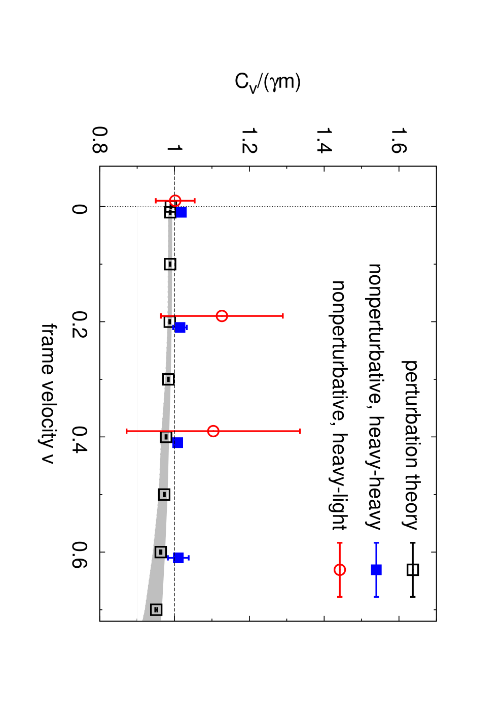
We write $C_{v}=\gamma m(1+\alpha_{s}\delta C_{v}+\dots)$ and the one-loop correction is given by

\displaystyle\delta C_{v}

\displaystyle=

\displaystyle\Omega_{2}-\Omega_{1}+\frac{\Omega_{0}}{\gamma m}\,.

(54)

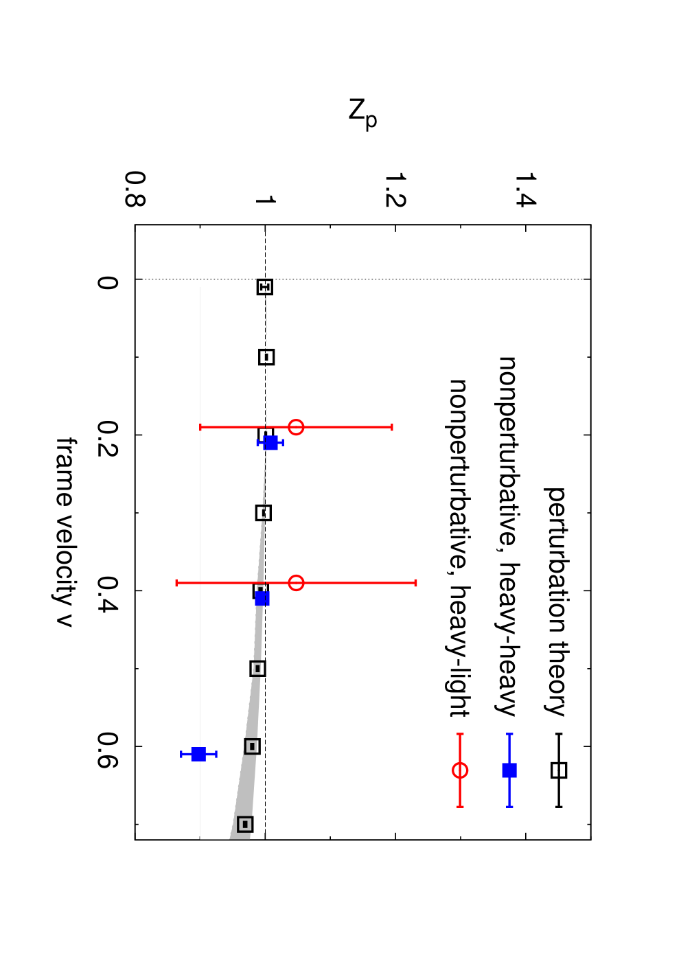
The shift $C_{v}$ and the renormalization of the external momentum can be obtained nonperturbatively by computing the energy $E_{v}({\boldsymbol{p}})$ of a heavy-heavy system which is up to lattice artifacts given by

E_{v}({\boldsymbol{p}})+2C_{v}=\sqrt{(2Z_{p}\gamma m{\boldsymbol{v}}+{\boldsymbol{p}})^{2}+M_{\operatorname{kin}}^{2}}\,.

A corresponding dispersion relation with $2C_{v}\mapsto C_{v}$ and $2Z_{p}\mapsto Z_{p}$ holds for heavy-light mesons containing only one heavy quark. We will compare values for the energy shift and the renormalization of the external momentum calculated in perturbation theory and nonperturbatively using the dispersion relation of heavy-heavy and heavy-light mesons in section VII.

V.3 Reparametrization invariance

One thing we expect from our results is that, because of lattice reparametrization invariance [33], the deviation of the momentum renormalization parameter $Z_{p}$ from its tree level result is much smaller than for other renormalization parameters. Reparametrization invariance is a symmetry that has been studied in the context of heavy quark effective theories [38, 39, 40]. This symmetry arises from the fact that the division of the full momentum $p$ into a “fixed” external part $m\>u$ and a “dynamic” residual part $k$ is not unique. We can always write $p=m\>u+k=m\>u^{\prime}+k^{\prime}$ where $k^{\prime}=k-m\epsilon$ , $u^{\prime}=u+\epsilon$ . The 4-velocities $u$ and $u^{\prime}$ have unit norm which implies the constraint on $\epsilon$ that $2\epsilon\cdot u+\epsilon\cdot\epsilon=0$ . It can be shown [39, 38] that this reparametrization of the full momentum is a symmetry of the effective heavy quark Lagrangian in the continuum.

Because mNRQCD is a non-relativistic formulation Lorentz symmetry is not manifest in the action. This is apparent from: the form of the FWT transformation (8); the field redefinition (section III.1.2) required to remove time derivatives in the Hamiltonian; the truncation of the action to a given order in $1/m$ ; and the non-relativistic field normalization (18). To adapt the discussion of reparametrization invariance to mNRQCD we study the ambiguity in division of the total 3-momentum, ${\boldsymbol{p}}=\gamma({\boldsymbol{v}})m\>{\boldsymbol{v}}+{\boldsymbol{k}}$ , keeping $|{\boldsymbol{v}}|$ fixed since it is a parameter in the Hamiltonian. We first consider a simple action with Hamiltonian

H_{0}=-i{\boldsymbol{v}}\cdot{\boldsymbol{D}}-\frac{{\boldsymbol{D}}^{2}}{2\gamma m}

(55)

omitting the term $({\boldsymbol{v}}\cdot{\boldsymbol{D}})^{2}/(2\gamma m)$ for the moment. This action is invariant under the transformation

\displaystyle v_{j}

\displaystyle\mapsto v_{j}+\epsilon_{j},

\displaystyle\psi

\displaystyle\mapsto e^{-i\gamma m{{\boldsymbol{\epsilon}}\cdot{\boldsymbol{x}}}}\psi

(56)

with $2{\boldsymbol{v}}\cdot{\boldsymbol{\epsilon}}+{\boldsymbol{\epsilon}}\cdot{\boldsymbol{\epsilon}}=0$ . This constraint ensures that $|{\boldsymbol{v}}^{\prime}|=|{\boldsymbol{v}}|$ . This is an exact symmetry which implies that the external momentum ${\boldsymbol{P}}_{0}=\gamma m{\boldsymbol{v}}$ is not renormalized as the relative coefficients of the two terms in (55) are fixed even after renormalization.

On the lattice, where we use the discretized Hamiltonian

\displaystyle H_{0}^{(\operatorname{lat})}

\displaystyle=

\displaystyle-i{\boldsymbol{v}}\cdot{\boldsymbol{\Delta}}^{\pm}-\frac{\Delta^{(2)}}{2\gamma am},

(57)

this symmetry is broken. Under (56) $H_{0}^{(\operatorname{lat})}$ transforms according to

\displaystyle H_{0}^{(\operatorname{lat})}

\displaystyle\mapsto

\displaystyle H_{0}^{(\operatorname{lat})}+\frac{1}{2}\gamma ma^{2}\sum_{j}\psi^{\dagger}v_{j}\epsilon_{j}\Delta_{j}^{+}\Delta_{j}^{-}\psi+{\mathcal{O}}(\epsilon^{2}).

If ${\boldsymbol{v}}$ is chosen along a lattice axis $v_{j}=v\delta_{j1}$ , say, then using the constraint on $\epsilon$ the factor $v_{j}\epsilon_{j}$ can be replaced by $-\frac{1}{2}|{\boldsymbol{\epsilon}}|^{2}\delta_{j1}$ which is small for small $\epsilon$ . We might therefore expect the breaking of reparametrization invariance by lattice artifacts in this case to be small. In the corresponding derivation with improved derivatives in $H_{0}^{(\operatorname{lat})}$ , we find that the lattice artifacts which break reparametrization invariance are of $\mathcal{O}(a^{4})$ .

Reparametrization invariance is broken even for the continuum theory unless the FWT transformation and the truncation of the action as a series in $1/m$ respect it. The field redefinition, designed to remove time derivatives in the Hamiltonian, must also be invariant under the reparametrization transformation. This will be satisfied only if the velocity and the covariant derivative appear in the combination [39, 38]

{\boldsymbol{v}}-\frac{i{\boldsymbol{D}}}{2\gamma m}\;.

(58)

This implies that terms of different order in $1/m$ are mixed by the reparametrization transformation and so any truncation of the action as a series in $1/m$ will break this invariance. It would be possible to include selected higher-order terms in $1/m$ by rewriting the action in terms of the combination (58) but in practice this is unnecessary since the approximate reparametrization invariance of the action is sufficient to restrict the renormalization $Z_{p}$ of the total quark momentum $P_{0}$ to be close to unity. It would also introduce extra terms of little significance in the non-relativistic expansion but which are expensive to evaluate computationally for the lattice theory. In any case discretization breaks the invariance as already discussed. We shall compute $Z_{p}$ both perturbatively and nonperturbatively.

The mixing is evident in our simple example above. It is easy to see that adding the term $({\boldsymbol{v}}\cdot{\boldsymbol{D}})^{2}/(2\gamma m)$ will break the invariance for non-zero frame velocities even in the continuum. This breaking is proportional to $v^{2}/(2\gamma m)$ , so it increases to reach a maximum at $v=\sqrt{2/3}\approx 0.8$ and then drops to zero due to the suppression by $1/\gamma$ . Numerically we find this behavior in our perturbative results for the simple action we discuss in Appendix E.1. The one-loop contribution to the external momentum renormalization vanishes for small $v$ , rises to a maximum at $v\approx 0.75$ and then drops again. At this velocity we also computed $\delta Z_{p}$ with the action (55) both with naïve and improved derivatives. We find that the use of improved derivatives reduces $\delta Z_{p}$ by roughly a factor 2.

Our numerical results (see Table 4, to be discussed in Sec. V.9) do indeed show that on the lattice $Z_{p}$ is very close to 1 for small frame velocities. For larger frame velocities the perturbative results show a deviation of $Z_{p}$ from the tree level value of at most 10% for practical choices of frame-velocity ${\boldsymbol{v}}$ .

V.4 Current construction

For calculations of hadronic matrix elements of weak interaction operators involving the heavy quark, the continuum QCD currents must be replaced by appropriate lattice currents. Let us, for example, consider the vector current

J^{\mu}(x)=\overline{q}(x)\hat{\gamma}^{\mu}\Psi(x)

where $q(x)$ is the Dirac field of the light quark and $\Psi(x)$ is the Dirac field of the heavy quark. At tree-level, it suffices to express $\Psi(x)$ via the Euclidean version of the field redefinition (21).

Recall that Eq. (7) contains a factor of $e^{-im{x^{\prime}}^{0}\hat{\gamma}^{0}}$ which removes the mass term from the Lagrangian. For a heavy quark, the lower two components of the non-relativistic field $\tilde{\Psi}^{\prime}(x^{\prime})$ in Eq. (7) are zero, so that $\hat{\gamma}^{0}\tilde{\Psi}^{\prime}(x^{\prime})=\tilde{\Psi}^{\prime}(x^{\prime})$ and hence $e^{-im{x^{\prime}}^{0}\hat{\gamma}^{0}}\tilde{\Psi}^{\prime}(x^{\prime})=e^{-im{x^{\prime}}^{0}}\tilde{\Psi}^{\prime}(x^{\prime})$ . Since the FWT transformation in this frame does not contain time derivatives, the factor $e^{-im{x^{\prime}}^{0}}$ can be moved to the left of $T^{\prime}_{\scriptscriptstyle\mathrm{FWT}}$ . (In the antiquark case, where the upper two components of $\tilde{\Psi}^{\prime}(x^{\prime})$ are zero, one has $e^{+im{x^{\prime}}^{0}}$ .)

Performing the other steps of the derivation in Section III again, it then follows that also the factor of $e^{-im\>u\cdot x\>\hat{\gamma}^{0}}$ in Eq. (21) can be moved to the left of $T_{\scriptscriptstyle\mathrm{FWT}}$ in the case where ${\xi_{v}}(x)=0$ . Thus, in correlation functions the factor $e^{-im\>u\cdot x\>\hat{\gamma}^{0}}$ trivially shifts energy and momentum and can be removed. We obtain

J^{\mu}(x)=\overline{q}(x)\hat{\gamma}^{\mu}\frac{1}{\sqrt{\gamma}}S(\Lambda)\>T_{\scriptscriptstyle\mathrm{FWT}}\>\>A_{\scriptscriptstyle D_{t}}\left(\begin{array}[]{c}{\psi_{v}}(x)\\ 0\end{array}\right).

For on-shell quantities, time derivatives in $T_{\scriptscriptstyle\mathrm{FWT}}$ and $A_{\scriptscriptstyle D_{t}}$ can be eliminated using the equations of motion, $D_{4}=i{\boldsymbol{v}}\cdot{\boldsymbol{D}}+\mathcal{O}(1/m)$ . The continuum derivatives are then replaced by lattice derivatives.

Beyond tree-level, additional lattice operators are required and matching coefficients must be introduced to correct for the different ultraviolet behavior of QCD and lattice mNRQCD. These matching coefficients can be computed perturbatively by comparing matrix elements between on-shell states in the continuum and lattice theories.

Note that the renormalization of the boost velocity also affects the spinorial boost matrix $S(\Lambda)$ . We have for bare quantities

\displaystyle S(\Lambda({\boldsymbol{v}}))

\displaystyle=

\displaystyle\frac{1}{\sqrt{2(1+\gamma)}}\left(\begin{array}[]{cc}1+\gamma&\gamma\>{\boldsymbol{\sigma}}\cdot{\boldsymbol{v}}\\ \gamma\>{\boldsymbol{\sigma}}\cdot{\boldsymbol{v}}&1+\gamma\end{array}\right)

and the renormalized matrix is obtained from this by an additional Lorentz boost,

\displaystyle S(\Lambda({\boldsymbol{v}}_{R}))

\displaystyle=

\displaystyle S(\Lambda(\delta{\boldsymbol{v}}))S(\Lambda({\boldsymbol{v}})).

(No Wigner rotation is needed here as only the magnitude of ${\boldsymbol{v}}$ is renormalized for ${\boldsymbol{v}}$ pointing in one of the lattice directions.) We find

\displaystyle S(\Lambda(\delta{\boldsymbol{v}}))

\displaystyle=

\displaystyle\left(\begin{array}[]{cc}1&\frac{1}{2}\delta{\boldsymbol{v}}\cdot{\boldsymbol{\sigma}}\\ \frac{1}{2}\delta{\boldsymbol{v}}\cdot{\boldsymbol{\sigma}}&1\end{array}\right)

with

\displaystyle\delta{\boldsymbol{v}}=\frac{{\boldsymbol{v}}_{R}-{\boldsymbol{v}}}{1-{\boldsymbol{v}}\cdot{\boldsymbol{v}}_{R}}

\displaystyle=

\displaystyle\alpha_{s}\delta Z_{v}\gamma^{2}{\boldsymbol{v}}.

We will not consider the current matching any further here; this will be discussed in another paper.

V.5 Lattice Perturbation Theory

Feynman rules for lattice actions are complicated and for all but the simplest cases an automated procedure is needed to obtain them. The formalism for this is due to Lüscher and Weisz [41]. This was extended by Nobes and Trottier [42] and Hart et al. [43, 44, 45] to include both relativistic and non-relativistic fermion actions such as HISQ [27] and, as used here, mNRQCD. In this paper we use the implementation of Hart et al. [43, 44, 45] to compute the one-loop self-energy $\Sigma(z)$ for various choices of mNRQCD Hamiltonian. The Feynman rules, vertices and propagators, are generated in machine-readable form using the Python program HiPPy and then used in the Fortran 95 code HPsrc to construct the diagrams and carry out the loop momentum integrations. The latter are done using vegas [46, 47] or, in the case of small lattices, by mode-summation. All perturbative results presented in this paper are obtained on an infinite lattice.

As more correction terms are added to the action, the number of terms in the perturbative expansion grows very fast, and so does computation time. We have used a version of vegas that has been adapted to parallel computing using MPI (Message Passing Interface).

The diagrams we evaluate to obtain the heavy quark self energy at one loop are shown in Fig. 3. The renormalization parameters require derivatives of the self energy. The derivatives of the Feynman rules were calculated exactly (rather than from small finite differences due to their associated errors and instabilities) and then automatically combined to form diagram derivatives using code based on the TaylUR package [48, 49] (which overloads arithmetic operations so as to respect Leibniz’s rule and the chain rule).

As an alternative to perturbation theory based on loop integrals, renormalized quantities may be measured by simulation in the weak coupling regime of the theory (i.e. at high $\beta$ ) [50, 51] on small lattices using ’t Hooft twisted boundary conditions [52, 41]. While not the subject of this paper, knowledge from analytic calculation of the one-loop corrections allows accurate fitting to extract the two-loop contributions. To implement twisted boundary conditions is straight-forward; it requires the spectrum of the momenta used to be appropriately modified and the vertices to carry a momentum-dependent phase rather than the usual color factor. We will discuss such calculations for mNRQCD in more detail in a forthcoming publication.

Figure 3: Diagrams to be evaluated: (

a

) rainbow diagram and (

b

) tadpole diagram. Numerical calculations show that contributions to the heavy quark self-energy from diagram (

b

) are approximately an order of magnitude bigger than those of diagram (

a

), demonstrating the crucial importance of tadpole improvements for any lattice-based perturbation theory calculation.

V.6 Contour shift

For a Euclidean lattice field theory the energy integral is nominally over the unit circle $|(z=e^{ik_{4}})|=1$ . However, the positions of the poles in the integrand are functions of the loop three-momentum and care must be taken that no pole crosses the contour: the contour must be distorted to avoid this happening. In particular, the heavy quark pole $z_{h}$ must remain inside the contour of integration in order to represent a forward-propagating heavy quark. This can be done by choosing $|z|=R,R>1$ where $R$ is chosen so that the contour is large enough to enclose $z_{h}$ and as distant from any pole as is possible to improve convergence of the integration. In Fig. 4 we show the position of the poles in the $z$ plane.

Figure 4: Position of poles in the complex

z

plane and integration contour (dashed circle). The two poles in the Wilson gluon action are

z_{\pm}

with

z_{+}z_{-}=1

whereas the heavy quark pole can be found at

z_{h}

. If

z_{h}>z_{-}

we shift the contour according to

z\mapsto Rz

with

R=\sqrt{z_{h}z_{+}}>1

This contour shift applies to the case of the rainbow diagram Fig. 3a but is not necessary for the tadpole graph in Fig. 3b as the poles in the gluon propagator corresponding to solutions moving forward/backward in time always come in pairs with $z_{+}z_{-}=1$ .

Finding the pole of the heavy quark propagator is straightforward as the Lagrangian only contains first order time derivatives [53]. Exact expressions for the position of the poles of the Wilson gluon action can also be derived. These and the extension to more complicated gauge actions are discussed in Appendix F. There we show that $|z_{-}^{(\operatorname{imp})}|<z_{-}<1<z_{+}<|z_{+}^{(\operatorname{imp})}|$ so that the contour shift derived for the Wilson action remains valid.

The additional contour shift which is necessary when formulating the theory in Euclidean space has been discussed in the literature [54, 55]. In Ref. [54], Aglietti et al. conclude that deriving Feynman rules for HQET in the Euclidean theory is problematic as a simple Wick rotation will generate unphysical solutions propagating backwards in time. However, in a subsequent paper [55], Aglietti extends the analysis and realizes that this is due to an incorrect rotation of the integration contour to Euclidean time. To avoid crossing the heavy quark pole at ${\boldsymbol{v}}\cdot{\boldsymbol{k}}$ it is necessary to rotate the contour around $-\Delta={\boldsymbol{v}}\cdot{\boldsymbol{k}}-\delta$ instead of the origin of the $k_{0}$ plane (see Fig. 5).

Figure 5: Wick rotation to Euclidean space for continuum HQET; the integration contour is shown as a dashed line. If the heavy quark pole at

\omega_{h}={\boldsymbol{v}}\cdot{\boldsymbol{k}}

lies to the left of the imaginary axis the contour has to be rotated around

-\Delta={\boldsymbol{v}}\cdot{\boldsymbol{k}}-\delta

. The gluon poles are denoted by

\omega_{\pm}

V.7 Treatment of infrared divergences

To deal with infrared divergences, we note that any lattice theory has the same infrared behavior as the equivalent continuum theory. Therefore we consider the diagrams of Fig. 3 where lattice Feynman rules have been replaced by equivalent continuum ones (noting that the two-gluon vertex is still present in continuum (m)NRQCD).

To analyze the infrared behavior of these diagrams we first perform the integration over the temporal component of the loop momentum as a contour integration, then look at the behavior of the remaining three-dimensional spatial integral for small loop momentum.

In the non-moving case ( $v=0$ ) this can conveniently be done in spherical polar coordinates; for the moving case we need to take into account the fact that the external velocity introduces a preferred direction. It is convenient to take the velocity to lie along the $x$ -axis, for instance.

After performing these calculations we see that the rainbow diagram Fig. 3a, as well as the tadpole diagram Fig. 3b and all derivatives of the tadpole diagram are infrared-finite; however the derivatives of the rainbow diagram behave for low momentum as $\sim\int\frac{dk}{k}$ and thus are logarithmically divergent. To regulate this divergence we introduce a small gluon mass $\lambda$ , which we may do because the rainbow diagram has Abelian color structure.

To find the infrared behavior of $\Omega_{1}$ , $\Omega_{2}$ , and $\Omega_{v}$ we perform the analytic calculations as detailed above, keeping track of all prefactors in the integration. After doing this, we obtain the infrared-divergent part of the derivative of the rainbow diagram:

-\frac{2}{3\pi}\log\lambda^{2}\;

(65)

which is the same as the IR divergence in continuum QCD, using the same regulator in both theories. In the matching coefficients between lattice mNRQCD and QCD the logarithmic dependence on the gluon mass will cancel out and we can set $\lambda=0$ at the end of the calculation.

We discuss three approaches to verify that this same divergence is present in the full lattice Feynman integrals.

V.7.1 Infrared subtraction function

The first approach is to construct a suitable subtraction function which can be integrated analytically and has the same infrared behavior as the lattice integrand. The subtracted lattice integral is then infrared-finite and the full result can be obtained by adding the analytical expression for the integral over the subtraction function. This method was also used in the current matching in Ref. [53].

Only the wavefunction renormalization (in Feynman gauge) is infrared divergent. All other renormalization constants are IR finite and can be computed directly. To construct a suitable subtraction function $f^{(\operatorname{sub})}$ for $\delta Z_{\psi}$ we start from the continuum integral in heavy quark effective theory. (Note that in principle $f^{(\operatorname{sub})}$ is arbitrary as long as it: agrees with the lattice integrand for small loop momenta $k$ ; is ultraviolet-finite in $d=4$ dimensions; and can be integrated analytically.)

The logarithmic UV divergence can be regulated without changing the infrared behavior by replacing

\frac{-i}{k_{0}-i{\boldsymbol{v}}\cdot{\boldsymbol{k}}}\mapsto\frac{2\gamma m}{(k+m\>u)^{2}+m^{2}}

(66)

in the (Euclidean) heavy quark propagator. The resulting integral (which is not restricted to the Brillouin zone) is readily evaluated and gives

\delta Z_{\psi}^{(\operatorname{sub})}=-\frac{2}{3\pi}\log\lambda^{2}+\mathcal{O}(\lambda/m).

(67)

This is exactly the logarithmic divergence found in (65). The subtracted integral $\delta\overline{Z}_{\psi}$ is evaluated numerically, defined through

$\displaystyle\delta Z_{\psi}$	$\displaystyle=$	$\displaystyle\int\frac{d^{4}k}{(2\pi)^{4}}\left(\theta_{\operatorname{BZ}}(k)f^{(\operatorname{lat})}(k)-f^{(\operatorname{sub})}(k)\right)$	(68)
		$\displaystyle\qquad+\;\;\delta Z_{\psi}^{(\operatorname{sub})}$
	$\displaystyle\equiv$	$\displaystyle\delta\overline{Z}_{\psi}-\frac{2}{3\pi}\log\lambda^{2}$

where $\theta_{\operatorname{BZ}}(k)$ is equal to 1 inside the Brillouin zone and vanishes for any $|k_{\mu}|>\pi/a$ .

While this method is easy to carry out for the case of the self-energy and vertex correction calculations, it becomes increasingly complicated when considering other calculations.

V.7.2 Direct calculation for different $\lambda$

The alternative, more generic way of isolating the IR divergent behavior is to run our integration for different values of $\lambda$ and then obtain the desired $\log\lambda^{2}$ behavior by numerically fitting a line through the points. For example, in Fig. 6 we show the wavefunction renormalization for $\lambda^{2}$ varying from $10^{-8}$ to $10^{-4}$ . Using a logarithmic scale on the horizontal axis we see a very clear linear behavior, which demonstrates the desired dependence on $\log\lambda^{2}$ . The fit to $C_{0}+C_{\scriptscriptstyle\mathrm{IR}}\log\lambda^{2}$ yields, with a $\chi^{2}$ per degree-of-freedom of $0.17$ , $C_{\scriptscriptstyle\mathrm{IR}}=-0.21220(14)\log\lambda^{2}$ , which agrees well with the analytic result $-2/(3\pi)=-0.2122\ldots$ .

The latter method can be applied to all kinds of calculations such as current matching calculations in mNRQCD. It can also be used when the expressions for the diagrams are so complex that obtaining the infrared counterterms analytically is not feasible. For the integrands considered here this method is not very resource- or time-intensive; even a preliminary investigation, with short integration runs and a small number of sampling points, can yield a plot with a very good fit, demonstrating clear $\log\lambda^{2}$ -dependence. For more complicated integrands, subtraction functions may still be necessary: the computer time required for vegas to sufficiently reduce the statistical errors as we lower $\lambda^{2}$ may well be prohibitive and, in addition, strong IR divergences can confuse the importance sampling used by vegas.

V.7.3 Twisted boundary conditions

Alternatively infrared divergences can be regulated by working on a lattice of finite size and using twisted periodic boundary conditions [52, 41] which provide a lower momentum cutoff. We have successfully implemented and tested this method but will not discuss it further here. More details will appear in a forthcoming publication.

V.8 Tadpole improvement

The tadpole improvement of the action was described in Section IV.2. We define $u_{0}$ to be the mean-link in Landau gauge. In perturbation theory $u_{0}=1-\alpha_{s}u_{0}^{(2)}+\ldots$ , with $u_{0}^{(2)}=0.750$ for the Symanzik-improved gluon action [56]. Mean-field corrections are then included as counterterms in the action. This leads to

\Omega_{j}\rightarrow\Omega_{j}+\Omega_{j}^{(\mathrm{tadpole})}

(69)

where $\Omega_{j}^{(\mathrm{tadpole})}$ are the resulting tadpole factors which we give explicitly below.

We choose the form of the time derivative in (26) so that the wavefunction renormalization is immune from mean-field corrections [14]. Thus we expect (and, indeed, find) that the tadpole improvement contributions to $\Omega_{0}$ and $\Omega_{1}$ are exactly equal and opposite. The approximate reparametrization invariance implies that the radiative corrections to $Z_{p}$ should be small, which suggests the tadpole corrections to $\Omega_{2}$ and to $\Omega_{v}$ should be very similar. Again, we find this to be the case.

The computation of the tadpole factors was checked in two separate calculations. We find

$\displaystyle\Omega^{(\mathrm{tadpole})}_{0}$	$\displaystyle=$	$\displaystyle-\Omega^{(\mathrm{tadpole})}_{1}$
	$\displaystyle=$	$\displaystyle u_{0}^{(2)}\bigg[1+7\frac{3-v^{2}}{6\gamma m}-\frac{3-6v^{2}+5v^{4}}{2\gamma^{3}m^{3}}$
		$\displaystyle\hskip 25.83325pt+\frac{1}{4n}\left(-v^{2}+\frac{-3+2v^{2}-v^{4}}{\gamma^{2}m^{2}}\right)$
		$\displaystyle\hskip 25.83325pt+\frac{1}{6n^{2}}\frac{-5v^{2}+3v^{4}}{\gamma m}-\frac{n+2}{16n^{3}}v^{4}\bigg],$
$\displaystyle\Omega^{(\mathrm{tadpole})}_{2}$	$\displaystyle=$	$\displaystyle-u_{0}^{(2)}\bigg[\frac{5}{3}+7\frac{3-v^{2}}{6\gamma m}+\frac{3-3v^{2}}{\gamma^{2}m^{2}}$
		$\displaystyle\hskip 30.1388pt-\frac{3-6v^{2}+5v^{4}}{2\gamma^{3}m^{3}}$
		$\displaystyle\hskip 30.1388pt+\;\;\frac{1}{4n}\left(-v^{2}+\frac{-3+2v^{2}-v^{4}}{\gamma^{2}m^{2}}\right)$
		$\displaystyle\hskip 30.1388pt+\frac{1}{6n^{2}}\left(2v^{2}+\frac{-5v^{2}+3v^{4}}{\gamma m}\right)$
		$\displaystyle\hskip 30.1388pt-\frac{n+2}{16n^{3}}v^{4}\bigg],$
$\displaystyle\Omega^{(\mathrm{tadpole})}_{v}$	$\displaystyle=$	$\displaystyle\Omega^{(\mathrm{tadpole})}_{2}\;-\;u_{0}^{(2)}\bigg[\frac{2v^{2}}{\gamma^{2}m^{2}}-\frac{v^{2}}{6n^{2}}\bigg]\,.$

For $v=0$ these expressions reduce to the ones obtained in [57]. Numerical values are given below in Table 3.

We give the corresponding expression for an alternative treatment of tadpole cancellation in Appendix D and list the tadpole improvement factors for other, simpler actions in Appendix E.

V.9 Perturbative results

In this section we present one-loop perturbative results for the renormalization of the mNRQCD propagator. Further results for a variety of simpler mNRQCD actions are given in Appendix E.

To obtain agreement with our numerical simulations, it is important that we use the Lüscher-Weisz gauge action [58, 59] which is used for the generation of MILC lattices [60]. For the heavy quark self energy at one-loop level, this action is equivalent to the tree-level Symanzik-improved gauge action

S_{G}=-\beta\sum_{\genfrac{}{}{0.0pt}{2}{x}{\mu<\nu}}\left(\frac{5}{3}P_{\mu\nu}(x)-\frac{1}{12}R_{\mu\mu\nu}(x)-\frac{1}{12}R_{\mu\nu\nu}(x)\right)\\ +\mathcal{O}(\alpha_{s})\;,

(70)

where $P$ , $R$ are $1\times 1$ and $2\times 1$ Wilson loops respectively. $\mathcal{O}(\alpha_{s})$ denotes possible radiative corrections and tadpole improvements of the action that only contribute at higher loop orders in the perturbative calculation of the heavy quark self energy.

For the squared gluon mass we choose a value of $\lambda^{2}=10^{-6}$ . The infrared-finite part of the wavefunction renormalization was extracted using a suitable subtraction function and we also checked that our results are indeed infrared-finite by varying $\lambda$ . The stability parameter is $n=2$ and for the heavy quark mass we use $m=2.8$ .

In Table 2 we list numerical results for $\Omega_{j}$ for a range of frame velocities before including mean-field corrections. We only give the finite parts of the $\Omega_{j}$ , the infrared divergence $-2/(3\pi)\log\lambda^{2}$ is not included in the results for $\Omega_{1}$ , $\Omega_{2}$ and $\Omega_{v}$ .

We give results for the tadpole improvement coefficients $\Omega^{(\mathrm{tadpole})}_{j}$ in Table 3 (see Table 16 in Appendix D for an alternative prescription). Finally we show the infrared-finite renormalization parameters, including mean-field corrections, in Table 4 and Fig. 7. In particular, note that the one-loop coefficient renormalizing the momentum is indeed small, as expected from the arguments presented in Sec. V.3.

$v$	$\Omega_{0}$	$\Omega_{1}$	$\Omega_{2}$	$\Omega_{v}$
$0.00$	$-2.36685(40)$	$2.03045(62)$	$3.0487(13)$	—
$0.01$	$-2.36672(39)$	$2.03042(62)$	$3.0470(13)$	$3.039(18)$
$0.10$	$-2.35534(40)$	$2.02033(62)$	$3.0276(13)$	$3.0192(24)$
$0.20$	$-2.32049(39)$	$1.98900(62)$	$2.9668(13)$	$2.9695(16)$
$0.30$	$-2.26205(38)$	$1.93675(62)$	$2.8646(14)$	$2.8857(14)$
$0.40$	$-2.17678(37)$	$1.86081(61)$	$2.7199(14)$	$2.7636(13)$
$0.50$	$-2.06318(35)$	$1.75964(61)$	$2.5330(15)$	$2.6023(12)$
$0.60$	$-1.91598(33)$	$1.62928(62)$	$2.3020(17)$	$2.4059(12)$
$0.70$	$-1.72666(31)$	$1.46150(63)$	$2.0220(20)$	$2.1623(11)$
$0.75$	$-1.61272(30)$	$1.36128(65)$	$1.8614(24)$	$2.0247(11)$
$0.80$	$-1.48224(28)$	$1.24847(69)$	$1.6828(29)$	$1.8794(11)$
$0.85$	$-1.33083(27)$	$1.12528(82)$	$1.4925(41)$	$1.7275(12)$
$0.90$	$-1.15125(25)$	$1.0118(11)$	$1.2930(68)$	$1.5972(15)$
$0.95$	$-0.92738(24)$	$1.0698(21)$	$1.236(19)$	$1.6559(25)$

Table 2: Infrared-finite part of

\Omega_{j}

for the full

\mathcal{O}(1/m^{2},v_{\operatorname{rel}}^{4})

action. The gluon action is Symanzik-improved with

\lambda^{2}=10^{-6}

and we use

m=2.8

n=2

. Mean-field corrections are not included and the errors shown are purely statistical from the vegas integration.

$v$	$\Omega^{(\mathrm{tadpole})}_{0}/u_{0}^{(2)}$	$\Omega^{(\mathrm{tadpole})}_{2}/u_{0}^{(2)}$	$\Omega^{(\mathrm{tadpole})}_{v}/u_{0}^{(2)}$
$0.00$	$2.13384$	$-3.18316$	—
$0.01$	$2.13375$	$-3.18300$	$-3.18302$
$0.10$	$2.12459$	$-3.16713$	$-3.16923$
$0.20$	$2.09650$	$-3.11915$	$-3.12728$
$0.30$	$2.04863$	$-3.03967$	$-3.05682$
$0.40$	$1.97963$	$-2.92963$	$-2.95725$
$0.50$	$1.88797$	$-2.79071$	$-2.82813$
$0.60$	$1.77221$	$-2.62561$	$-2.66939$
$0.70$	$1.63091$	$-2.43793$	$-2.48127$
$0.75$	$1.54999$	$-2.33677$	$-2.37612$
$0.80$	$1.46143$	$-2.23103$	$-2.26313$
$0.85$	$1.36379$	$-2.12013$	$-2.14118$
$0.90$	$1.25365$	$-2.00163$	$-2.00714$
$0.95$	$1.12074$	$-1.86625$	$-1.85110$

Table 3: Tadpole improvement corrections

\Omega^{(\mathrm{tadpole})}_{j}

for the full

\mathcal{O}(1/m^{2},v_{\operatorname{rel}}^{4})

action. The heavy quark mass is

m=2.8

and the stability parameter

n=2

. Note that

\Omega^{(\mathrm{tadpole})}_{1}=-\Omega^{(\mathrm{tadpole})}_{0}

$v$	$E_{0}$	$\delta\overline{Z}_{\psi}$	$\delta Z_{m}$	$\delta Z_{v}$	$\delta Z_{p}$	$\delta C_{v}$
$0.00$	$-0.76647(40)$	$-0.33639(48)$	$0.2313(12)$	—	—	$-0.0425(12)$
$0.01$	$-0.76641(39)$	$-0.33630(47)$	$0.2297(12)$	$-0.221(18)$	$-0.002(18)$	$-0.0441(12)$
$0.10$	$-0.76190(40)$	$-0.33501(47)$	$0.2275(12)$	$-0.2154(23)$	$0.0061(20)$	$-0.0454(12)$
$0.20$	$-0.74812(39)$	$-0.33149(48)$	$0.2194(12)$	$-0.2074(15)$	$0.0025(12)$	$-0.0510(12)$
$0.30$	$-0.72558(38)$	$-0.32530(48)$	$0.2037(12)$	$-0.1928(12)$	$-0.0087(10)$	$-0.0626(12)$
$0.40$	$-0.69206(37)$	$-0.31597(49)$	$0.1789(13)$	$-0.1696(11)$	$-0.02131(89)$	$-0.0799(13)$
$0.50$	$-0.64720(35)$	$-0.30354(50)$	$0.1421(13)$	$-0.1376(10)$	$-0.04175(86)$	$-0.1039(14)$
$0.60$	$-0.58682(33)$	$-0.28670(52)$	$0.0910(15)$	$-0.1037(10)$	$-0.06974(87)$	$-0.1350(16)$
$0.70$	$-0.50349(31)$	$-0.26516(55)$	$0.0158(17)$	$-0.06305(91)$	$-0.10943(92)$	$-0.1731(19)$
$0.75$	$-0.45023(30)$	$-0.25144(58)$	$-0.0337(19)$	$-0.04380(89)$	$-0.1394(10)$	$-0.1964(23)$
$0.80$	$-0.38616(28)$	$-0.23377(63)$	$-0.0901(24)$	$-0.02967(90)$	$-0.1746(11)$	$-0.2256(29)$
$0.85$	$-0.30798(27)$	$-0.20554(77)$	$-0.1502(32)$	$-0.01915(93)$	$-0.2235(11)$	$-0.2580(40)$
$0.90$	$-0.21101(25)$	$-0.1395(11)$	$-0.1933(51)$	$-0.0203(10)$	$-0.2966(13)$	$-0.3127(67)$
$0.95$	$-0.08682(24)$	$0.1425(21)$	$-0.038(14)$	$-0.0383(13)$	$-0.4374(16)$	$-0.402(18)$

Table 4: Heavy quark renormalization parameters for the full

\mathcal{O}(1/m^{2},v_{\operatorname{rel}}^{4})

action. The gluon action is Symanzik improved with

\lambda^{2}=10^{-6}

and we use

m=2.8

n=2

. All mean-field corrections are included and the results are infrared-finite. The errors shown are purely statistical from the vegas integration.

VI Numerical simulation results

In addition to the perturbative calculations described in the previous sections, we have performed a wide range of nonperturbative computations with the full mNRQCD action on unquenched gluon configurations. We have computed two-point correlation functions for various heavy-heavy and heavy-light mesons at different momenta and boost velocities. These allow the extraction of both energies and amplitudes. From the combination of simulation energies at different momenta, we have obtained nonperturbative results for the external momentum renormalization, the energy shift and the kinetic masses of the mesons. We have also examined the dependence of several energy splittings on the boost velocity. In addition to these spectral properties, we studied the behavior of decay constants.

The next section describes the simulations with heavy-heavy mesons and is followed by a section on heavy-light mesons. All results are given in lattice units.

Name	$n$	$L$	$S$	$J$	$P$	$C$	$\Gamma({\boldsymbol{r}})$
$\eta_{b}(1S)$	1	0	0	0	$-$	$+$	$\displaystyle\exp[-\|{\boldsymbol{r}}\|/r_{s}]\>\hat{\gamma}^{5}$
$\eta_{b}(2S)$	2	0	0	0	$-$	$+$	$\displaystyle\left[1-\|{\boldsymbol{r}}\|/(2r_{s})\right]\>\exp[-\|{\boldsymbol{r}}\|/(2r_{s})]\>\hat{\gamma}^{5}$
$\Upsilon(1S)$	1	0	1	1	$-$	$-$	$\displaystyle\exp[-\|{\boldsymbol{r}}\|/r_{s}]\>\hat{\gamma}^{j}$
$\Upsilon(2S)$	2	0	1	1	$-$	$-$	$\displaystyle\left[1-\|{\boldsymbol{r}}\|/(2r_{s})\right]\>\exp[-\|{\boldsymbol{r}}\|/(2r_{s})]\>\hat{\gamma}^{j}$
$\chi_{b1}(1P)$	1	1	1	1	$+$	$+$	$\displaystyle\>\exp[-\|{\boldsymbol{r}}\|/(2r_{s})]\>({\boldsymbol{r}}\times{\boldsymbol{\hat{\gamma}}})^{j}/r_{s}$

Table 5: Some (continuum) quantum numbers and smearing functions for the bottomonium system.

VI.1 Heavy-heavy mesons

VI.1.1 Methods

We begin by constructing “smeared” interpolating fields for quarkonium. To demonstrate the effect of the moving NRQCD field redefinition, we start the construction with the QCD fields $\overline{\Psi}$ , $\Psi$ . A meson with momentum ${\boldsymbol{p}}$ can be obtained from

O_{\Gamma}({\boldsymbol{p}},{\boldsymbol{\tau}})=\sum_{{\boldsymbol{x}}_{1},{\boldsymbol{x}}_{2}}\overline{\Psi}({\boldsymbol{x}}_{1},\tau)\Gamma({\boldsymbol{x}}_{1}-{\boldsymbol{x}}_{2})\Psi({\boldsymbol{x}}_{2},\tau)e^{-i{\boldsymbol{p}}\frac{{\boldsymbol{x}}_{1}+{\boldsymbol{x}}_{2}}{2}}

where $\Gamma({\boldsymbol{r}})$ is a Dirac-matrix-valued smearing function. We do not include gauge links in $\Gamma({\boldsymbol{r}})$ ; instead we fix the gauge configurations to Coulomb gauge. The (continuum) quantum numbers and corresponding functions $\Gamma({\boldsymbol{r}})$ used in the simulations are listed in Table 5.

We now express $\overline{\Psi}$ and $\Psi$ through the tree-level moving NRQCD field redefinition. To lowest order one has

	$\displaystyle\Psi(x)$	$\displaystyle=$	$\displaystyle\frac{1}{\sqrt{\gamma}}S(\Lambda)e^{-i\gamma m(-i\tau-{\boldsymbol{v}}\cdot{\boldsymbol{x}})\hat{\gamma}^{0}}\Psi_{v}(x),$
	$\displaystyle\overline{\Psi}(x)$	$\displaystyle=$	$\displaystyle\frac{1}{\sqrt{\gamma}}\>\overline{\Psi_{v}}(x)\>e^{i\gamma m(-i\tau-{\boldsymbol{v}}\cdot{\boldsymbol{x}})\hat{\gamma}^{0}}\>\>\overline{S(\Lambda)}.$

Let us, for example, consider the $\Upsilon$ states with polarization $j=1,2,3$ . We allow different smearing at source and sink, so that $\Gamma_{\rm sc}({\boldsymbol{r}})=\hat{\gamma}^{j}\>f_{\rm sc}({\boldsymbol{r}})$ and $\Gamma_{\rm sk}({\boldsymbol{r}})=\hat{\gamma}^{j}\>f_{\rm sk}({\boldsymbol{r}})$ . Using

\overline{S(\Lambda)}\>\hat{\gamma}^{j}\>S(\Lambda)=\Lambda^{j}_{\>\>\>\mu}\hat{\gamma}^{\mu},

(71)

we obtain

	$\displaystyle O_{\Gamma_{\rm sk}}({\boldsymbol{p}},\tau)O_{\Gamma_{\rm sc}}^{\dagger}({\boldsymbol{p}},\tau^{\prime})$	$\displaystyle=$	$\displaystyle\frac{1}{\gamma^{2}}e^{-2\gamma m(\tau-\tau^{\prime})}\sum_{{\boldsymbol{x}}_{1},{\boldsymbol{x}}_{2},{\boldsymbol{x}}^{\prime}_{1},{\boldsymbol{x}}^{\prime}_{2}}e^{-i{\boldsymbol{k}}\frac{{\boldsymbol{x}}_{1}+{\boldsymbol{x}}_{2}}{2}}f_{\rm sk}({\boldsymbol{x}}_{1}-{\boldsymbol{x}}_{2})e^{i{\boldsymbol{k}}\frac{{\boldsymbol{x}}^{\prime}_{1}+{\boldsymbol{x}}^{\prime}_{2}}{2}}f_{\rm sc}({\boldsymbol{x}}^{\prime}_{1}-{\boldsymbol{x}}^{\prime}_{2})$		(72)
			$\displaystyle\times\>\>\Lambda^{j}_{\>\>\>l}\Lambda^{j}_{\>\>\>m}\xi_{v}^{\dagger}({\boldsymbol{x}}_{1},\tau)\sigma^{l}\psi_{v}({\boldsymbol{x}}_{2},\tau)\psi_{v}^{\dagger}({\boldsymbol{x}}^{\prime}_{2},\tau^{\prime})\sigma^{m}\xi_{v}({\boldsymbol{x}}^{\prime}_{1},\tau^{\prime})+\>\>...$		(72)

(no summation over $j$ here) where

{\boldsymbol{k}}\equiv{\boldsymbol{p}}-2\gamma m{\boldsymbol{v}}.

(73)

The ellipsis in (72) denotes terms that do not contribute to the connected meson correlator for $\tau>\tau^{\prime}$ . The correlator is then given by

	$\displaystyle\langle O_{\Gamma_{\rm sk}}({\boldsymbol{p}},\tau)O_{\Gamma_{\rm sc}}^{\dagger}({\boldsymbol{p}},\tau^{\prime})\rangle$	$\displaystyle=$	$\displaystyle\frac{1}{N}\sum_{U}\frac{1}{\gamma^{2}}e^{-2\gamma m(\tau-\tau^{\prime})}\sum_{{\boldsymbol{x}}_{1},{\boldsymbol{x}}_{2},{\boldsymbol{x}}^{\prime}_{1},{\boldsymbol{x}}^{\prime}_{2}}e^{-i{\boldsymbol{k}}\frac{{\boldsymbol{x}}_{1}+{\boldsymbol{x}}_{2}}{2}}f_{\rm sk}({\boldsymbol{x}}_{1}-{\boldsymbol{x}}_{2})e^{i{\boldsymbol{k}}\frac{{\boldsymbol{x}}^{\prime}_{1}+{\boldsymbol{x}}^{\prime}_{2}}{2}}f_{\rm sc}({\boldsymbol{x}}^{\prime}_{1}-{\boldsymbol{x}}^{\prime}_{2})$		(74)
			$\displaystyle\times\>\>\Lambda^{j}_{\>\>\>l}\Lambda^{j}_{\>\>\>m}\mathrm{Tr}\left(\sigma^{l}\left[G_{\psi_{v}}^{U,{\boldsymbol{v}}}\left(({\boldsymbol{x}}_{2},\tau),({\boldsymbol{x}}^{\prime}_{2},\tau^{\prime})\right)\right]\sigma^{m}\left[G_{\psi_{v}}^{U,-{\boldsymbol{v}}}\left(({\boldsymbol{x}}_{1},\tau),({\boldsymbol{x}}^{\prime}_{1},\tau^{\prime})\right)\right]^{\dagger}\right),$		(74)

where we average over $N$ gauge configurations $U$ . The trace is over color and spin indices. We have also used equation () to express the antiquark green function $G_{\xi_{v}}^{U,{\boldsymbol{v}}}$ in terms of the quark green function $G_{\psi_{v}}^{U,-{\boldsymbol{v}}}$ with the opposite boost velocity.

The summations over all quark and antiquark source locations would render the lattice computation too expensive. Therefore, using translation invariance, we remove the summation over the antiquark source location ${\boldsymbol{x}}_{1}^{\prime}$ . Furthermore, we remove the factor of $e^{-2\gamma m(\tau-\tau^{\prime})}$ which corresponds to the tree-level energy shift. Hence, the quantity

	$\displaystyle C(\Gamma_{\rm sk},\Gamma_{\rm sc},{\boldsymbol{k}},\tau,\tau^{\prime})$	$\displaystyle=$	$\displaystyle\frac{1}{N}\sum_{U}\frac{1}{\gamma^{2}}\sum_{{\boldsymbol{x}}_{1},{\boldsymbol{x}}_{2}}e^{-i{\boldsymbol{k}}\frac{{\boldsymbol{x}}_{1}+{\boldsymbol{x}}_{2}}{2}}f_{\rm sk}({\boldsymbol{x}}_{1}-{\boldsymbol{x}}_{2})$
			$\displaystyle\times\Lambda^{j}_{\>\>\>l}\Lambda^{j}_{\>\>\>m}\mathrm{Tr}\left(\sigma^{l}\left[\tilde{G}_{\psi_{v}}^{U,{\boldsymbol{v}}}\left(({\boldsymbol{x}}_{2},\tau),({\boldsymbol{x}}^{\prime}_{1},\tau^{\prime})\right)\right]\sigma^{m}\left[G_{\psi_{v}}^{U,-{\boldsymbol{v}}}\left(({\boldsymbol{x}}_{1},\tau),({\boldsymbol{x}}^{\prime}_{1},\tau^{\prime})\right)\right]^{\dagger}\right)$

with

\tilde{G}_{\psi_{v}}^{U,{\boldsymbol{v}}}\left(({\boldsymbol{x}}_{2},\tau),({\boldsymbol{x}}^{\prime}_{1},\tau^{\prime})\right)=\sum_{{\boldsymbol{x}}^{\prime}_{2}}e^{i{\boldsymbol{k}}\frac{{\boldsymbol{x}}^{\prime}_{1}+{\boldsymbol{x}}^{\prime}_{2}}{2}}f_{\rm sc}({\boldsymbol{x}}^{\prime}_{1}-{\boldsymbol{x}}^{\prime}_{2})G_{\psi_{v}}^{U,{\boldsymbol{v}}}\left(({\boldsymbol{x}}_{2},\tau),({\boldsymbol{x}}^{\prime}_{2},\tau^{\prime})\right)

(75)

is computed on the lattice. The correlator (75) can be computed by using the function

e^{i{\boldsymbol{k}}\frac{{\boldsymbol{x}}^{\prime}_{1}+{\boldsymbol{x}}^{\prime}_{2}}{2}}f_{\rm sc}({\boldsymbol{x}}^{\prime}_{1}-{\boldsymbol{x}}^{\prime}_{2})

(76)

as the initial condition in the mNRQCD evolution equation (28). The momentum-dependent phase factor $\exp(i{\boldsymbol{k}}({\boldsymbol{x}}^{\prime}_{1}+{\boldsymbol{x}}^{\prime}_{2})/2)$ at the source improves the overlap with the momentum considered. However, since there is no sum over ${\boldsymbol{x}}^{\prime}_{1}$ , one may omit this factor to allow the calculation of correlators with different momenta from the same source.

In order to maintain the periodic boundary conditions, we set $f({\boldsymbol{r}})$ to zero for $|{\boldsymbol{r}}|>R_{s}$ with some cut-off radius $R_{s}$ smaller than half the length of the lattice.

On the finite volume lattice with periodic boundary conditions, the momentum ${\boldsymbol{k}}$ takes on discrete values, $k_{j}={2\pi\>n_{j}}/{L_{j}}$ where $L_{j}$ are the spatial extents of the lattice. However, the physical meson momentum ${\boldsymbol{p}}$ is expected to deviate from the tree-level relation (73), since mass and velocity are renormalized. One has

{\boldsymbol{p}}=2Z_{p}{\boldsymbol{P}}_{0}+{\boldsymbol{k}}\hskip 12.91663pt\mathrm{with}\hskip 12.91663pt{\boldsymbol{P}}_{0}=\gamma m{\boldsymbol{v}}.

(77)

We fit a matrix of correlators with different smearings at source and sink with the functional form

	$\displaystyle C(\Gamma_{\rm sk},\Gamma_{\rm sc},{\boldsymbol{k}},\tau,\tau^{\prime})\rightarrow A^{\rm sk}(A^{\rm sc})^{*}\bigg[e^{-E(\tau-\tau^{\prime})}\hskip 17.22217pt$

	$\displaystyle\hskip 17.22217pt+\sum_{n=1}^{n_{\rm exp}-1}B^{\rm sk}_{n}(B^{\rm sc}_{n})^{*}e^{-(E+\Delta E_{1}+...+\Delta E_{n})(\tau-\tau^{\prime})}\bigg]$		(78)

where $E$ is the energy of the meson ground state, $A^{\rm sc}$ and $A^{\rm sk}$ are the (real) ground state amplitudes of the operators at source and sink and $B^{\rm sc}_{n}$ , $B^{\rm sk}_{n}$ are (real) amplitudes for the $n$ -th excited state, relative to the ground state amplitude. We use the constrained fitting method described in [61], and increase the number of exponentials until the fit results and error estimates become independent of $n_{\rm exp}$ .

The full (physical) energy differs from the energy $E=E_{v}({\boldsymbol{k}})$ obtained from the fit by twice the mNRQCD energy shift,

E_{\rm phys}=E_{v}({\boldsymbol{k}})+2C_{v}.

(79)

In perturbation theory, one has

C_{v}=Z_{m}Z_{\gamma}\gamma m+E_{0}.

(80)

Given expression (77) for the full (physical) momentum, we expect that, up to lattice artifacts,

	$\displaystyle E_{\rm phys}$	$\displaystyle=$	$\displaystyle\sqrt{{\boldsymbol{p}}^{2}+M_{\mathrm{kin}}^{2}}$		(81)
		$\displaystyle=$	$\displaystyle\sqrt{(2Z_{p}{\boldsymbol{P}}_{0}+{\boldsymbol{k}})^{2}+M_{\mathrm{kin}}^{2}}$		(81)

where $M_{\mathrm{kin}}$ is the kinetic mass of the meson.

Using (81), we can obtain nonperturbative results for $C_{v}$ , $Z_{p}$ and $M_{\rm kin}$ from the energies at various non-zero lattice momenta in combination with the energy at ${\boldsymbol{k}}=0$ :

$\displaystyle C_{v}$	$\displaystyle\!=\!$	$\displaystyle\frac{1}{2}\frac{{\boldsymbol{k}}^{2}_{\perp}-\left(E^{2}_{v}({\boldsymbol{k}}_{\perp})-E^{2}_{v}(0)\right)}{2(E_{v}({\boldsymbol{k}}_{\perp})-E_{v}(0))},$	(82)
$\displaystyle Z_{p}$	$\displaystyle\!=\!$	$\displaystyle\frac{E^{2}_{v}({\boldsymbol{k}}_{\parallel})\!-\!E^{2}_{v}(-{\boldsymbol{k}}_{\parallel})\!+\!4C_{v}(E_{v}({\boldsymbol{k}}_{\parallel})\!-\!E_{v}(-{\boldsymbol{k}}_{\parallel}))}{4{\boldsymbol{k}}_{\parallel}\cdot 2{\boldsymbol{P_{0}}}},$
$\displaystyle M_{\mathrm{kin}}$	$\displaystyle\!=\!$	$\displaystyle\sqrt{(E_{v}({\boldsymbol{k}})+2C_{v})^{2}-(2Z_{p}{\boldsymbol{P_{0}}}+{\boldsymbol{k}})^{2}}.$	(84)

Here, ${\boldsymbol{k}}_{\parallel}$ is parallel to ${\boldsymbol{v}}$ , and ${\boldsymbol{k}}_{\perp}$ is perpendicular to ${\boldsymbol{v}}$ . In order to fully take into account correlations in the energies at different momenta, we use the bootstrap method, performing fits on 500 bootstrap ensembles and computing the final quantity 500 times. The errors are then estimated as the 68% width of the resulting distribution.

Ultimately we will be interested in semileptonic $B$ decay matrix elements. As a simpler test we first study the decay of the $\eta_{b}(1S)$ meson via a fictitious axial vector current. The corresponding decay constant is defined by

\langle 0|\mathsf{J}_{5}^{\mu}(0)|\eta_{b}(1S),{\boldsymbol{p}}\rangle=if\>p^{\mu}.

(85)

Here, $\mathsf{J}_{5}^{\mu}$ is the mNRQCD field operator associated with the axial current

J_{5}^{\mu}(x)=\overline{\Psi}(x)\>\hat{\gamma}^{5}\hat{\gamma}^{\mu}\>\Psi(x).

(86)

For simplicity, we have only considered the temporal component and, as above, used only the leading-order tree-level mNRQCD field redefinition to construct the lattice current. To extract the amplitude, we compute $2\times 2$ matrix correlators with the local smearing function

\Gamma({\boldsymbol{r}})=\delta({\boldsymbol{r}})\>\hat{\gamma}^{5}\hat{\gamma}^{0}

(87)

for the temporal axial current, and the $\eta_{b}(1S)$ smearing function from Table 5. The product of the ground state amplitudes in (78) is given by

	$\displaystyle A^{\rm sk}(A^{\rm sc})^{*}$	$\displaystyle=$	$\displaystyle\frac{1}{2E_{\rm phys}}\langle\eta_{b}(1S),{\boldsymbol{p}}\|\mathsf{O}_{\Gamma_{\rm sk}}(0)\|0\rangle$		(88)
			$\displaystyle\hskip 13.77771pt\times\>\>\>\>\>\>\langle 0\|\mathsf{O}_{\Gamma_{\rm sc}}(0)\|\eta_{b}(1S),{\boldsymbol{p}}\rangle,$		(88)

as can be seen from the spectral decomposition of the two-point correlator. Using (85) with $p^{0}=E_{\rm phys}$ , (79) and (88), we obtain

f=A\>\sqrt{\frac{2}{E_{v}({\boldsymbol{k}})+2C_{v}}}

(89)

where $A=A^{\rm sk/sc}$ is the amplitude from the fit corresponding to $\Gamma_{\rm sk/sc}=\delta({\boldsymbol{r}})\>\hat{\gamma}^{5}\hat{\gamma}^{0}$ .

VI.1.2 Lattice parameters

The computations were performed using 400 MILC gauge configurations (fixed to Coulomb gauge) of size $20^{3}\times 64$ with 2+1 flavors of rooted staggered light quarks, at $\beta=6.76$ [60]. The light quark masses were $m_{u}=m_{d}=0.007$ and $m_{s}=0.05$ (in the MILC convention for lattice masses). The Landau gauge mean link, used in the mNRQCD action, was $u_{0}=0.836$ . The inverse lattice spacing of these “coarse” MILC configurations is known to be approximately 1.6 GeV [62].

Heavy quark propagators were computed using full mNRQCD lattice action described in section IV and used in the perturbative calculation. The bare heavy quark mass was set to $m=2.8$ , which gave the correct $\Upsilon$ kinetic masses using non-moving NRQCD [62]. The boost velocity was always pointing in the $x$ -direction, ${\boldsymbol{v}}=(v,0,0)$ . The stability parameter was set to $n=2$ .

In order to increase statistics, between 16 and 120 correlators with different origins $({\boldsymbol{x}}^{\prime}_{1},\tau^{\prime})$ spread over the lattice were calculated and averaged over on each gauge configuration. These origins were also shifted randomly to reduce autocorrelations. The smearing parameter $r_{s}$ was set to 1 for the S wave states and 0.5 for the P wave states.

VI.1.3 Results

$\|{\boldsymbol{v}}\|$	$Z_{p}$	$M_{\textrm{kin}}$	$C_{v}/(\gamma m)$	$Z_{p}$	$M_{\textrm{kin}}$	$C_{v}/(\gamma m)$
	$\|{\boldsymbol{k}}_{\perp}\|=\|{\boldsymbol{k}}_{\parallel}\|=2\pi/L$			$\|{\boldsymbol{k}}_{\perp}\|=\|{\boldsymbol{k}}_{\parallel}\|=4\pi/L$
$0$	—	$5.974(48)$	$1.0182(86)$	—	$5.979(37)$	$1.0190(65)$
$0.2$	$1.008(19)$	$5.95(10)$	$1.015(18)$	$1.009(12)$	$5.969(62)$	$1.017(11)$
$0.4$	$0.9953(78)$	$5.931(44)$	$1.0084(77)$	$0.9830(65)$	$5.954(40)$	$1.0101(70)$
$0.6$	$0.898(27)$	$6.22(18)$	$1.010(28)$	$0.843(27)$	$6.37(15)$	$1.011(21)$

Table 6: Nonperturbative results (using the

\eta_{b}(1S)

) for

M_{\mathrm{kin}}

Z_{p}

C_{v}

Results for the $\eta_{b}(1S)$ kinetic mass $M_{\mathrm{kin}}$ and the renormalization parameters $Z_{p}$ , $C_{v}$ are shown in Table 6. The energies were obtained from 6-exponential fits to $2\times 2$ matrix correlators with the $\eta_{b}(1S)$ smearing and the local axial current. For the calculation of $C_{v}$ using (82), we averaged the results over the 4 different perpendicular lattice momenta

{\boldsymbol{k}}_{\perp}\in\left\{\frac{2\pi}{L}(0,\pm 1,0),\frac{2\pi}{L}(0,0,\pm 1)\right\}.

(90)

The momentum parallel to the boost velocity in () was chosen to be ${\boldsymbol{k}}_{\parallel}=\frac{2\pi}{L}(1,0,0)$ , and in (84), for the measurement of $M_{\mathrm{kin}}$ , we use ${\boldsymbol{k}}=0$ .

Because the lattice is of finite extent, $L=20$ in our test case, the estimates for $C_{v}$ and $Z_{p}$ will be affected by the choice of momenta in (82) and () since the formulae are accurate only in the limit that the momenta are infinitesimal. Note that the uncertainty due to using non-infinitesimal momenta will decrease for larger lattices for which smaller momenta are available.

To estimate the size of the resulting systematic error we also performed the calculations with the larger momenta

{\boldsymbol{k}}_{\perp}\in\left\{\frac{2\pi}{L}(0,\pm 2,0),\frac{2\pi}{L}(0,0,\pm 2)\right\},{\boldsymbol{k}}_{\parallel}=\frac{2\pi}{L}(2,0,0).

(91)

For $C_{v}$ , the results from $|{\boldsymbol{k}}_{\perp}|=2\pi/L$ agree with those obtained from $|{\boldsymbol{k}}_{\perp}|=4\pi/L$ within statistical errors, indicating that the systematic error is small and does not increase significantly when increasing the momentum perpendicular to ${\boldsymbol{v}}$ in the measurement. For the measurement of $Z_{p}$ at $|{\boldsymbol{v}}|=0.6$ we find a 6% ( $2\sigma$ ) change in $Z_{p}$ when going from $|{\boldsymbol{k}}_{\parallel}|=2\pi/L$ to $|{\boldsymbol{k}}_{\parallel}|=4\pi/L$ . At $|{\boldsymbol{v}}|=0.4$ and smaller boost velocities the results are equal within statistical errors. For the kinetic mass, which depends on both $C_{v}$ and $Z_{p}$ , we again find agreement within statistical errors between the results from the two different momenta for all boost velocities considered. At small velocities, we find that both $Z_{p}$ and $C_{v}/(\gamma m)$ are close to their tree-level value of 1, demonstrating that renormalizations are indeed small.

We also obtained the amplitude for the axial current and extracted the pseudoscalar decay constant from the same $2\times 2$ matrix fits using (89). For the energy shift $C_{v}$ in (89) we used the result from $|{\boldsymbol{k}}_{\perp}|=2\pi/L$ . The meson momentum is given by ${\boldsymbol{p}}=2Z_{p}\gamma m{\boldsymbol{v}}+{\boldsymbol{k}}$ . In the following we compare two methods of reaching large $|{\boldsymbol{p}}|$ . First, at ${\boldsymbol{v}}=0$ , i.e. with standard NRQCD, we computed the decay constant at large non-zero lattice momentum ${\boldsymbol{k}}$ ; the results are shown in Table 7. Second, we computed the decay constant with ${\boldsymbol{k}}=0$ and three different boost velocities ${\boldsymbol{v}}$ ; the results are shown in Table 8. In this case the uncertainty in $Z_{p}$ leads to an uncertainty in the meson momentum.

$\|{\boldsymbol{p}}\|L/(2\pi)$	$\|{\boldsymbol{p}}\|$	$f$
$0$	$0$	$0.4724(23)$
$1$	$0.31416$	$0.4731(23)$
$2$	$0.62832$	$0.4755(24)$
$3$	$0.94248$	$0.4772(43)$
$4$	$1.25664$	$0.4835(77)$
$5$	$1.57080$	$0.4971(78)$
$6$	$1.88496$	$0.5209(46)$
$7$	$2.19911$	$0.5527(44)$
$8$	$2.51327$	$0.6006(45)$
$9$	$2.82743$	$0.6740(49)$
$10$	$3.14159$	$0.715(29)$

Table 7:

\eta_{b}(1S)

decay constant with standard NRQCD (i.e.

{\boldsymbol{v}}=0

) computed with several values of meson momentum

|{\boldsymbol{p}}|

by varying

|{\boldsymbol{k}}|

$\|{\boldsymbol{v}}\|$	$\|{\boldsymbol{p}}\|$	$f$
$0$	$0$	$0.4724(23)$
$0.2$	$1.152(22)$	$0.4739(38)$
$0.4$	$2.433(19)$	$0.4810(36)$
$0.6$	$3.77(11)$	$0.499(11)$

Table 8:

\eta_{b}(1S)

decay constant with mNRQCD at

{\boldsymbol{k}}=0

computed with several values of meson momentum

|{\boldsymbol{p}}|

by varying

|{\boldsymbol{v}}|

A plot of the decay constant against the total momentum (with $Z_{p}$ from () with $|{\boldsymbol{k}}_{\parallel}|=2\pi/L$ ) for the two methods is shown in Fig. 8. The decay constant is a Lorentz scalar and should be independent of the momentum. However, with NRQCD we see large deviations due to both relativistic and discretization errors. With moving NRQCD the deviation is very small, giving evidence that the formalism works very well. Small deviations are still expected here, since only the leading-order current was used; i.e. $T_{\scriptscriptstyle\mathrm{FWT}}$ and $A_{\scriptscriptstyle D_{t}}$ were set to unity in (21) for this calculation.

Figure 8: Heavy-heavy decay constant in NRQCD and mNRQCD for different values of the meson’s momentum,

|{\boldsymbol{p}}|/(2\pi/L)=0\dots 10

(NRQCD) and

{\boldsymbol{p}}=Z_{p}\>2\gamma m{\boldsymbol{v}}

for

|{\boldsymbol{v}}|=0.2,0.4,0.6

(mNRQCD). The horizontal line indicates the value at

{\boldsymbol{p}}=0

Next, we studied the velocity-dependence of various energy splittings between the bottomonium states listed in Table 5. For the $\Upsilon$ and $\eta_{b}$ states, we used 6-exponential $2\times 2$ matrix fits with the $1S$ and $2S$ smearings; for the $\chi_{b1}$ states a 6-exponential single-correlator fit with the $1P$ smearing at both source and sink was used. The results for the $\Upsilon(2S)-\Upsilon(1S)$ , $\chi_{b1}(1P)-\Upsilon(1S)$ and $\Upsilon(1S)-\eta_{b}(1S)$ splittings are listed in Tables 9, 10 and 11, respectively.

$\|{\boldsymbol{v}}\|$	$\Delta E_{v}(0)$	$\displaystyle\frac{\Delta E_{v}(0)}{\Delta E_{0}(0)}$
$0.0$	$0.3334(68)$	1
$0.2$	$0.329(10)$	$0.986(37)$
$0.4$	$0.320(15)$	$0.958(48)$
$0.6$	$0.20(11)$	$0.59(33)$

Table 9:

\Upsilon(2S)-\Upsilon(1S)

energy splitting as a function of the boost velocity.

$\|{\boldsymbol{v}}\|$	$\Delta E_{v}(0)$	$\displaystyle\frac{\Delta E_{v}(0)}{\Delta E_{0}(0)}$
$0.0$	$0.2703(89)$	1
$0.2$	$0.264(12)$	$0.976(56)$
$0.4$	$0.270(23)$	$0.998(91)$
$0.6$	$0.227(57)$	$0.84(21)$

Table 10:

\chi_{b1}(1P)-\Upsilon(1S)

energy splitting as a function of the boost velocity.

$\|{\boldsymbol{v}}\|$	$\Delta E_{v}(0)$	$\displaystyle\frac{\Delta E_{v}(0)}{\Delta E_{0}(0)}$
$0.0$	$0.031469(98)$	1
$0.2$	$0.03039(20)$	$0.9656(71)$
$0.4$	$0.02837(85)$	$0.901(27)$
$0.6$	$0.0281(28)$	$0.894(88)$

Table 11:

\Upsilon(1S)-\eta_{b}(1S)

energy splitting as a function of the boost velocity.

$\|{\boldsymbol{v}}\|$	$\Delta E_{v}(0)\|_{1}$	$\Delta E_{v}(0)\|_{2}$	$\Delta E_{v}(0)\|_{3}$
$0$	$-0.000009(63)$	$-0.000039(68)$	$0.000053(73)$
$0.2$	$-0.00012(26)$	$-0.00005(28)$	$0.00017(30)$
$0.4$	$-0.00046(56)$	$0.00055(62)$	$-0.00010(57)$
$0.6$	$-0.0176(96)$	$0.0107(62)$	$0.0069(75)$

Table 12: Dependence of the

\Upsilon(1S)

energy on the polarization direction.

\Delta E_{v}(0)|_{j}

is the difference between

E_{v}(0)|_{j}

and the polarization-averaged energy.

Note that the energy splittings are not Lorentz scalars. Using (81), we expect that the splitting between two states $A$ and $B$ at zero lattice momentum is given by

	$\displaystyle E^{A}_{\boldsymbol{v}}(0)-E^{B}_{\boldsymbol{v}}(0)$	$\displaystyle=$	$\displaystyle\sqrt{(2Z_{p}\gamma m{\boldsymbol{v}})^{2}+(M^{A}_{\mathrm{kin}})^{2}}$
			$\displaystyle-\sqrt{(2Z_{p}\gamma m{\boldsymbol{v}})^{2}+(M^{B}_{\mathrm{kin}})^{2}}.$

If we set $Z_{p}=1$ and expand the splitting at velocity ${\boldsymbol{v}}$ relative to ${\boldsymbol{v}}=0$ in powers of the boost velocity, we obtain

\frac{E^{A}_{\boldsymbol{v}}(0)-E^{B}_{\boldsymbol{v}}(0)}{E^{A}_{0}(0)-E^{B}_{0}(0)}=1-\underbrace{\left(\frac{2m^{2}}{M^{A}_{\mathrm{kin}}\>M^{B}_{\mathrm{kin}}}\right)}_{\approx 0.5}\>{\boldsymbol{v}}^{2}+\mathcal{O}({\boldsymbol{v}}^{4}),

that is, we expect a quadratic decrease like $1-0.5|{\boldsymbol{v}}|^{2}$ . The numerical results, shown in Fig. 9, are consistent with this estimate as desired.

Finally, for the $\Upsilon(1S)$ meson, we studied the dependence of the energy on the polarization direction. If moving NRQCD works well, then there should be no difference for polarizations parallel and perpendicular to the boost velocity. In Table 12 we show the difference between the energy with definite polarization direction, $E_{v}(0)|_{j}$ and the polarization-direction-averaged energy $\frac{1}{3}(E_{v}(0)|_{1}+E_{v}(0)|_{2}+E_{v}(0)|_{3})$ . No significant dependence on the polarization direction can be seen (except maybe at $v=0.6$ , where a $1.8\sigma$ deviation in the energies was found).

VI.2 Heavy-light mesons

VI.2.1 Methods

Starting with the standard Dirac fields, we construct interpolating fields for the $B_{s}$ and $B_{s}^{*}$ mesons with momentum ${\boldsymbol{p}}$ from

O_{\Gamma}({\boldsymbol{p}},{\boldsymbol{\tau}})=\sum_{{\boldsymbol{x}},{\boldsymbol{y}}}\overline{\Psi}_{l}({\boldsymbol{x}},\tau)\Gamma({\boldsymbol{x}}-{\boldsymbol{y}})\Psi_{H}({\boldsymbol{y}},\tau)e^{-i{\boldsymbol{p}}\cdot{\boldsymbol{y}}}\;,

(92)

where $\Psi_{l}$ is the Dirac spinor for the valence strange quark and $\Psi_{H}$ is the Dirac spinor for the $b$ quark. We use $\Gamma({\boldsymbol{r}})=\hat{\gamma}^{5}\>f({\boldsymbol{r}})$ for the $B_{s}$ pseudoscalar meson, $\Gamma({\boldsymbol{r}})=\hat{\gamma}^{j}\>f({\boldsymbol{r}})$ with $j=1,2,3$ for the $B^{*}_{s}$ vector meson and $\Gamma({\boldsymbol{r}})=\hat{\gamma}^{5}\hat{\gamma}^{0}\>f({\boldsymbol{r}})$ for the computation of the decay constant $f_{B_{s}}$ . We compute $2\times 2$ matrix correlators with Gaussian and local smearing, $f({\boldsymbol{r}})=e^{-|{\boldsymbol{r}}|^{2}/r_{s}^{2}},\>\>\delta({\boldsymbol{r}})$ .

In terms of the standard Dirac propagators, the two-point function reads

	$\displaystyle\langle O_{\Gamma_{\rm sk}}({\boldsymbol{p}},\tau)O_{\Gamma_{\rm sc}}^{\dagger}({\boldsymbol{p}},\tau^{\prime})\rangle=\frac{1}{N}\sum_{U}\sum_{{\boldsymbol{x}},{\boldsymbol{y}},{\boldsymbol{x^{\prime}}},{\boldsymbol{y^{\prime}}}}$
	$\displaystyle\times\>\>\mathrm{Tr}\left[\>\Gamma_{\rm sk}({\boldsymbol{x}}-{\boldsymbol{y}})\>G_{l}\left(x^{\prime},\>x\right)\>\Gamma_{\rm sc}^{\dagger}({\boldsymbol{x^{\prime}}}-{\boldsymbol{y^{\prime}}})\>G_{H}\left(y,\>y^{\prime}\right)\>\right]$
	$\displaystyle\times\>\>e^{-i{\boldsymbol{p}}\cdot{\boldsymbol{y}}}e^{i{\boldsymbol{p}}\cdot{\boldsymbol{y^{\prime}}}}\;,$		(93)

with $x=({\boldsymbol{x}},\tau)$ , $y=({\boldsymbol{y}},\tau)$ , $x^{\prime}=({\boldsymbol{x^{\prime}}},\tau^{\prime})$ , $y^{\prime}=({\boldsymbol{y^{\prime}}},\tau^{\prime})$ . For $\tau>\tau^{\prime}$ , the tree-level leading-order mNRQCD field redefinition (21) leads to the following expression for the $b$ propagator:

	$\displaystyle G_{H}\left(y,\>y^{\prime}\right)$	$\displaystyle=$	$\displaystyle\frac{1}{\gamma}e^{-\gamma m(\tau-\tau^{\prime})+i\gamma m{\boldsymbol{v}}\cdot({\boldsymbol{y}}-{\boldsymbol{y^{\prime}}})}$
			$\displaystyle\times\>\>S(\Lambda)\left(\begin{array}[]{cc}G_{\psi_{v}}(y,\>y^{\prime})&0\\ 0&0\end{array}\right)\overline{S}(\Lambda).$

For the light quark, we use the ASQTAD staggered fermion action [34]. The 4-component naïve light quark propagator can be obtained from the 1-component staggered propagator $G_{\chi}(x^{\prime},x)$ via

G_{l}(x^{\prime},x)=\>G_{\chi}(x^{\prime},x)\otimes\Omega(x^{\prime})\Omega^{\dagger}(x)

(95)

with

\Omega(x)=(\hat{\gamma}^{0})^{x_{4}}(-i\hat{\gamma}^{1})^{x_{1}}(-i\hat{\gamma}^{2})^{x_{2}}(-i\hat{\gamma}^{3})^{x_{3}}.

(96)

(Recall our convention for the Dirac matrices is as given in Appendix A.) We also employ $\hat{\gamma}^{5}$ -hermiticity

G_{l}(x^{\prime},x)=\hat{\gamma}^{5}G_{l}^{\dagger}(x,x^{\prime})\hat{\gamma}^{5},

(97)

to interchange the points $x$ and $x^{\prime}$ for the light quark propagator. As before, we remove the factor of $e^{-\gamma m(\tau-\tau^{\prime})}$ and the summation over ${\boldsymbol{x^{\prime}}}$ .

In the case where $\Gamma_{\rm sk}$ and $\Gamma_{\rm sc}$ contain the same Dirac matrix, we arrive at the following expression:

		$\displaystyle C(\Gamma_{\rm sk},\Gamma_{\rm sc},{\boldsymbol{k}},\tau,\tau^{\prime})=\frac{1}{N}\!\sum_{U}\!\frac{1}{\gamma}\sum_{{\boldsymbol{x}},{\boldsymbol{y}}}f_{\rm sk}({\boldsymbol{x}}\!-\!{\boldsymbol{y}})e^{-i{\boldsymbol{k}}\cdot{\boldsymbol{y}}}\eta(x,x^{\prime})$
		$\displaystyle\times\mathrm{Tr}\left[G^{\dagger}_{\chi}(x,x^{\prime})\>\overline{S}(\Lambda)\Omega(x^{\prime})\Omega^{\dagger}(x)S(\Lambda)\!\left(\!\!\begin{array}[]{cc}\tilde{G}_{\psi_{v}}(y,\>x^{\prime})&0\\ 0&0\end{array}\!\!\right)\right]$

with ${\boldsymbol{k}}\equiv{\boldsymbol{p}}-\gamma m{\boldsymbol{v}}$ and

\tilde{G}_{\psi_{v}}(y,\>x^{\prime})=\sum_{{\boldsymbol{y^{\prime}}}}f({\boldsymbol{x^{\prime}}}-{\boldsymbol{y^{\prime}}})e^{i{\boldsymbol{k}}\cdot{\boldsymbol{y^{\prime}}}}G_{\psi_{v}}(y,y^{\prime}).

The phase factor $\eta(x,x^{\prime})$ in () depends on the Dirac matrix in $\Gamma_{\rm sk}$ and $\Gamma_{\rm sc}$ . It is given by

\eta(x,x^{\prime})=\left\{\begin{array}[]{ll}1&\mathrm{for}\>\>\hat{\gamma}^{5},\\ (-1)^{x^{\prime}_{j}-x_{j}}&\mathrm{for}\>\>\hat{\gamma}^{j},\\ (-1)^{\sum_{j}(x_{j}+x^{\prime}_{j})}&\mathrm{for}\>\>\hat{\gamma}^{5}\hat{\gamma}^{0}.\end{array}\right.

As before, we set $f({\boldsymbol{r}})$ to zero for $|{\boldsymbol{r}}|>R_{s}$ with some cut-off radius $R_{s}$ smaller than half the length of the lattice.

The staggered/naïve light quark action used here suffers from the doubling problem. As shown in [34], the spatial doublers do not contribute to the correlators. However, the temporal doubler leads to a coupling to additional opposite parity states, which manifest themselves as oscillating exponentials in the correlators. We therefore fit the heavy-light correlators to

	$\displaystyle C(\Gamma_{\rm sk},\Gamma_{\rm sc},{\boldsymbol{k}},\tau,\tau^{\prime})\>\>\>\>\rightarrow\>\>\>\>A^{\rm sk}(A^{\rm sc})^{*}\bigg[e^{-E(\tau-\tau^{\prime})}\hskip 25.83325pt$
	$\displaystyle\hskip 25.83325pt+\sum_{n=1}^{n_{\rm exp}-1}B^{\rm sk}_{n}(B^{\rm sc}_{n})^{*}e^{-(E+\Delta E_{1}+...+\Delta E_{n})(\tau-\tau^{\prime})}\bigg]$
	$\displaystyle+\>\>\>\>(-1)^{\tau-\tau^{\prime}+1}\tilde{A}^{\rm sk}(\tilde{A}^{\rm sc})^{*}\bigg[e^{-\tilde{E}(\tau-\tau^{\prime})}\hskip 64.58313pt$
	$\displaystyle\hskip 34.44434pt+\sum_{m=1}^{m_{\rm exp}-1}\tilde{B}^{\rm sk}_{m}(\tilde{B}^{\rm sc}_{m})^{*}e^{-(\tilde{E}+\Delta\tilde{E}_{1}+...+\Delta\tilde{E}_{m})(\tau-\tau^{\prime})}\bigg].$

The quantities $C_{v}$ , $Z_{p}$ , $M_{\mathrm{kin}}$ and the decay constants $f_{B}$ , $f_{B_{s}}$ can be extracted in a completely analogous manner as for the heavy-heavy-mesons, with the replacements $2C_{v}\rightarrow C_{v}$ and $2{\boldsymbol{P}}_{0}\rightarrow{\boldsymbol{P}}_{0}$ , since now there is only one heavy quark.

VI.2.2 Lattice parameters

The heavy-light simulations have been performed with the same gauge configurations as the heavy-heavy simulations, and the same heavy-quark action and parameters were used. Again, the boost velocity was always pointing in $x$ -direction, ${\boldsymbol{v}}=(v,0,0)$ . The valence strange quark mass for the $B_{s}$ and $B_{s}^{*}$ mesons was set to 0.040. Four staggered propagators with source times $\tau^{\prime}=0,\>16,\>32,\>48$ were used for each gauge configuration. Both forward- and backward-propagating meson correlators were computed to increase statistics. The smearing parameter $r_{s}$ was set to 2.5.

VI.2.3 Results

Results for the $B_{s}$ kinetic mass $M_{\mathrm{kin}}$ and the renormalization parameters $Z_{p}$ , $C_{v}$ are shown in Table 13. The energies and the amplitude required for the calculation of the decay constant were obtained from 8-exponential (4 of which are oscillating) fits to $2\times 2$ matrix correlators with the Gaussian smearing and the local axial current. Two sample plots of these correlators at $v=0$ and $v=0.4$ are shown in Fig. 10. This also demonstrates the worsening of the signal-to-noise ratio as the boost velocity increases, in accordance with (4).

$v$	$Z_{p}$	$M_{\textrm{kin}}$	$C_{v}/(\gamma m)$
$0$		$3.37(15)$	$1.002(52)$
$0.2$	$1.05(15)$	$3.72(47)$	$1.13(16)$
$0.4$	$1.05(18)$	$3.66(68)$	$1.10(23)$

Table 13:

B_{s}

results for

M_{\mathrm{kin}}

Z_{p}

C_{v}

For the calculation of $C_{v}$ , we again averaged the results over the 4 different lattice momenta perpendicular to ${\boldsymbol{v}}$

{\boldsymbol{k}}_{\perp}=\frac{2\pi}{L}(0,\pm 1,0),~~\frac{2\pi}{L}(0,0,\pm 1),

(101)

and the momentum parallel to the boost velocity required for the determination of $Z_{p}$ was chosen to be ${\boldsymbol{k}}_{\parallel}=\frac{2\pi}{L}(1,0,0)$ .

As expected, the statistical errors are larger than for the heavy-heavy mesons, partly due to a much smaller number of origins (four) per gauge configuration. The results for $Z_{p}$ and $C_{v}$ agree with those obtained using heavy-heavy mesons in section VI.1.3.

The results for the decay constant $f_{B_{s}}$ at ${\boldsymbol{k}}=0$ and $v=0,0.2,0.4,0.6$ are listed in Table 14 and plotted against the total momentum in Fig. 11. In the calculation of the decay constant, we used $C_{v}$ and $Z_{p}$ determined from the $\eta_{b}(1S)$ dispersion relation since this is more precise. We find that the decay constant is independent of the boost velocity within statistical errors. (Even when working with non-moving NRQCD, the discretization errors in the heavy-light decay constant do not appear to grow as severely with momentum [63] as in the heavy-heavy decay constant (Fig. 8).)

$\|{\boldsymbol{v}}\|$	$\|{\boldsymbol{p}}\|$	$f({\boldsymbol{k}}=0)$
$0$	$0$	$0.1626(27)$
$0.2$	$0.576(11)$	$0.1608(52)$
$0.4$	$1.2163(96)$	$0.1634(94)$
$0.6$	$1.885(57)$	$0.174(17)$

Table 14:

B_{s}

decay constant (unrenormalized, and in lattice units) with mNRQCD at

{\boldsymbol{k}}=0

Figure 11: The

B_{s}

decay constant at

k=0

and

v=0,\>0.2,\>0.4,\>0.6

plotted against the total momentum

{\boldsymbol{p}}=Z_{p}\gamma m{\boldsymbol{v}}+{\boldsymbol{k}}

. The horizontal line indicates the value at

v=0

We also computed the $B_{s}^{*}-B_{s}$ energy splitting as a function of $v$ ; the results are shown in Table 15. The statistical errors are so large that no definite statement can be made about the velocity dependence.

$v$	$\Delta E_{v}(0)$	$\displaystyle\frac{\Delta E_{v}(0)}{\Delta E_{0}(0)}$
$0.0$	$0.0261(35)$	1
$0.2$	$0.0262(65)$	$1.00(28)$
$0.4$	$0.0310(80)$	$1.18(34)$

Table 15:

B_{s}^{*}-B_{s}

energy splitting as a function of

v

VII Comparison of perturbative and nonperturbative results

In the following we compare our perturbative results given in Section V.9 to the nonperturbative numbers obtained in Sections VI.1.3 and VI.2.3.

We use the strong coupling constant defined in the potential scheme [36] and choose $q^{\star}$ (for each quantity and each value of $v$ ) using the Brodsky-Lepage-Mackenzie procedure [64]. The $q^{*}$ values range approximately between $0.5/a$ and $3/a$ . As a reference, $2/a=3.2$ GeV on the coarse MILC configurations [62]. Using the running of the strong coupling constant $\alpha_{V}(q)$ [65] this gives $\alpha_{V}(2/a)\approx 0.3$ .

In Figs. 12 and 13 we show both perturbative and nonperturbative results for the renormalization of the external momentum and the energy shift between QCD and mNRQCD (see Section V.2). The discrepancies we find at $v=0.6$ indicate sizable higher order loop contributions as $v$ grows. High- $\beta$ simulations verify the one-loop perturbative calculation as described earlier, and preliminary estimates of the gluonic (i.e., quenched) two-loop contribution using high- $\beta$ simulations show that higher-order loop corrections reduce this discrepancy; further work is in progress and will be presented in a forthcoming publication.

VIII Conclusion

We have derived the mNRQCD action through $\mathcal{O}(1/m^{2},v^{4}_{\mathrm{rel}})$ and discretized it with errors starting at $\mathcal{O}(\alpha_{s}a^{2})$ (tree-level errors begin at $\mathcal{O}(a^{5})$ ). The one-loop renormalizations of the wavefunction, the external momentum, the frame velocity, and the energy shift $E_{0}$ have been computed and presented here. In the cases of the external momentum and the energy shift, we compared perturbative and nonperturbative results. Nonperturbative calculations of heavy-heavy meson and heavy-light meson properties were undertaken, with the aim of testing the specific action and the general method. Fig. 8 is particularly instructive; it shows the reduction in discretization errors obtained by using mNRQCD compared to non-moving NRQCD to compute the fictitious $\eta_{b}$ decay constant. Whether mNRQCD will prove indispensable in determinations of heavy-to-light form factors is still to be seen. Nevertheless, lattice calculations of these form factors are a pressing need, and the more tools we have at our disposal, the more quickly can we understand and reduce the errors in our calculations. In particular, these methods will enable us to explore the $q^{2}\to 0$ limit needed for the rare decay $B\to K^{*}\gamma$ while maintaining control over lattice discretization errors for the light vector meson. In future work we will employ mNRQCD, and other tools, to move towards this goal.

Acknowledgments

We thank L.C. Storoni for useful conversations. This work has made use of the resources provided by: the Darwin Supercomputer of the University of Cambridge High Performance Computing Service (http://www.hpc.cam.ac.uk), provided by Dell Inc. using Strategic Research Infrastructure Funding from the Higher Education Funding Council for England; the Edinburgh Compute and Data Facility (http://www.ecdf.ed.ac.uk), which is partially supported by the eDIKT initiative (http://www.edikt.org.uk); and the Fermilab Lattice Gauge Theory Computational Facility (http://www.usqcd.org/fnal). We thank the DEISA Consortium (http://www.deisa.eu), co-funded through the EU FP6 project RI-031513 and the FP7 project RI-222919, for support within the DEISA Extreme Computing Initiative. We thank the U.K. Royal Society (C.T.H.D. and A.H.) and the Leverhume Trust (C.T.H.D.) for financial support. G.M.v.H. was supported by the Deutsche Forschungsgemeinschaft in the SFB/TR 09. This work was supported in part by the Sciences and Technology Facilities Council. The Universities of Edinburgh and Glasgow are supported in part by the Scottish Universities Physics Alliance (SUPA).

Appendix A Notation

In this Appendix we summarize for convenience our choices of notation and convention detailed throughout the main text.

•

Lorentz boost:

\Lambda=\left(\begin{array}[]{cc}\gamma&\gamma\>v^{k}\\[5.69054pt] \gamma\>v^{j}&~~~\delta^{jk}+\frac{\gamma^{2}}{1+\gamma}\>v^{j}v^{k}\end{array}\right)

with $\gamma=(1-{\boldsymbol{v}}^{2})^{-1/2}$

•

gamma matrices:

	$\displaystyle\hat{\gamma}^{0}$	$\displaystyle=\left(\begin{array}[]{cc}\sigma^{0}&0\\ 0&-\sigma^{0}\end{array}\right),\hskip 12.91663pt\hat{\gamma}^{j}=\left(\begin{array}[]{cc}0&\sigma^{j}\\ -\sigma^{j}&0\end{array}\right),$
	$\displaystyle\hat{\gamma}^{5}$	$\displaystyle=i\hat{\gamma}^{0}\hat{\gamma}^{1}\hat{\gamma}^{2}\hat{\gamma}^{3}=\left(\begin{array}[]{cc}0&\sigma^{0}\\ \sigma^{0}&0\end{array}\right)$

with the Pauli matrices $\sigma^{j}$ . We define $\sigma^{0}=\mathbb{1}_{2\times 2}$ .

•

spinorial Lorentz boost:

S(\Lambda)=\frac{1}{\sqrt{2(1+\gamma)}}\left(\begin{array}[]{cc}1+\gamma&\gamma\>{\boldsymbol{\sigma}}\cdot{\boldsymbol{v}}\\ \gamma\>{\boldsymbol{\sigma}}\cdot{\boldsymbol{v}}&1+\gamma\end{array}\right)

•

covariant derivatives and field strength tensor:

${D}_{\mu}=\frac{\partial}{\partial{x}^{\mu}}+ig{A}_{\mu}$

$[D_{\mu},D_{\nu}]=igF_{\mu\nu}$
•

chromoelectric and chromomagnetic fields in Minkowski space:

${E}_{k}={F}_{0k},\hskip 17.22217pt{B}_{j}=-\frac{1}{2}\epsilon_{jkl}{F}_{kl}$
•

chromoelectric and chromomagnetic fields in Euclidean space:

${E}_{k}=-{F}_{4k},\hskip 17.22217pt{B}_{j}=-\frac{1}{2}\epsilon_{jkl}{F}_{kl}$

Appendix B Removing time derivatives in $\boldsymbol{H}$ at order $\boldsymbol{1/m^{2}}$

In this section we show in detail how additional time derivatives can be removed from the mNRQCD Lagrangian at $\mathcal{O}(1/m^{2})$ . In particular we give an explicit expression for the operator $V$ in (17).

The field redefinition (17) results in

	$\displaystyle\mathcal{L}$	$\displaystyle=\gamma\>\overline{\tilde{\Psi}}_{(2)}\left[O_{0}+\frac{1}{\gamma m}O_{(2)1}+\frac{1}{(\gamma m)^{2}}O_{(2)2}\right]\tilde{\Psi}_{(2)}$
		$\displaystyle+\mathcal{O}(1/m^{3})$

with

	$\displaystyle O_{(2)1}$	$\displaystyle=$	$\displaystyle O_{(1)1},$
	$\displaystyle O_{(2)2}$	$\displaystyle=$	$\displaystyle O_{(1)2}+\left\{V,\>O_{0}\right\},$

and we need to write $O_{(1)2}=O_{(2)2}-\left\{V,\>O_{0}\right\}$ with some operator $V$ such that $O_{(2)2}$ does not contain time derivatives. We will treat the different terms in $O_{(1)2}$ (see ()) individually. Note that the last term, $-\left\{-\frac{1}{2}U^{2},\>O_{0}\right\}$ , is already in the desired form. The time-derivative in the original $O_{2}$ , defined after (14), can be treated as follows:

$\displaystyle\frac{ig}{8}\gamma\>\hat{\gamma}^{0}$	$\displaystyle\epsilon_{jkl}\Sigma^{j}\Lambda^{0}_{\>\>\>k}\left\{D_{0},\>E^{\prime}_{l}\right\}$
$\displaystyle=$	$\displaystyle-\frac{ig}{8}\gamma\>\hat{\gamma}^{0}\epsilon_{jkl}\Sigma^{j}\Lambda^{0}_{\>\>\>k}\left\{{\boldsymbol{v}}\cdot{\boldsymbol{D}},\>E^{\prime}_{l}\right\}$
	$\displaystyle-\left\{-\frac{g}{8}\gamma\>\epsilon_{jkl}\Sigma^{j}\Lambda^{0}_{\>\>\>k}E^{\prime}_{l},\>\>O_{0}\right\}.$	(102)

Next, using

U=\frac{1}{4}(\gamma^{2}-1)O_{0}+\frac{i}{2}\hat{\gamma}^{0}\>{\boldsymbol{v}}\!\cdot\!{\boldsymbol{D}}

(103)

we obtain

$\displaystyle UO_{0}U$	$\displaystyle=$	$\displaystyle\frac{1}{2}\left\{U^{2},\>O_{0}\right\}+\frac{1}{2}\left[U,\>[O_{0},\>U]\right]$
	$\displaystyle=$	$\displaystyle\frac{1}{2}\left\{U^{2},\>O_{0}\right\}$
		$\displaystyle\!\!+\frac{1}{2}\left[U,\>\left[O_{0},\>\frac{1}{4}(\gamma^{2}-1)O_{0}+\frac{i}{2}\hat{\gamma}^{0}\>{\boldsymbol{v}}\!\cdot\!{\boldsymbol{D}}\right]\right]$
	$\displaystyle=$	$\displaystyle\frac{1}{2}\left\{U^{2},\>O_{0}\right\}$
		$\displaystyle\!\!+\frac{1}{2}\left[U,\>\left[i\hat{\gamma}^{0}(D_{0}+{\boldsymbol{v}}\!\cdot\!{\boldsymbol{D}}),\>\frac{i}{2}\hat{\gamma}^{0}\>{\boldsymbol{v}}\!\cdot\!{\boldsymbol{D}}\right]\right]$
	$\displaystyle=$	$\displaystyle\frac{1}{2}\left\{U^{2},\>O_{0}\right\}-\frac{1}{4}\left[U,\>[D_{0},{\boldsymbol{v}}\!\cdot\!{\boldsymbol{D}}]\right]$
	$\displaystyle=$	$\displaystyle\frac{1}{2}\left\{U^{2},\>O_{0}\right\}$
		$\displaystyle\!\!-\frac{i}{16}\left[\hat{\gamma}^{0}\left((\gamma^{2}\!-\!1)D_{0}+(\gamma^{2}\!+\!1){\boldsymbol{v}}\!\cdot\!{\boldsymbol{D}}\right),\>\>ig{\boldsymbol{v}}\!\cdot\!{\boldsymbol{E}}\right]$
	$\displaystyle=$	$\displaystyle\!\!-\left\{-\frac{1}{2}U^{2},\>O_{0}\right\}$
		$\displaystyle\!\!+\frac{g}{16}\hat{\gamma}^{0}\!\left((\gamma^{2}\!-\!1)D_{0}^{\mathrm{ad}}+(\gamma^{2}\!+\!1){\boldsymbol{v}}\!\cdot\!{\boldsymbol{D}}^{\mathrm{ad}}\right)({\boldsymbol{v}}\!\cdot\!{\boldsymbol{E}})$

and

	$\displaystyle\left\{U,\>O_{1}\right\}=$	$\displaystyle\left\{\frac{1}{4}(\gamma^{2}-1)O_{0}+\frac{i}{2}\hat{\gamma}^{0}\>{\boldsymbol{v}}\!\cdot\!{\boldsymbol{D}},\>O_{1}\right\}$
	$\displaystyle=$	$\displaystyle\left\{\frac{i}{2}\hat{\gamma}^{0}\>{\boldsymbol{v}}\!\cdot\!{\boldsymbol{D}},\>O_{1}\right\}-\left\{-\frac{1}{4}(\gamma^{2}-1)O_{1},\>O_{0}\right\}$
	$\displaystyle=$	$\displaystyle\left\{\frac{i}{2}\hat{\gamma}^{0}\>{\boldsymbol{v}}\!\cdot\!{\boldsymbol{D}},\>O_{(1)1}\right\}-\left\{\frac{i}{2}\hat{\gamma}^{0}\>{\boldsymbol{v}}\!\cdot\!{\boldsymbol{D}},\>\left\{U,\>O_{0}\right\}\right\}$
		$\displaystyle-\left\{-\frac{1}{4}(\gamma^{2}-1)O_{1},\>O_{0}\right\}$
	$\displaystyle=$	$\displaystyle\left\{\frac{i}{2}\hat{\gamma}^{0}\>{\boldsymbol{v}}\!\cdot\!{\boldsymbol{D}},\>O_{(1)1}\right\}+\left[U,\>\left[\frac{i}{2}\hat{\gamma}^{0}\>{\boldsymbol{v}}\!\cdot\!{\boldsymbol{D}},\>O_{0}\right]\right]$
		$\displaystyle-\left\{\left\{\frac{i}{2}\hat{\gamma}^{0}\>{\boldsymbol{v}}\!\cdot\!{\boldsymbol{D}},\>U\right\}-\frac{1}{4}(\gamma^{2}-1)O_{1},\>O_{0}\right\}.$

Let us now consider the nested commutator in ():

		$\displaystyle\left[U,\>\left[\frac{i}{2}\hat{\gamma}^{0}\>{\boldsymbol{v}}\!\cdot\!{\boldsymbol{D}},\>O_{0}\right]\right]=\left[U,\>\left[\frac{i}{2}\hat{\gamma}^{0}\>{\boldsymbol{v}}\!\cdot\!{\boldsymbol{D}},\>i\hat{\gamma}^{0}D_{0}\right]\right]$
		$\displaystyle\hskip 17.22217pt=\left[\frac{i}{4}\hat{\gamma}^{0}\left((\gamma^{2}-1)D_{0}+(\gamma^{2}+1){\boldsymbol{v}}\!\cdot\!{\boldsymbol{D}}\right),\frac{ig}{2}{\boldsymbol{v}}\cdot{\boldsymbol{E}}\right]$
		$\displaystyle\hskip 17.22217pt=-\frac{g}{8}\hat{\gamma}^{0}\left((\gamma^{2}-1)D_{0}^{\mathrm{ad}}+(\gamma^{2}+1){\boldsymbol{v}}\!\cdot\!{\boldsymbol{D}}^{\mathrm{ad}}\right)({\boldsymbol{v}}\cdot{\boldsymbol{E}})\,.$

We conclude from (), (102), () and () that

	$\displaystyle V$	$\displaystyle=$	$\displaystyle-\frac{g}{8}\gamma\>\epsilon_{jkl}\Sigma^{j}\Lambda^{0}_{\>\>\>k}E^{\prime}_{l}+\left\{\frac{i}{2}\hat{\gamma}^{0}\>{\boldsymbol{v}}\!\cdot\!{\boldsymbol{D}},\>U\right\}$		(106)
			$\displaystyle-\frac{1}{4}(\gamma^{2}-1)O_{1}-U^{2}$		(106)

and

$\displaystyle O_{(2)2}$	$\displaystyle=$	$\displaystyle\frac{g}{8}\gamma\>\hat{\gamma}^{0}\bigg(D^{\mathrm{ad}}_{\mu}u_{\nu}F^{\mu\nu}+i\epsilon_{jkl}\Sigma^{j}\Lambda^{m}_{\>\>\>k}\left\{D_{m},\>E^{\prime}_{l}\right\}$
		$\displaystyle\hskip 43.05542pt-i\epsilon_{jkl}\Sigma^{j}\Lambda^{0}_{\>\>\>k}\left\{{\boldsymbol{v}}\!\cdot\!{\boldsymbol{D}},\>E^{\prime}_{l}\right\}\bigg)$
		$\displaystyle-\frac{g}{16}\hat{\gamma}^{0}\!\left((\gamma^{2}-1)D_{0}^{\mathrm{ad}}+(\gamma^{2}+1){\boldsymbol{v}}\!\cdot\!{\boldsymbol{D}}^{\mathrm{ad}}\right)({\boldsymbol{v}}\cdot{\boldsymbol{E}})$
		$\displaystyle+\frac{i}{4}\hat{\gamma}^{0}\left\{{\boldsymbol{v}}\!\cdot\!{\boldsymbol{D}},\>{\boldsymbol{D}}^{2}-({\boldsymbol{v}}\!\cdot\!{\boldsymbol{D}})^{2}+g{\boldsymbol{\Sigma}}\!\cdot\!{\boldsymbol{B^{\prime}}}\right\}$
	$\displaystyle=$	$\displaystyle\frac{g}{8}\gamma^{2}\hat{\gamma}^{0}\left({\boldsymbol{D}}^{\mathrm{ad}}\cdot{\boldsymbol{E}}-{\boldsymbol{v}}\cdot({\boldsymbol{D}}^{\mathrm{ad}}\times{\boldsymbol{B}})\right)$
		$\displaystyle+\frac{ig}{8}\gamma\hat{\gamma}^{0}{\boldsymbol{\Sigma}}\cdot\left({\boldsymbol{D}}\times{{\boldsymbol{E^{\prime}}}}-{{\boldsymbol{E^{\prime}}}}\times{\boldsymbol{D}}\right)$
		$\displaystyle-\frac{ig\gamma^{2}}{8(1+\gamma)}\hat{\gamma}^{0}\left\{{\boldsymbol{v}}\!\cdot\!{\boldsymbol{D}},\>\>{\boldsymbol{\Sigma}}\cdot({\boldsymbol{v}}\times{{\boldsymbol{E^{\prime}}}})\right\}$
		$\displaystyle+\frac{i}{4}\hat{\gamma}^{0}\left(\left\{{\boldsymbol{v}}\!\cdot\!{{\boldsymbol{D}}},\>{\boldsymbol{D}}^{2}\right\}-2({\boldsymbol{v}}\!\cdot\!{\boldsymbol{D}})^{3}\right)$
		$\displaystyle+\frac{ig}{4}\hat{\gamma}^{0}\left\{{\boldsymbol{v}}\!\cdot\!{\boldsymbol{D}},\>\>{\boldsymbol{\Sigma}}\cdot{{\boldsymbol{B^{\prime}}}}\right\}$
		$\displaystyle+\frac{(2-{\boldsymbol{v}}^{2})g\gamma^{2}}{16}\hat{\gamma}^{0}\left(D^{\mathrm{ad}}_{0}-{\boldsymbol{v}}\!\cdot\!{\boldsymbol{D}}^{\mathrm{ad}}\right)\left({\boldsymbol{v}}\cdot{\boldsymbol{E}}\right).$

Appendix C Lattice derivatives and field strength

In this section we give explicit expressions for the discretized derivatives we use in our lattice action, Eqs. (30), (31). All expressions are constructed from the elementary forward, backward and symmetric derivatives

$\displaystyle\Delta^{+}_{\mu}{\psi}(x)$	$\displaystyle=$	$\displaystyle U_{\mu}(x){\psi}(x+\hat{\mu})-{\psi}(x),$
$\displaystyle\Delta^{-}_{\mu}{\psi}(x)$	$\displaystyle=$	$\displaystyle{\psi}(x)-U_{-\mu}(x){\psi}(x-\hat{\mu}),$
$\displaystyle\Delta^{\pm}_{\mu}{\psi}(x)$	$\displaystyle=$	$\displaystyle\frac{1}{2}\left[U_{\mu}(x){\psi}(x+\hat{\mu})-U_{-\mu}(x){\psi}(x-\hat{\mu})\right].$

For performance reasons, we construct higher-order operators to be maximally local by balancing the occurrence of these three types. We also symmetrize the expressions.

Unimproved derivatives:

$\displaystyle\Delta^{(2)}$	$\displaystyle=$	$\displaystyle\sum_{j=1}^{3}\Delta^{+}_{j}\Delta^{-}_{j}$
$\displaystyle\Delta_{v}^{(2)}$	$\displaystyle=$	$\displaystyle\frac{1}{2}\sum_{j,k=1}^{3}v^{j}v^{k}\left(\Delta^{+}_{j}\Delta^{-}_{k}+\Delta^{-}_{j}\Delta^{+}_{k}\right)$
$\displaystyle\Delta_{v}^{(3)}$	$\displaystyle=$	$\displaystyle\frac{1}{2}\sum_{j,k,l=1}^{3}v^{j}v^{k}v^{l}\left(\Delta^{+}_{j}\Delta^{\pm}_{k}\Delta^{-}_{l}+\Delta^{-}_{j}\Delta^{\pm}_{k}\Delta^{+}_{l}\right)$
$\displaystyle\Delta_{v}^{(4)}$	$\displaystyle=$	$\displaystyle\frac{1}{2}\sum_{j,k,l,m=1}^{3}\!\!\!v^{j}v^{k}v^{l}v^{m}\big(\Delta^{+}_{j}\Delta^{-}_{k}\Delta^{+}_{l}\Delta^{-}_{m}$
		$\displaystyle\hskip 86.11084pt+\Delta^{-}_{j}\Delta^{+}_{k}\Delta^{-}_{l}\Delta^{+}_{m}\big)$

Improved derivatives:

$\displaystyle\tilde{\Delta}^{\pm}_{j}$	$\displaystyle=$	$\displaystyle\Delta^{\pm}_{j}-\frac{1}{6}\Delta^{+}_{j}\Delta^{\pm}_{j}\Delta^{-}_{j}$
$\displaystyle\tilde{\Delta}^{(2)}$	$\displaystyle=$	$\displaystyle\Delta^{(2)}-\frac{1}{12}\sum_{j=1}^{3}\Delta^{+}_{j}\Delta^{-}_{j}\Delta^{+}_{j}\Delta^{-}_{j}$
$\displaystyle\tilde{\Delta}_{v}^{(2)}$	$\displaystyle=$	$\displaystyle\Delta_{v}^{(2)}+\frac{1}{4}\sum_{j,k=1}^{3}v^{j}v^{k}\Delta^{+}_{j}\Delta^{-}_{j}\Delta^{+}_{k}\Delta^{-}_{k}$
		$\displaystyle-\frac{1}{12}\sum_{j,k=1}^{3}v^{j}v^{k}\left(\Delta^{+}_{j}\Delta^{-}_{j}\Delta^{+}_{j}\Delta^{-}_{k}+\Delta^{-}_{j}\Delta^{+}_{j}\Delta^{-}_{j}\Delta^{+}_{k}\right.$
		$\displaystyle\hskip 60.27759pt\left.+\Delta^{+}_{j}\Delta^{-}_{k}\Delta^{+}_{k}\Delta^{-}_{k}+\Delta^{-}_{j}\Delta^{+}_{k}\Delta^{-}_{k}\Delta^{+}_{k}\right)$

Unimproved adjoint derivative:

	$\displaystyle\Delta^{\mathrm{ad}}_{\mu}\tilde{F}_{\rho\sigma}(x)$	$\displaystyle=$	$\displaystyle\frac{1}{2}\bigg[U_{\mu}(x)\tilde{F}_{\rho\sigma}(x+\hat{\mu})U^{\dagger}_{\mu}(x)$
			$\displaystyle\hskip 17.22217pt-\>\>U_{-\mu}(x)\tilde{F}_{\rho\sigma}(x-\hat{\mu})U^{\dagger}_{-\mu}(x)\bigg]$

Improved field strength tensor:

$\displaystyle\tilde{F}_{\mu\nu}(x)$	$\displaystyle=$	$\displaystyle\frac{5}{3}F_{\mu\nu}(x)$
		$\displaystyle-\frac{1}{6}\bigg(\hskip 8.61108ptU_{\mu}(x)F_{\mu\nu}(x\!+\!\hat{\mu})U^{\dagger}_{\mu}(x)$
		$\displaystyle\hskip 20.23602pt+\>\>U_{-\mu}(x)F_{\mu\nu}(x\!-\!\hat{\mu})U^{\dagger}_{-\mu}(x)$
		$\displaystyle\hskip 20.23602pt-\>\>(\mu\leftrightarrow\nu)\hskip 8.61108pt\bigg),$

where

	$\displaystyle F_{\mu\nu}(x)$	$\displaystyle\!=\!$	$\displaystyle\frac{-i}{2g}\left(\Omega_{\mu\nu}(x)-\Omega^{\dagger}_{\mu\nu}(x)\right),$
	$\displaystyle\Omega_{\mu\nu}(x)$	$\displaystyle\!=\!$	$\displaystyle{\textstyle\frac{1}{4}}\!\!\!\!\sum_{\{(\alpha,\beta)\}_{\mu\nu}}\!\!\!\!\!\!U_{\alpha}(x)U_{\beta}(x\!+\!\hat{\alpha})U_{\text{-}\alpha}(x\!+\!\hat{\alpha}\!+\!\hat{\beta})U_{\text{-}\beta}(x\!+\!\hat{\beta})$

with

\{(\alpha,\beta)\}_{\mu\nu}=\{(\mu,\nu),(\nu,\text{-}\mu),(\text{-}\mu,\text{-}\nu),(\text{-}\nu,\mu)\}\>\>\>{\rm for}\>\>\>\mu\neq\nu

Appendix D Tadpole improvement

In the perturbative calculation it is possible to explicitly work out every path appearing in the evolution and cancelling the tadpole factors which appear in every instance of $U_{\mu}(x)U_{\mu}^{\dagger}(x)$ . Here we give analytical expressions of the tadpole improvement corrections for this case for the full $\mathcal{O}(1/m^{2},v_{\operatorname{rel}}^{4})$ action.

Numerical results for $m=2.8$ and $n=2$ can be found in Table 16 and should be compared to Table 3.

$\displaystyle\hat{\Omega}^{(\mathrm{tadpole})}_{0}$	$\displaystyle=$	$\displaystyle-\hat{\Omega}^{(\mathrm{tadpole})}_{1}$
	$\displaystyle=$	$\displaystyle u_{0}^{(2)}\bigg(1-\frac{v^{2}}{3}-\frac{19v^{4}}{768}-\frac{v^{6}}{1024}$
		$\displaystyle\!+\;\;\frac{2688-852v^{2}+11v^{4}-13v^{6}}{768\gamma m}$
		$\displaystyle\!-\;\;\frac{3456-4920v^{2}+2497v^{4}-264v^{6}+15v^{8}}{3072\gamma^{2}m^{2}}$
		$\displaystyle\!-\;\;\frac{516-1264v^{2}+1058v^{4}+275v^{6}-15v^{8}}{768\gamma^{3}m^{3}}$
		$\displaystyle\!-\;\;\frac{-591+1460v^{2}-1358v^{4}+448v^{6}+5v^{8}}{256\gamma^{4}m^{4}}$
		$\displaystyle\!-\;\;\frac{81-216v^{2}+246v^{4}-128v^{6}+25v^{8}}{64\gamma^{5}m^{5}}\bigg)$

$\displaystyle\hat{\Omega}^{(\mathrm{tadpole})}_{2}$	$\displaystyle=$	$\displaystyle u_{0}^{(2)}\Big(-\frac{5}{3}+\frac{7v^{2}}{32}+\frac{13v^{4}}{512}+\frac{v^{6}}{2048}$
		$\displaystyle\!+\;\;\frac{-10880+4480v^{2}-215v^{4}+35v^{6}}{3072\gamma m}$
		$\displaystyle\!+\;\;\frac{-12480\!+\!10288v^{2}\!+\!4321v^{4}\!-\!360v^{6}\!+\!15v^{8}}{6144\gamma^{2}m^{2}}$
		$\displaystyle\!+\;\;\frac{2412-4864v^{2}+3974v^{4}+311v^{6}-15v^{8}}{1536\gamma^{3}m^{3}}$
		$\displaystyle\!+\;\;\frac{-879+2100v^{2}-1982v^{4}+640v^{6}+5v^{8}}{512\gamma^{4}m^{4}}$
		$\displaystyle\!+\;\;\frac{81-216v^{2}+246v^{4}-128v^{6}+25v^{8}}{128\gamma^{5}m^{5}}\Big)$

$\displaystyle\hat{\Omega}^{(\mathrm{tadpole})}_{v}$	$\displaystyle=$	$\displaystyle u_{0}^{(2)}\Big(-\frac{5}{3}+\frac{11v^{2}}{48}+\frac{29v^{4}}{1536}+\frac{v^{6}}{2048}$
		$\displaystyle\!+\;\;\frac{-5440+1860v^{2}-51v^{4}+16v^{6}}{1536\gamma m}$
		$\displaystyle\!-\;\;\frac{12480+712v^{2}-3521v^{4}+320v^{6}-15v^{8}}{6144\gamma^{2}m^{2}}$
		$\displaystyle\!+\;\;\frac{2412-3016v^{2}+2306v^{4}+299v^{6}-15v^{8}}{1536\gamma^{3}m^{3}}$
		$\displaystyle\!+\;\;\frac{-879+1812v^{2}-1614v^{4}+544v^{6}+5v^{8}}{512\gamma^{4}m^{4}}$
		$\displaystyle\!+\;\;\frac{81-216v^{2}+246v^{4}-128v^{6}+25v^{8}}{128\gamma^{5}m^{5}}\Big)$

$v$	$\hat{\Omega}^{(\mathrm{tadpole})}_{0}/u_{0}^{(2)}$	$\hat{\Omega}^{(\mathrm{tadpole})}_{2}/u_{0}^{(2)}$	$\hat{\Omega}^{(\mathrm{tadpole})}_{v}/u_{0}^{(2)}$
$0.00$	$2.10610$	$-3.14336$	—
$0.01$	$2.10600$	$-3.14319$	$-3.14321$
$0.10$	$2.09592$	$-3.12639$	$-3.12898$
$0.20$	$2.06507$	$-3.07557$	$-3.08573$
$0.30$	$2.01267$	$-2.99112$	$-3.01321$
$0.40$	$1.93722$	$-2.87358$	$-2.91083$
$0.50$	$1.83666$	$-2.72404$	$-2.77787$
$0.60$	$1.70836$	$-2.54438$	$-2.61351$
$0.70$	$1.54900$	$-2.33743$	$-2.41672$
$0.75$	$1.45625$	$-2.22476$	$-2.30557$
$0.80$	$1.35355$	$-2.10633$	$-2.18513$
$0.85$	$1.23910$	$-1.98182$	$-2.05402$
$0.90$	$1.10911$	$-1.84923$	$-1.90880$
$0.95$	$0.95262$	$-1.70037$	$-1.73901$

Table 16: Tadpole improvement corrections

\hat{\Omega}^{(\mathrm{tadpole})}_{j}

for the full

\mathcal{O}(1/m^{2},v_{\operatorname{rel}}^{4})

action and cancellation of

U_{\mu}U_{\mu}^{\dagger}

as described in the main text. The heavy quark mass is

m=2.8

and the stability parameter

n=2

. Note that

\hat{\Omega}^{(\mathrm{tadpole})}_{1}=-\hat{\Omega}^{(\mathrm{tadpole})}_{0}

It should be noted that the expressions for partial cancellation are significantly simpler. Numerically we find that the difference is of the order of $10\%$ in the one-loop coefficient, see Tables 3 and 16. We conclude that it is sufficient to avoid multiplying $U_{\mu}U_{\mu}^{\dagger}$ by $1/u_{0}^{2}$ within $H_{0}$ and $\delta H$ separately.

Appendix E Further Perturbative results

In this appendix, we present one-loop perturbative results for the renormalization of the mNRQCD propagator for various simpler forms of the mNRQCD action.

E.1 Simplest case

We considered the simplest, unimproved mNRQCD action, i.e.

	$\displaystyle H_{0}$	$\displaystyle=$	$\displaystyle-i{\boldsymbol{v}}\cdot{\boldsymbol{\Delta}}^{\pm}-\frac{\Delta^{(2)}-\Delta_{v}^{(2)}}{2\gamma m},$
	$\displaystyle\delta H$	$\displaystyle=$	$\displaystyle 0$

coupled to the Wilson gluon action. The gluon propagator in Feynman gauge is

	$\displaystyle D^{-1}(k)$	$\displaystyle=4\sum_{\mu}\sin^{2}\frac{k_{\mu}}{2}+\lambda^{2}$
		$\displaystyle=2-w-w^{-1}+4\sum_{j}\sin^{2}\frac{k_{j}}{2}+\lambda^{2}$

with $w=e^{ik_{4}}$ . The gluon mass was set to $\lambda^{2}=10^{-6}$ .

The case $\delta H=0$ is very simple, as all propagators and vertices are diagonal in spinor and color space, and the calculations can be performed in reasonable time on a workstation. We used a heavy quark mass of $m=2.8$ and the stability parameter is $n=2$ .

In Table 17 we list $\Omega_{j}$ for this action before including mean-field corrections. We only give the finite parts of the $\Omega_{j}$ , the infrared divergence $-2/(3\pi)\log\lambda^{2}$ is not included in the results for $\Omega_{1}$ , $\Omega_{2}$ and $\Omega_{v}$ .

The mean-field corrections, cancelling $U_{\mu}U_{\mu}^{\dagger}$ factors as described in the main text are

$\displaystyle\Omega^{(\mathrm{tadpole})}_{0}$	$\displaystyle=$	$\displaystyle-\Omega^{(\mathrm{tadpole})}_{1}=u_{0}^{(2)}\Big(1+\frac{3-v^{2}}{\gamma m}\Big)$
$\displaystyle\Omega^{(\mathrm{tadpole})}_{2}$	$\displaystyle=$	$\displaystyle\Omega^{(\mathrm{tadpole})}_{v}=-u_{0}^{(2)}\Big(2$	(107)
		$\displaystyle\qquad+\;\;\frac{2n-1}{2n}\frac{3-v^{2}}{\gamma m}\Big)$	(107)

whereas the corresponding expressions for tadpole cancellation described as in Appendix D are ( $n=2$ )

$\displaystyle\hat{\Omega}^{(\mathrm{tadpole})}_{0}$	$\displaystyle=$	$\displaystyle-\hat{\Omega}^{(\mathrm{tadpole})}_{1}=u_{0}^{(2)}\Big(1-\frac{v^{2}}{8}+\frac{3-v^{2}}{\gamma m}$
		$\displaystyle\qquad\quad-\;\;\frac{3-2v^{2}+v^{4}}{8\gamma^{2}m^{2}}\Big)$
$\displaystyle\hat{\Omega}^{(\mathrm{tadpole})}_{2}$	$\displaystyle=$	$\displaystyle\hat{\Omega}^{(\mathrm{tadpole})}_{v}=u_{0}^{(2)}\Big(-2+\frac{v^{2}}{16}$	(108)
		$\displaystyle\quad+\;\;\frac{-9+3v^{2}}{4\gamma m}+\frac{3-2v^{2}+v^{4}}{16\gamma^{2}m^{2}}\Big).$	(108)

The renormalization parameters of the heavy quark action (including mean-field corrections) are plotted in Fig. 14. For the one-loop coefficient of $u_{0}$ we use $u_{0}^{(2)}=0.9735$ [51] and, as for the full action, we use cancellation of $U_{\mu}U_{\mu}^{\dagger}$ described in the main text.

$v$	$\Omega_{0}$	$\Omega_{1}$	$\Omega_{2}$	$\Omega_{v}$
$0.00$	$-2.9851(24)$	$2.8619(24)$	$3.9967(29)$	—
$0.01$	$-2.9879(24)$	$2.8645(24)$	$3.9987(29)$	$4.003(23)$
$0.10$	$-2.9721(24)$	$2.8483(25)$	$3.9889(29)$	$3.9741(39)$
$0.20$	$-2.9299(23)$	$2.8033(24)$	$3.9567(29)$	$3.9474(31)$
$0.30$	$-2.8564(23)$	$2.7252(24)$	$3.9022(29)$	$3.8826(29)$
$0.40$	$-2.7490(22)$	$2.6092(23)$	$3.8218(29)$	$3.7898(28)$
$0.50$	$-2.6085(22)$	$2.4540(22)$	$3.7104(30)$	$3.6702(27)$
$0.60$	$-2.4260(20)$	$2.2462(21)$	$3.5651(33)$	$3.5087(27)$
$0.70$	$-2.2057(18)$	$1.9859(20)$	$3.3833(39)$	$3.3157(25)$
$0.75$	$-2.0832(18)$	$1.8335(20)$	$3.2742(45)$	$3.2110(26)$
$0.80$	$-1.9371(17)$	$1.6482(19)$	$3.1333(57)$	$3.0851(26)$
$0.85$	$-1.7790(16)$	$1.4343(20)$	$3.0029(80)$	$2.9447(26)$
$0.90$	$-1.5992(15)$	$1.1742(22)$	$2.820(13)$	$2.7790(29)$
$0.95$	$-1.3887(13)$	$0.8223(29)$	$2.480(29)$	$2.5639(36)$

Table 17: Infrared-finite part of

\Omega_{j}

for the unimproved action with kinetic term

H_{0}

only, as described in Appendix E.1. The gluon action is the Wilson action with

\lambda^{2}=10^{-6}

and we use

m=2.8

n=2

. mean-field corrections are not included, the errors shown are statistical due to the vegas integration.

Figure 14: Heavy quark renormalization parameters for the simple, unimproved action with kinetic term

H_{0}

only. The gluon action is the Wilson action with

\lambda^{2}=10^{-6}

and we use

m=2.8

n=2

. All mean-field corrections are included and the results are infrared-finite. Note

\delta Z_{p}

is small due to small violation of reparametrization invariance. Also note

\delta Z_{m}

is large for this unimproved action.

We have also computed the renormalization parameters for the action discussed in [19, 33],

	$\displaystyle H_{0}$	$\displaystyle=$	$\displaystyle-i{\boldsymbol{v}}\cdot{\boldsymbol{\Delta}}^{\pm}-\frac{\Delta^{(2)}-({\boldsymbol{v}}\cdot{\boldsymbol{\Delta}}^{\pm})^{2}}{2\gamma m},$
	$\displaystyle\delta H$	$\displaystyle=$	$\displaystyle 0,$

where a different (less local) discretization of the operator $({\boldsymbol{v}}\cdot{\boldsymbol{D}})^{2}$ is used. We used exactly the same simulation parameters as given there, $m=2.0$ , $n=2$ and found agreement with their results for $\Omega_{j}$ within statistical errors.

E.2 More improved case

We now consider a more improved action, including the spin-dependent ${\boldsymbol{\sigma}}\cdot{\boldsymbol{\tilde{B}^{\prime}}}$ -term and the spatial and temporal lattice spacing improvement:

	$\displaystyle H_{0}$	$\displaystyle=$	$\displaystyle-i{\boldsymbol{v}}\cdot{\boldsymbol{\Delta}}^{\pm}-\frac{\Delta^{(2)}-\Delta_{v}^{(2)}}{2\gamma m},$
	$\displaystyle\delta H$	$\displaystyle=$	$\displaystyle-\frac{g}{2\gamma m}{\boldsymbol{\sigma}}\cdot{\boldsymbol{\tilde{B}^{\prime}}}+\delta H_{\mathrm{corr}},$

where $\delta H_{\mathrm{corr}}$ is the same as in (38). We use the Symanzik-improved gluon action so that the Landau gauge mean link one-loop coefficient is $u_{0}^{(2)}=0.750$ [56].

Again, we considered $m=2.8$ and $n=2$ , and as for the full $\mathcal{O}(1/m^{2},v_{\operatorname{rel}}^{4})$ action discussed in the main text the gluon mass was taken to be $\lambda^{2}=10^{-6}$ . The results for the $\Omega_{j}$ obtained from the vegas integration are given in Table 18 and we show the renormalization parameters (including mean-field corrections) as a function of the frame velocity in Fig. 15.

$v$	$\Omega_{0}$	$\Omega_{1}$	$\Omega_{2}$	$\Omega_{v}$
$0.00$	$-2.3938(19)$	$2.0790(20)$	$2.8211(23)$	—
$0.01$	$-2.3910(19)$	$2.0761(20)$	$2.8180(23)$	$2.816(20)$
$0.10$	$-2.3751(19)$	$2.0621(20)$	$2.8039(23)$	$2.7780(32)$
$0.20$	$-2.3403(19)$	$2.0327(20)$	$2.7728(23)$	$2.7437(25)$
$0.30$	$-2.2813(19)$	$1.9830(19)$	$2.7230(23)$	$2.6729(23)$
$0.40$	$-2.1895(18)$	$1.9033(18)$	$2.6367(22)$	$2.5670(22)$
$0.50$	$-2.0624(17)$	$1.7912(17)$	$2.5208(22)$	$2.4222(20)$
$0.60$	$-1.9070(16)$	$1.6525(17)$	$2.3810(23)$	$2.2484(19)$
$0.70$	$-1.7105(14)$	$1.4765(16)$	$2.1985(26)$	$2.0375(18)$
$0.75$	$-1.5932(14)$	$1.3716(15)$	$2.0890(29)$	$1.9160(18)$
$0.80$	$-1.4613(13)$	$1.2555(15)$	$1.9695(35)$	$1.7893(18)$
$0.85$	$-1.3094(12)$	$1.1314(15)$	$1.8435(46)$	$1.6597(18)$
$0.90$	$-1.1285(11)$	$1.0166(16)$	$1.7173(76)$	$1.5480(20)$
$0.95$	$-0.9135(11)$	$1.0892(26)$	$1.731(20)$	$1.6439(30)$

Table 18: Infrared-finite part of

\Omega_{j}

for the

\mathcal{O}(1/m)

action with chromomagnetic term, as described in Appendix E.2. The gluon action is the Symanzik-improved action with

\lambda^{2}=10^{-6}

and we use

m=2.8

n=2

. Mean-field corrections are not included, the errors shown are statistical from the vegas integration.

Figure 15: Heavy quark renormalization parameters for the

\mathcal{O}(1/m)

action with chromomagnetic interaction term

\delta H

. The gluon action is the Symanzik-improved action with

\lambda^{2}=10^{-6}

and we use

m=2.8

n=2

. All mean-field corrections are included. Note improvement drastically reduces

\delta Z_{m}

Appendix F Poles of the improved gluon propagator

As the heavy quark action contains only first order time derivatives finding the poles in the propagator is trivial. It is also straightforward to find the poles of the simple, unimproved Wilson gluon propagator. However this is not the case for the Symanzik-improved gluon action. In this section we analyze the position of poles in the Symanzik-improved gluon propagator described in Ref. [66].

We restrict our discussion to Feynman gauge where the gluon two-point function is given by

	$\displaystyle M_{\mu\nu}$	$\displaystyle=$	$\displaystyle\left(\sum_{\rho}q_{\mu\rho}\hat{k}_{\rho}^{2}+\lambda^{2}\right)\delta_{\mu\nu}$		(109)
			$\displaystyle\qquad+\;\;(1-q_{\mu\nu})\hat{k}_{\mu}\hat{k}_{\nu}$		(109)

with $q_{\mu\nu}=1+\frac{1}{12}(\hat{k}_{\mu}^{2}+\hat{k}_{\nu}^{2})$ and $\hat{k}_{\mu}=2\;\sin(k_{\mu}/2)$ .

To find the poles of the propagator, first we compute the determinant of this matrix which is a polynomial in $\hat{k}_{j}^{2}$ and $\omega=\hat{k}_{0}^{2}$ . For a given three-momentum $k_{j}\in[-\pi,\pi]$ the zeros of this expression in the $z=e^{ik_{0}}$ plane can be obtained by solving $\det M(\omega)=0$ and then using $\omega=2-z-1/z$ . It turns out that the determinant can be factored as $\det M(\omega)=(\omega+{\boldsymbol{\hat{k}}}^{2}+\lambda^{2})\det\tilde{M}(\omega)$ , with ${\boldsymbol{\hat{k}}}^{2}=4\sum_{j=1}^{3}\sin^{2}(k_{j}/2)$ , so that one solution coincides with the root of the naïve propagator. Numerically, for small $a^{2}\lambda^{2}$ also one of the solutions of $\det\tilde{M}(\omega)=0$ is very close to the naïve solution. Note that the solutions come in pairs, $(z_{+},z_{-})$ with $z_{+}z_{-}=1$ , so one of them lies inside the unit circle and the other outside.

For a given spatial momentum there are 14 solutions. In Fig. 16 these are plotted in the complex $z$ -plane for 1000 randomly chosen $k_{j}$ . For the gluon mass a value of $\lambda^{2}=10^{-6}$ was chosen.

Figure 16: Poles of the Symanzik-improved propagator in the complex

z

plane.

To compare the poles in the improved propagator to the naïve poles, their absolute value is computed and it is compared to that of the naïve poles given by

	$\displaystyle z_{\pm}^{(\text{na\"{\i}ve})}$	$\displaystyle=$	$\displaystyle\frac{1}{2}\Big(2+{\boldsymbol{\hat{k}}}^{2}+\lambda^{2}$		(110)
			$\displaystyle\pm\sqrt{({\boldsymbol{\hat{k}}}^{2}+\lambda^{2})({\boldsymbol{\hat{k}}}^{2}+\lambda^{2}+4)}\Big)\,.$		(110)

In Fig. 17 these absolute values are plotted for the same random three momenta. As can be seen from this plot the absolute value of an improved pole is either larger than $z_{+}^{(\text{na\"{\i}ve})}$ or smaller than $z_{-}^{(\text{na\"{\i}ve})}$ but it never lies between these values.

We performed a similar analysis for the propagator in Coulomb gauge and find that also in this case the poles of the Symanzik-improved propagator always lie outside the band defined by $z_{-}^{(\text{na\"{\i}ve})}<|z|<z_{+}^{(\text{na\"{\i}ve})}$ .

Hence, it is legitimate to use the position of the naïve poles when deforming the integration contour in the determination of the heavy quark renormalization parameters.

References

[1] CLEO Collaboration, S. B. Athar et al., Phys. Rev. D68, 072003 (2003), [hep-ex/0304019].
[2] BELLE Collaboration, T. Hokuue et al., Phys. Lett. B648, 139 (2007), [hep-ex/0604024].
[3] BABAR Collaboration, B. Aubert et al., Phys. Rev. Lett. 98, 091801 (2007), [hep-ex/0612020].
[4] BELLE Collaboration, M. Nakao et al., Phys. Rev. D69, 112001 (2004), [hep-ex/0402042].
[5] BABAR Collaboration, A. Yarritu et al., arXiv:0808.1915 [hep-ex].
[6] LHCb Collaboration, S. Eisenhardt, J. Phys. Conf. Ser. 110, 052014 (2008).
[7] S. Bachmann, Nucl. Phys. Proc. Suppl. 177-178, 97 (2008).
[8] LHCb Collaboration, A. Hicheur, arXiv:0805.2474 [hep-ex].
[9] E. Gulez et al., Phys. Rev. D73, 074502 (2006), [hep-lat/0601021].
[10] J. Shigemitsu et al., Nucl. Phys. Proc. Suppl. 140, 464 (2005), [hep-lat/0408019].
[11] M. Okamoto et al., Nucl. Phys. Proc. Suppl. 140, 461 (2005), [hep-lat/0409116].
[12] J. A. Bailey et al., Phys. Rev. D79, 054507 (2009), [arXiv:0811.3640 [hep-lat]].
[13] W. E. Caswell and G. P. Lepage, Phys. Lett. B167, 437 (1986).
[14] G. P. Lepage, L. Magnea, C. Nakhleh, U. Magnea and K. Hornbostel, Phys. Rev. D46, 4052 (1992), [hep-lat/9205007].
[15] J. H. Sloan, Nucl. Phys. Proc. Suppl. 63, 365 (1998), [hep-lat/9710061].
[16] J. E. Mandula and M. C. Ogilvie, Phys. Rev. D45, R2183 (1992).
[17] S. Hashimoto and H. Matsufuru, Phys. Rev. D54, 4578 (1996), [hep-lat/9511027].
[18] K. M. Foley and G. P. Lepage, Nucl. Phys. Proc. Suppl. 119, 635 (2003), [hep-lat/0209135].
[19] A. Dougall, C. T. H. Davies, K. M. Foley and G. P. Lepage, Nucl. Phys. Proc. Suppl. 140, 431 (2005), [hep-lat/0409088].
[20] A. Dougall, K. M. Foley, C. T. H. Davies and G. P. Lepage, PoS LAT2005, 219 (2006), [hep-lat/0509108].
[21] K. M. Foley, G. P. Lepage, C. T. H. Davies and A. Dougall, Nucl. Phys. Proc. Suppl. 140, 470 (2005).
[22] S. Meinel, R. Horgan, L. Khomskii, L. C. Storoni and M. Wingate, PoS LAT2007, 377 (2007), [arXiv:0710.3101 [hep-lat]].
[23] S. Meinel et al., PoS LAT2008, 280 (2008), [arXiv:0810.0921 [hep-lat]].
[24] K. Orginos and D. Toussaint, Phys. Rev. D59, 014501 (1998), [hep-lat/9805009].
[25] G. P. Lepage, Phys. Rev. D59, 074502 (1999), [hep-lat/9809157].
[26] K. Orginos, D. Toussaint and R. L. Sugar, Phys. Rev. D60, 054503 (1999), [hep-lat/9903032].
[27] E. Follana et al., Phys. Rev. D75, 054502 (2007), [hep-lat/0610092].
[28] G. P. Lepage, Invited lectures given at TASI’89 Summer School, Boulder, CO, Jun 4-30, 1989.
[29] E. B. Gregory et al., arXiv:0810.1845 [hep-lat].
[30] C. T. H. Davies, E. Follana, K. Y. Wong, G. P. Lepage and J. Shigemitsu, PoS LAT2007, 378 (2007), [arXiv:0710.0741 [hep-lat]].
[31] E. Braaten, hep-ph/9702225.
[32] J. G. Körner and G. Thompson, Phys. Lett. B264, 185 (1991).
[33] K. M. Foley, The Quest for flavor physics parameters: Highly improved lattice algorithms for heavy quarks, PhD thesis, Cornell University, 2004, UMI-31-40868.
[34] M. Wingate, J. Shigemitsu, C. T. H. Davies, G. P. Lepage and H. D. Trottier, Phys. Rev. D67, 054505 (2003), [hep-lat/0211014].
[35] W. H. Press et al., Numerical Recipes in FORTRAN, Second ed. (Cambridge University Press, 1992).
[36] G. P. Lepage and P. B. Mackenzie, Phys. Rev. D48, 2250 (1993), [hep-lat/9209022].
[37] C. J. Morningstar, Phys. Rev. D50, 5902 (1994), [hep-lat/9406002].
[38] M. Neubert, Phys. Rept. 245, 259 (1994), [hep-ph/9306320].
[39] M. E. Luke and A. V. Manohar, Phys. Lett. B286, 348 (1992), [hep-ph/9205228].
[40] M. Finkemeier, H. Georgi and M. McIrvin, Phys. Rev. D55, 6933 (1997), [hep-ph/9701243].
[41] M. Lüscher and P. Weisz, Nucl. Phys. B266, 309 (1986).
[42] M. A. Nobes and H. D. Trottier, Nucl. Phys. Proc. Suppl. 129, 355 (2004), [hep-lat/0309086].
[43] A. Hart, G. M. von Hippel, R. R. Horgan and L. C. Storoni, J. Comput. Phys. 209, 340 (2005), [hep-lat/0411026].
[44] A. Hart, G. M. von Hippel and R. R. Horgan, PoS LAT2008, 046 (2008), [arXiv:0808.1791 [hep-lat]].
[45] A. Hart, G. M. von Hippel, R. R. Horgan and E. H. Müller, arXiv:0904.0375 [hep-lat], Submitted to Computer Physics Communications.
[46] G. P. Lepage, J. Comput. Phys. 27, 192 (1978).
[47] G. P. Lepage, Vegas: An adaptive multidimensional integration program, Cornell preprint CLNS-80/447, March 1980.
[48] G. M. von Hippel, Comput. Phys. Commun. 174, 569 (2006), [physics/0506222].
[49] G. M. von Hippel, Comput. Phys. Commun. 176, 710 (2007), [arXiv:0704.0274 [physics.comp-ph]].
[50] H. D. Trottier, N. H. Shakespeare, G. P. Lepage and P. B. Mackenzie, Phys. Rev. D65, 094502 (2002), [hep-lat/0111028].
[51] A. Hart, R. R. Horgan and L. C. Storoni, Phys. Rev. D70, 034501 (2004), [hep-lat/0402033].
[52] G. ’t Hooft, Nucl. Phys. B153, 141 (1979).
[53] A. Hart, G. M. von Hippel and R. R. Horgan, Phys. Rev. D75, 014008 (2007), [hep-lat/0605007].
[54] U. Aglietti, M. Crisafulli and M. Masetti, Phys. Lett. B294, 281 (1992).
[55] U. Aglietti, Nucl. Phys. B421, 191 (1994), [hep-ph/9304274].
[56] M. A. Nobes, H. D. Trottier, G. P. Lepage and Q. Mason, Nucl. Phys. Proc. Suppl. 106, 838 (2002), [hep-lat/0110051].
[57] E. Gulez, J. Shigemitsu and M. Wingate, Phys. Rev. D69, 074501 (2004), [hep-lat/0312017].
[58] M. Lüscher and P. Weisz, Commun. Math. Phys. 97, 59 (1985).
[59] M. Lüscher and P. Weisz, Phys. Lett. B158, 250 (1985).
[60] C. W. Bernard et al., Phys. Rev. D64, 054506 (2001), [hep-lat/0104002].
[61] G. P. Lepage et al., Nucl. Phys. Proc. Suppl. 106, 12 (2002), [hep-lat/0110175].
[62] A. Gray et al., Phys. Rev. D72, 094507 (2005), [hep-lat/0507013].
[63] S. Collins et al., Nucl. Phys. Proc. Suppl. 106, 406 (2002), [hep-lat/0110003].
[64] S. J. Brodsky, G. P. Lepage and P. B. Mackenzie, Phys. Rev. D28, 228 (1983).
[65] Q. Mason et al., Phys. Rev. Lett. 95, 052002 (2005), [hep-lat/0503005].
[66] S. Groote and J. Shigemitsu, Phys. Rev. D62, 014508 (2000), [hep-lat/0001021].

Moving NRQCD for heavy-to-light form factors on the lattice

Abstract

pacs

I Introduction

II Minimizing Errors

II.0.1 Discretization errors

II.0.2 Statistical errors

II.0.3 Heavy-quark expansion of the current

III Derivation of mNRQCD

III.1 Continuum mNRQCD

III.1.1 FWT transformation

III.1.2 Removing time derivatives in the Hamiltonian

III.1.3 mNRQCD Lagrangian

III.2 Power counting

III.3 Euclidean mNRQCD

IV Lattice mNRQCD

IV.1 Construction of the Hamiltonian

IV.1.1 Improvement corrections

IV.1.2 Radiative corrections

IV.2 Tadpole improvement of the Hamiltonian

V Renormalization of mNRQCD

V.1 Derivation of the mNRQCD renormalization parameters

V.1.1 Wavefunction renormalization

V.1.2 Other renormalization parameters

V.2 Dispersion relation and energy shift

V.3 Reparametrization invariance

V.4 Current construction

V.5 Lattice Perturbation Theory

V.6 Contour shift

V.7 Treatment of infrared divergences

V.7.1 Infrared subtraction function

V.7.2 Direct calculation for different λ\lambda

V.7.3 Twisted boundary conditions

V.8 Tadpole improvement

V.9 Perturbative results

VI Numerical simulation results

VI.1 Heavy-heavy mesons

VI.1.1 Methods

VI.1.2 Lattice parameters

VI.1.3 Results

VI.2 Heavy-light mesons

VI.2.1 Methods

VI.2.2 Lattice parameters

VI.2.3 Results

VII Comparison of perturbative and nonperturbative results

VIII Conclusion

Acknowledgments

Appendix A Notation

Appendix B Removing time derivatives in 𝑯\boldsymbol{H} at order 𝟏/𝒎𝟐\boldsymbol{1/m^{2}}

Appendix C Lattice derivatives and field strength

Appendix D Tadpole improvement

Appendix E Further Perturbative results

E.1 Simplest case

E.2 More improved case

Appendix F Poles of the improved gluon propagator

References

V.7.2 Direct calculation for different $\lambda$

Appendix B Removing time derivatives in $\boldsymbol{H}$ at order $\boldsymbol{1/m^{2}}$