Tiling bijections between paths and Brauer diagramsThanks: This work was supported by the Engineering and Physical Sciences Research Council [grant number EP/G007497/1]

Consider the double factorial sequence, given by $S_{n}=(2n-1)!!=(2n-1)(2n-3)\cdots 1$. The sequence begins:

There are many important sequences of sets whose terms have cardinalities given by this sequence (see, for example, entry A001147 of [Sl09]). The ‘abstract’ challenge is, given a pair of such sequences, to find bijections between the $n$th terms in each sequence that are natural in the sense that they can be described for all $n$ simultaneously. We consider here Brauer diagrams (pair partitions of $2n$ objects) and overhang paths (certain walks on a rectangular grid).

A striking example of a natural bijection, for the sequence of Catalan numbers, is the bijection between Temperley-Lieb diagrams (non-crossing pair partitions) and Dyck paths (see e.g. [SW86]), given by ‘tiling’. Recall that a Dyck path is a non-collapsing path in the upper half-plane starting at the origin in which each step increases the $x$-coordinate by $1$ and changes the $y$-coordinate by $\pm 1$, here with a specified end-point on the $x$-axis. Here is an example of a tiling of a Dyck path giving rise to a Temperley-Lieb diagram:

See Sections 4 and 5 for more details.

The Dyck path basis of standard modules over the Temperley-Lieb algebra [TL71] lends itself to the construction of Young’s orthogonal form for such modules. The Young tableau realisation of Specht modules plays a similar role for the symmetric group algebra and the Hecke algebra. From this one is able to read off the ‘unitarisable’ part of the representation theory of the algebra in question for $q$ a root of unity — that is, the simple modules appearing in Potts tensor space [M91, §8.2]. This is much harder to do using the Temperley-Lieb diagrams themselves, where the necessary combinatorial information is completely obscure. In fact, the Temperley-Lieb diagrams define instead the fundamental integral form of the corresponding modules. Therefore, the bijection between Temperley-Lieb diagrams and Dyck paths provides a good example of an interesting bijection from a representation theory perspective.

Much progress has been made recently (see e.g. [CDM09] and references therein) on the representation theory of the Brauer algebra [Br37] but an analogue of the orthogonal form/simple module construction cited above (and described in Section 12 in greater detail) is not known. For this reason, as a first step towards this, it is of interest to construct a parallel bijection between overhang paths and Brauer diagrams. We do this here.

An overhang path is defined in the same way as a Dyck path, except that steps in which the $x$-coordinate is decreased by $1$ and the $y$-coordinate is increased by $1$ are also allowed. In addition, the path is not allowed to cross the $y$-axis. The proof that the map we construct is a bijection is nontrivial but a flavour can be given by the following, in which a tiling of an overhang path gives rise to a Brauer diagram:

See Section 4 for the definition of the tiling map, and sections 6 to 9 for the proof that it is a bijection.

The eventual aim is to push this result on into representation theory, as in the Temperley-Lieb case, but we restrict here to reporting on the initial combinatorial work necessary.

The non-crossing pair partitions (Temperley-Lieb diagrams) are a subset of the set of general pair partitions. Dyck paths are a subset of the set of overhang paths. With this in mind we require that our bijection agrees with the Temperley-Lieb/Dyck path correspondence when restricted to Temperley-Lieb diagrams.

There is in fact another bijection between Brauer diagrams and overhang paths that is relatively easy to construct, but it does not preserve the Temperley-Lieb/Dyck path correspondence in the above sense. We describe this simpler correspondence in Section 11.

The article is organised as follows. In Section 2, we discuss Dyck paths and overhang paths and their properties. In Section 3, we recall Brauer diagrams and define some simple notions on such diagrams which will be useful later. In Section 4 we define a tiling map from overhang paths to Brauer diagrams. In Section 5 we recall a tiling-type bijection between Dyck paths and Temperley-Lieb diagrams. In sections 6 to 9 we show that the map in Section 4 has an inverse, thus proving our main result, Theorem Theorem, that there is a bijection between overhang paths and Brauer diagrams which extends the bijection described in Section 5. In Section 10 we give an example. In Section 11 we describe the simpler bijection between Brauer diagrams and overhang paths (which does not extend the tiling map in the Temperley-Lieb case). Finally, we explain some of our motivation in terms of the orthogonal form construction in the Temperley-Lieb/Dyck path setting in Section 12.

We would like to thank M. Grime for bringing to our attention a certain notion of paths in the plane (we refer to them here as overhang paths of degree $n$; see 2), and also for his initial question which motivated us to start work on this article. He mentioned to us that it was known that the number of overhang paths of degree $n$ coincides with the number of Brauer diagrams of degree $n$ (for formal reasons: the generating functions are identical) and asked the question as to whether this could be proved concretely.

After we completed work on this article, we learnt of the article [R], which also gives a bijection between overhang paths and Brauer diagrams. This bijection is different from both of the bijections we define here, and we do not know a way of defining it using tilings.

We remark that there are a number of other examples of sets in natural bijection with Brauer diagrams. As well as those in entry A001147 of [Sl09], there are examples in [DM93]. For information on bijections between Brauer diagrams (and more general partitions) and tableaux and pairs of walks, we refer to [CDDSY07, HL04, MR98, MM, Su86, Su90, T01]. We also remark that the article [BF01] gives a bijection between fixed-point free involutions of a set of size $2n$ and certain sets of tuples of non-intersecting walks on the natural numbers arising in statistical mechanics (the random-turns model of vicious random walkers).

2.1. Consider the semi-infinite rectangle $R\subseteq\mathbb{R}^{2}$ with base given by the line segment from $(0,0)$ to $(n,0)$ and sides $x=0$ and $x=n$. Let $R_{\mathbb{Z}}$ denote the set of integral points $(a,b)$ in this rectangle. We consider steps between points in $R_{\mathbb{Z}}$ of the following form:

($1$):

$(a,b)\rightarrow(a+1,b+1)$, or

($2$):

$(a,b)\rightarrow(a+1,b-1)$, or

($2^{\prime}$):

$(a,b)\rightarrow(a-1,b+1)$.

2.2. We define a Dyck step to be a straight line path of form $(1)$ or $(2)$, and a overhang step to be a straight line path of form $(2^{\prime})$.

2.3. A path in $R_{\mathbb{Z}}$ is a sequence of steps between vertices of $R$. It is said to be noncollapsing if it does not visit any vertex more than once. In particular, a Dyck path (respectively, overhang path) is a noncollapsing path starting at $(0,0)$ and consisting of Dyck (respectively, Dyck or overhang) steps. We shall restrict our attention to Dyck or overhang paths which end at $(2n,0)$ for some $n\in\mathbb{N}$; such paths will be said to have degree $n$. Let $\mathcal{G}^{TL}_{n}$ (respectively, $\mathcal{G}_{n}$) denote the set of all Dyck (respectively, overhang) paths of degree $n$. For an example of an overhang path of degree $8$, see Figure 1 (the shading in the figure will be explained in 2).

2.4. There is an injective map from paths to finite sequences of elements from the set $\{1,2,2^{\prime}\}$ given by writing a path as its sequence of steps. For example,

2.5. A path $p\in\mathcal{G}_{n}$, together with the $x$-axis with the interval between $(0,0)$ and $(2n,0)$ removed, partitions the plane into two regions. The intersection of these regions with $R$ will be referred to as the upper region and the lower region of $p$ respectively. (In the example in Figure 1, the lower region is shaded.)

2.6. We define a partial order on $\mathcal{G}_{n}$ by setting $p<q$ if the lower region of $p$ is contained in the lower region of $q$. Thus, the lowest path is

2.7. If $p<q$, we shall write $q/p$ for the ‘skew’ diagram — the lower region of $q$ not in the lower region of $p$.

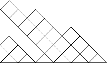
2.8. We will consider the lower region of $p$ not in the lower region of $p_{0}$ to be tiled with diamond tiles, and we will consider the lower region of $p$ intersecting the lower region of $p_{0}$ to be tiled with half-diamond tiles. For an example, see Figure 2.

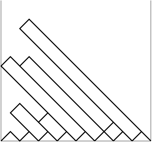
Proof: Given a sequence $\mathbf{r}=(r_{0},r_{1},\ldots,r_{n-1})$ of integers satisfying $0\leq r_{k}\leq 2k$ for $0\leq k\leq n-1$, we can form an overhang path in the following way. Start with the path $p_{0}$ described above. Then, for each $k$, add a rectangle $R_{k}$ to the $p_{0}$ with vertices $A_{k}=(2k,0),B_{k}=(2k+1,1),C_{k}=(2k-r_{k}+1,r_{k}+1)$ and $D_{k}=(2k-r_{k},r_{k})$ (this can be considered as a pile of $r_{k}$ diamonds piled up to the left of the step from $(2k,0)$ to $(2k+1,1)$ of $p_{0}$). The upper boundary of the union of these rectangles consists of steps of form (1) (corresponding to a line segment $D_{k}C_{k}$), form (2) (corresponding to part of a line segment $C_{k}B_{k}$ in the case where $r_{k}\geq r_{k+1}$ or $k=n$), or form (2’) (corresponding to part of a line segment $A_{k}D_{k}$ in the case where $r_{k}\leq r_{k-1}$). Hence this forms the lower region of an overhang path.

Conversely, given an overhang path, steps of form $(2)$ or $(2^{\prime})$ from $(a,b)$ do not change the sum $a+b$, while a step of form $(1)$ increases it by $2$. It follows that any overhang path must contain precisely $n$ steps of form $(1)$. By considering the diamond tiles down and to the right of these steps, we see that the path must be of the above form. It is clear that we now have a one-to-one correspondence between overhang paths and tuples of integers as above. The result follows. For an example, with $\mathbf{r}=(0,0,3,2,8,8,1,12)$, see Figure 3. $\Box$

2.9. For each $p\in\mathcal{G}_{n}$ there is a unique maximal path $t\leq p$ that only uses Dyck steps. We call this the root Dyck path (or just the root) of $p$. For example, in the introduction, the Dyck path example is the root of the overhang path example.

2.10. For $p\in\mathcal{G}_{n}$ and $q\in\mathcal{G}_{m}$ the side-by-side concatenation $p*q$ of $p$ and $q$ is a path in $\mathcal{G}_{n+m}$:

Note that not every path in $\mathcal{G}_{n+m}$ that passes through $(2n,0)$ arises in this way.

2.11. An element of $\mathcal{G}_{n}$ is said to be prime if it cannot be expressed non-trivially in the form $a*b$.

3.1. Given a finite set $S$, a pair partition of $S$ is a partition of $S$ into subsets of cardinality $2$. A Brauer diagram of degree $n$ is a picture of a pair partition of $2n$ distinct vertices arranged on the boundary of the lower half-plane. The two vertices in each part of the pair partition are joined by an arc in the lower half-plane. Two Brauer diagrams are identified if their underlying vertex pair partitions are the same. Let $J_{n}$ denote the set of all Brauer diagrams of degree $n$. See Figure 4 for an example. The additional arc and vertex labels are explained below.

3.2. We remark that Brauer diagrams are often defined using $2n$ vertices on the boundary of a disk or in a horizontal rectangle, with $n$ vertices along the top and $n$ vertices along the bottom, but we shall not consider such representations here.

3.3. By a partial Brauer diagram, we mean a Brauer diagram, but with the extra possibility that parts of cardinality $1$ are also allowed. We denote by $J_{n}^{l}$ the set of partial Brauer diagrams containing $n$ pairs and $l$ singletons (and thus a total of $2n+l$ vertices).

3.4. See Figure 12(a) for an example of a partial Brauer diagram which is not a Brauer diagram. We remark that a partial Brauer diagram can be completed on the left by adding another partial Brauer diagram to the left with the same number of singletons, and then pairing up the singletons in the first diagram with those in the second. Note that such a completion is in general not unique.

3.5. A TL diagram (or Temperley-Lieb diagram) is a Brauer diagram without crossings. We shall write $J_{n}^{TL}$ for the subset of $J_{n}$ consisting of TL diagrams.

3.6. Definition ((Right-)standard arc labelling).
Let $D$ be a partial Brauer diagram. We number the vertices of $D$ which are right-hand ends of arcs or singletons, in order from right to left. A vertex $k$ which is the right-hand end of an arc gets labelled $kR$, and we label the other end of the arc $kL$. Sometimes we will label the arc with endpoints $kL$ and $kR$ with the number $k$.

For an example, see Figure 4.

3.7. We define similarly a left-standard labelling, which again numbers from right to left, but according to the order of the left-hand endpoints of arcs (and singletons as before).

3.8. Later we will use the pair $(a(i),i)$ of left and right-standard labels for an arc in a fixed diagram $D$. That is, if $i$ is the right-standard label of an arc, then $a(i)$ will be the left-standard label of the same arc.

3.9. We will not need the, perhaps more natural, orderings from left to right. This handedness comes from the handedness of the overhang diagrams that we chose.

3.10. To each arc $i$ (in the right-standard labelling) of a diagram $D$ we may associate an arc (left) subdiagram $D^{i}$ of $D$. This is the collection of arcs whose right-hand vertex is strictly contained within arc $i$ (i.e. the interval from $iL$ to $iR$), together with their endpoints. We retain the initial (right-standard) labelling of the vertices inherited from $D$.

3.11. Example: Let $D$ be the diagram in Figure 4 above. The arc subdiagram $D^{1}$ is shown in Figure 5.

3.12. To any diagram $D$ in $J_{n}$ we may associate a diagram in $J_{n+1}$, denoted $[D]$, which is the diagram obtained from $D$ by adding a new vertex at each end of $D$, and an arc between them.

Similarly for $D\in J_{n}$ and $D^{\prime}\in J_{m}$ we will understand by $DD^{\prime}\in J_{n+m}$ the diagram obtained by simple side-by-side concatenation.

3.13. We shall call a diagram prime if it cannot be expressed non-trivially in the form $D=D_{1}D_{2}$. (This is a different definition of prime than has been used elsewhere, e.g. [L97, MS94]). Note that if a diagram $D$ is Temperley-Lieb and prime then it can be expressed in the form $D=[D^{\prime}]$.

4.1. There is a map from overhang paths to Brauer diagrams

defined by replacing each ‘blank’ tile with a patterned tile. Tiles in the root Dyck path of $p\in\mathcal{G}_{n}$ are replaced using the following rules:

or

Tiles in the lower region of $p$ but above the root of $p$ are replaced using the following rule:

A horizontal line above the overhang path is fixed (the “top” of the diagram). Strands are then connected together with vertical segments joining two ends, or joining an end with the top of the diagram. This can also be realised by continuing the tiling into the upper region of the path (up to the horizontal line), using half-tiles on the boundary, and using the following tiling rules for the new tiles:

For an example (with the tiles in the upper region omitted for clarity), see Figure 6.

4.2. We note that the patterned tiling of the lower part of $p$ in the above construction can be regarded as a pipe dream [FK96] (also known as an rc-graph [BB93]). In general it will be non-reduced, i.e. two arcs may cross twice in the resulting configuration (see the introduction for an example of this).

4.3. By the construction of $\Psi$, we have:

5.1. Note that the map $\Psi$ has image within the set of TL diagrams when restricted to the set of roots, given by ‘tiling’:

See e.g. [SW86].

5.2. The inverse of the restricted map is also well known. A convenient in-line representation of a TL diagram $D$ is to read from left to right and to replace each vertex that is the left hand end of an arc with an open bracket, ”(”, and to replace each vertex that is the right hand end of an arc with a close bracket, ”)”. It is clear that this gives rise to a well-nested sequence of brackets. Replacing each ”(” with a $1$ and each ”)” with a $2$ we obtain the in-line sequence for a Dyck path, call it $\Phi^{TL}(D)$.

5.3. By construction, we have the following:

Proof: This is implicit in [ABF84] (see [M91]), but we include a proof for the convenience of the reader. We show that for all TL-diagrams $D$, $\Psi(\Phi^{TL}(D))=D$. We do this by induction on $n$, with $n=0$ as base. Suppose that the result is true for smaller $n$. If $D$ is a TL diagram of degree $n$, suppose first that $D$ has an arc joining vertices $1$ and $2n$. Let $D^{\prime}$ be the TL-diagram obtained by removing this arc. By induction, $\Psi(\Phi^{TL}(D^{\prime}))=D^{\prime}$. It follows that $\Psi(\Phi^{TL}(D))=D$, since $\Phi^{TL}(D)$ is the same as the Dyck path $\Phi^{TL}(D^{\prime})$ except that an extra step $1$ at the start and an extra step $2$ at the end have been added.

If $D$ has no arc joining $1$ and $2n$ then it is of the form $D_{1}D_{2}$ where $D_{1}$ and $D_{2}$ are non-empty TL diagrams. By the inductive hypothesis, $\Phi^{TL}(\Psi(D_{i}))=D_{i}$ for $i=1,2$, and it follows that $\Phi^{TL}(\Psi(D))=D$. The result follows by induction.

It is well known that the cardinalities of $\mathcal{G}^{TL}_{n}$ and $J_{n}^{TL}$ are the same (given by the $n$th Catalan number), so the result follows. $\Box$

6.1. Our ultimate aim is to define a map

and show that it is inverse to $\Psi$. The difficulty is that the overhang path corresponding to a Brauer diagram may be hard to find. In the example given in the introduction, the realisation of the Brauer diagram obtained from the overhang path is not the simplest one: it contains more crossings than are necessary (one of the strings crosses one of the others twice: both crossings could be removed). Our approach will be to find first what will turn out to be the root of the desired overhang path and then add extra tiles to the corresponding Dyck path in order to give the required crossings.

Thus we will first of all define a map $\Pi:J_{n}\rightarrow J^{TL}_{n}$ associating a Temperley-Lieb diagram to each Brauer diagram. In the next section, we shall see that this gives us a useful labelling of each Brauer diagram. We will then study the properties of this labelling. This will give us control of the crossings and allow us to define $\Phi$. (The definition of $\Phi$ appears in Definition 9 and the main result is Theorem Theorem.)

6.2. The (right) chain $ch(D)$ of arcs of $D\in\mathcal{G}_{n}$ is the sequence $a_{1},a_{2},\ldots$ of arc labels of $D$ such that $a_{1}=1$ and $a_{i}$ (if it exists) is the arc label of the first right-hand end vertex to occur moving from right to left from the left-hand end vertex of the arc with label $a_{i-1}$.

6.3. Example: for the diagram in Figure 4, we have $ch(D)=(1,7)$ (in the right standard labelling); while $ch(D^{1})=(2,4)$ (borrowing the same labelling).

Note that the set of arcs in the chain $ch(D)$, together with the sets of arcs in the arc subdiagrams for the arcs in the chain (that are clearly disjoint sets), form the complete set of arcs of $D$.

6.4. Definition (Right chain tree of $D$).
Fix a diagram $D$. Firstly, for each arc $i$ of $D$ define a planar rooted tree with root $i$ and other vertices the chain arcs of $D^{i}$ arranged in right chain order, right to left, at tree distance 1 from the root. For example, for the arc $1$ in Figure 4, we obtain:

Note that the second row contains the right chain arcs of $D^{1}$ given above. Define a planar rooted tree $\tau_{R}(D)$ with vertices the arcs of $D$ together with a root vertex $\emptyset$. The tree is obtained by concatenating the planar rooted trees for the right chain arcs of $D$ in the obvious way, setting $D^{\emptyset}=D$ to include the root. We call this tree the right chain tree of $D$. We have thus defined a map $\tau_{R}$ from $J_{n}$ to planar rooted trees.

6.5. Example: The right-chain tree for our example $D$ above is shown in Figure 7.

6.6. Let $\gamma$ denote the usual geometric dual map from planar rooted trees to TL diagrams. Thus, for a planar tree $T$, each arc of the TL diagram $\gamma(T)$ passes through a unique edge of $T$. The dual TL diagram for the above example is shown in Figure 8.

Combining, we have a map

6.7. Note that the right standard labelling of the arcs of $D$ coincides with the labelling of the vertices of $\tau_{R}(D)$ in order of first meeting, moving counterclockwise around the tree from the root. An example of this can be seen in Figure 8, where the arc ends are given their right standard labels.

Note also that applying the map $\Phi^{TL}$ to $\Pi(D)$ gives a Dyck path. So we can also associate a Dyck path to each Brauer diagram. For our example the Dyck path is shown in Figure 9.

6.8. Note that the left-standard labelling of arcs in a TL diagram induces a labelling for steps of form (1) in the associated Dyck path, whereby each such step is given the label of the arc passing through it. See Figure 10 for an example.

7.1. In this section we will show how the right-standard labellings of the arcs of $D$ and $\Pi(D)$ can be used to obtain a new labelling (which we call secondary labelling) of the arcs of $D$, by transferring the left-standard labelling of $\Pi(D)$ to $D$. We shall see later how the ordering on the arcs determined by this secondary labelling can be used to uncross the arcs of $D$ to get $\Pi(D)$; this is a key notion in the construction of the map $\Phi$.

7.2. Fix a Brauer diagram $D$. Each arc of the TL diagram $\Pi(D)$ has a pair $(a(i),i)$ of left and right-standard labels. Thus for each right-standard label $i$ there is a corresponding left-standard label $a(i)$.

For example, in the TL diagram in Fig 11(b), we have $a(3)=1$.

7.3. Definition (Secondary arc label).
For each arc $i$ in $D$ there is an arc in $\Pi(D)$ with the same right-standard label. We call this association between arcs of $D$ and arcs of $\Pi(D)$ the ‘right-correspondence’. We now associate a new ‘secondary’ label to each arc in $D$ — the left-standard label for the right-corresponding arc in $\Pi(D)$.

7.4. For example, the secondary-labelling for the diagram $D$ in Figure 4 is shown in Figure 11(a). The labels at the top of the diagram are the right-standard labels, and each arc has been given its left-standard label. We remark that if $D\in J_{n}^{TL}$ then $\Pi(D)=D$, so its secondary and left-standard labels coincide.

7.5. Definition (Right-agreement).
Let us say that two diagrams right-agree up to a given vertex $x$ if there is a partial Brauer diagram on that vertex and the vertices to the right of it which can be completed on the left to either of the two diagrams. If, in addition, the two diagrams do not right-agree up to the vertex immediately to the left of $x$, we shall say that they maximally right-agree up to $x$.

7.6. See Figure 12 for an example. Diagrams (b) and (c) right-agree up to the fifth vertex from the right since the partial Brauer diagram (a) can be completed to either of them. It is clear that in fact the two diagrams maximally right-agree up to this vertex. Note also that $\Pi(D)$ and $D$ in Figure 11 maximally right-agree up to the third vertex from the right (labelled $3R$ in both diagrams).

7.7. Lemma. Suppose that $D$ and $\Pi(D)$ right-agree up to a given vertex $x$. Suppose that there is an arc of $D$ in the agreeing part. Then the right-corresponding arc in $\Pi(D)$ is also in the agreeing part (indeed, this is the same pair of vertices in the pair partition). These arcs have the same secondary label. Furthermore, the set of these agreeing labels (if any) is of the form $\{1,2,\ldots,r\}$ for some $r$.

Proof: Let $E$ be the partial Brauer diagram which can be completed to either $D$ or $\Pi(D)$ (on the vertex $x$ and all vertices to its right). It follows from the definitions that the right-standard labels on the vertices and the left-standard labels on the arcs of $E$ are the same in either completion.

Thus, on completion, an arc in $E$ gives rise to a right-corresponding pair of arcs in $D$ and $\Pi(D)$. By the definition of the secondary labels, the arc in $D$ will have secondary label equal to the left-standard label of the (right-corresponding) arc in $\Pi(D)$.

The consecutive property follows immediately from the definition of left-standard labels. $\Box$

7.8. Lemma. Let $D\in J_{n}$, and suppose that the left hand end of the arc with right-standard labels $aL$ and $aR$ is to the right of the right-hand end of the arc with right-standard labels $bL$ and $bR$. Let $i$ be the secondary label of the former arc and $j$ the secondary label of the latter arc. Then in $\tau_{R}(D)$, $i$ and $j$ are not descendants of each other.

Proof: By the definition of $\tau_{R}(D)$, the descendants of $j$ arise from (some of) the arcs whose right hand end lies between the ends of $i$, and cannot include $j$ by assumption. Similarly $i$ cannot be a descendant of $j$. $\Box$

8.1. In this section we study the relationship between $D$ and $\Pi(D)$; we shall use these results to define $\Phi$ in the next section.

8.2. Lemma. Let $D\in J_{n}$, and suppose that $D$ and $\Pi(D)$ maximally right-agree up to vertex $x$. Then the vertex $y$ immediately to the left of $x$ is the left hand end of an arc in both $D$ and $\Pi(D)$.

Proof: Case (I): If $y$ were the right-hand end of an arc in both $D$ and $\Pi(D)$ then $D$ and $\Pi(D)$ would right-agree up to vertex $y$, a contradiction to the assumption. We complete the proof by ruling out the two remaining undesirable configurations, i.e. the configurations in which $y$ is a left-hand end of an arc only in $D$ or only in $\Pi(D)$.

Case (II): Suppose that $y$ is the left-hand end of an arc in $D$ but the right-hand end of an arc in $\Pi(D)$. Let $aL$ and $aR$ be the right-standard labels of the arc in $D$ incident with $y$ in $D$ and let $bL$ and $bR$ be the right-standard labels of the arc incident with $y$ in $\Pi(D)$. Note that $aR$ must be $x$ or to its right in $D$, so the vertex with right-standard label $aR$ in $\Pi(D)$ must also be $x$ or to the right of $x$, since $D$ and $\Pi(D)$ right-agree up to vertex $x$, using Lemma 7. For the same reason, the vertex with right-standard label $aL$ in $\Pi(D)$ must be to the left of $x$, since this is so in $D$. Since vertex $y$ is labelled $bR$ and the arcs in $\Pi(D)$ do not cross, the vertex with right-standard label $aL$ in $\Pi(D)$ must be to the left of $bL$.

The vertex with right-standard label $bR$ in $D$ must be to the left of $x$, since this is so in $\Pi(D)$ (again using Lemma 7), so, since $y$ is right-standard labelled $aL$ in $D$, the vertex with right-standard label $bR$ in $D$ must be to the left of the vertex with right-standard label $bL$ in $D$. Let $i$ (respectively, $j$) be the secondary label of the arc with end-points $aL$ and $aR$ (respectively, $bR$ and $bL$) in $D$. By Lemma 7, $i$ and $j$ are not descendants of each other in $\tau_{R}(D)$. But this contradicts the fact that the right-corresponding arcs (also labelled $i$ and $j$) in $\Pi(D)$ are nested. See Figure 13. The dashed vertical line is drawn between vertices $x$ and $y$ (so the right-agreeing part of $D$ and $\Pi(D)$ is to the right of this line).

Case (III): Suppose that $y$ is the right-hand end of an arc in $D$ but the left-hand end of an arc in $\Pi(D)$. Let $aL$ and $aR$ be the right-standard labels of the arc in $D$ incident with $y$ in $\Pi(D)$ and let $bL$ and $bR$ be the right-standard labels of the arc incident with $y$ in $D$. Note that $aR$ must be $x$ or to its right in $\Pi(D)$, so the vertex with right-standard label $aR$ in $\Pi(D)$ must also be $x$ or to the right of $x$, since $D$ and $\Pi(D)$ right-agree up to vertex $x$, using Lemma 7.

Since the vertex with right-standard label $bR$ in $D$ is to the left of $x$, its right-correspondent in $\Pi(D)$ must also be to the left of $x$ (using Lemma 7) and thus the whole of the arc with right-standard labels $bL$ and $bR$ must be to the left of the vertex with right-standard label $aL$ in $\Pi(D)$. Let $i$ (respectively, $j$) be the secondary label of the arc with end-points $aL$ and $aR$ (respectively, $bR$ and $bL$) in $D$. These are the left-standard labels of the right-corresponding arcs in $\Pi(D)$, and by the above neither is a descendant of the other in $\tau_{R}(D)$ by the definition of $\Pi(D)$.

We claim that, using the definition of $\tau_{R}(D)$, $j$ is a descendant of $i$ in $\tau_{R}(D)$: a contradiction. Since $\Pi(D)$ and $D$ right-agree up to vertex $x$, the diagram for $D$ can be drawn with no crossings to the right of a vertical line $V$ drawn between vertices $x$ and $y$.

Let $a_{1}R,a_{2}R,\ldots,a_{k}R$ be the right-hand end-points of the arcs of $D$ with right-hand end-point at $x$ or to its right and left-hand end-point to the left of $x$, with $a_{1}<a_{2}<\cdots<a_{k}$. Note that the left-hand end-point of each of these arcs is to the left of the vertex with right-standard label $bR$ in $D$. It follows that arc $j$ is in the subdiagram $D^{a_{1}}$.

It follows similarly that arc $j$ is in the subdiagram $D^{a_{2}}$, and by continuing to argue in this way we eventually obtain that arc $j$ is in the subdiagram $D^{i}$ and thus is a descendant of $i$ as required. See Figure 14.

We have thus ruled out all other possible configurations and can conclude that the lemma holds. $\Box$

8.3. Lemma. Let $D\in J_{n}$, and suppose that $D$ and $\Pi(D)$ maximally right-agree up to a vertex $x$. Let $y$ be the vertex immediately to the left of $x$ and let $z$ be the vertex immediately to the left of $y$. Then $z$ is the left hand end-point of an arc in $\Pi(D)$.

Proof: For a contradiction, we suppose that the vertex $z$ in $\Pi(D)$ is the right-hand end of an arc. Let its right-standard label be $cR$. The vertex which is right-standard labelled $cR$ in $D$ must occur to the left of vertex $x$ in $D$, as it does in $\Pi(D)$. Let $dL$ be the right-standard label of the vertex $y$ in $D$ (note that by Lemma 8 this vertex must be the left-hand end-point of an arc in $D$).

We see that:

(*) The vertex with right-standard label $cR$ in $D$ occurs to the left of the vertex with right-standard label $dL$.

The right-hand end of the arc incident with $dL$ must be either $x$ or to the right of $x$ in $D$. This vertex is labelled $dR$. Then the vertex with right-standard label $dL$ must be to the left of $x$ in $\Pi(D)$ and the vertex with right-standard label $dR$ must be $x$ or to the right of $x$ in $\Pi(D)$ (as both of these hold for the right-corresponding vertices in $D$).

Since $\Pi(D)$ has no crossings of arcs, the vertex with right-standard label $dR$ in $\Pi(D)$ must be to the right of the vertex right-standard labelled $bR$ in $\Pi(D)$ and the vertex with right-standard label $dL$ in $\Pi(D)$ must be to the left of the vertex with right-standard label $cL$ in $\Pi(D)$. Thus

(**) In $\Pi(D)$, the arc with end-points $dL$ and $dR$ contains the arc with end-points $cL$ and $cR$.

Let $i$ (respectively, $j$) be the secondary label of the arc with end-points $bL$ and $bR$ (respectively, $cL$ and $bR$) in $D$. Let $k$ be the secondary label of the arc with end-points $dL$ and $dR$ in $D$; this coincides with the left-standard label of the arc in $\Pi(D)$ with these end-points, by the definition of secondary label. Then by (**) above and the definition of $\Pi(D)$, $j$ is a descendant of $k$ in $\tau_{R}(D)$. But by (*) and Lemma 7, $j$ is not a descendant of $k$ in $\tau_{R}(D)$, a contradiction.

It follows that vertex $z$ must be the left hand end-point of an arc in $\Pi(D)$ as required. $\Box$

9.1. In this section we will define the map $\Phi:J_{n}\rightarrow\mathcal{G}_{n}$ and show that it is an inverse to the tiling map $\Psi$, thus proving our main result, that there is a bijection between overhang paths and Brauer diagrams. We first need a key lemma:

9.2. Lemma. Let $D\in J_{n}$, and suppose that $D$ and $\Pi(D)$ maximally right-agree up to vertex $x$. Let $r$ be as in Lemma 7. Then:
(a) The right hand ends of the arcs in $D$ and $\Pi(D)$ with secondary label $r+1$ lie in the right-agreeing right-hand-end of the two diagrams. (b) The left-hand end of the arc with secondary label $r+1$ in $D$ is further from the right-hand end of $D$ than the left-hand end of the arc with the same left-standard (i.e. secondary) label in $\Pi(D)$.

Proof: The arc whose left-hand end-point is immediately to the left of vertex $x$ in $\Pi(D)$ (see Lemma 8) has left-standard (i.e. secondary) label $r+1$ by definition of left-standard labelling. Therefore its right-hand end-point is in the right-agreeing part of $D$ and $\Pi(D)$. The arc in $\Pi(D)$ with secondary label $r+1$ is the right-corresponding arc in $D$. Since $D$ and $\Pi(D)$ right-agree up to $x$, its right-hand end must also lie in the right-agreeing part, and (a) is shown. Since $D$ and $\Pi(D)$ maximally agree up to vertex $x$, the left-hand end of the arc with secondary label $r+1$ in $D$ cannot be the vertex immediately to the left of vertex $x$, but it cannot be in the right-agreeing part of $D$ and $\Pi(D)$ since the left-hand end of the right-corresponding arc in $\Pi(D)$ does not lie in this right-agreeing part. The result follows. $\Box$

9.3. Let $X_{D}$ denote the number of steps to the right that the left hand end of arc with secondary label $r+1$ in $D$ in Lemma 9 above would have to be moved in order to right-agree with that arc in $\Pi(D)$. Define $\delta D$ to be the diagram resulting from moving the left-hand end of the arc with secondary label $r+1$ in this way.

9.4. For example, if $D$ is the diagram in Figure 11(a), then $r=0$ and $D$ and $\Pi(D)$ maximally right agree up to the third vertex from the right. Since moving the left hand end point of the arc with secondary label $1$ in $D$ five steps to the right would make it right agree with the arc with the same label in $\Pi(D)$, we have $X_{D}=5$.

9.5. This means that $\delta D$ and $\Pi(D)$ exhibit greater right-agreement, that is, right-agreement up to a vertex to the left of the right-agreeing part of $D$ and $\Pi(D)$. (Note that in the example, $\delta D$ and $\Pi(D)$ maximally right-agree on the nine rightmost vertices). We define $D(r)=D$ and $X_{r}=X_{D}$. Next we define $D(r^{\prime})=\delta D$ and $X_{r^{\prime}}=X_{\delta_{D}}$ (where $r^{\prime}$ is as in Lemma 7 for $\delta D$), and so on, iterating the procedure. We thus obtain a sequence

For any $j$ not appearing in this sequence (i.e. no adjustment is required to bring the arcs with secondary label $j+1$ into right-agreement), we define $D(j)$ to be $D(s)$, where $s$ is minimal with the property that the arcs with secondary label $j+1$ agree in $D(s)$ and $\Pi(D)$. In such cases, we set $X_{j}=0$.

9.6. Each single step counted by $X_{D}=X_{r}$ can be implemented on $D$ by an adjacent pair permutation of vertices. Thus by extending the diagram above to include a single crossing $\sigma_{j(r)}$ (say) in the appropriate position, for each such step, we can build up the transformation $D\rightarrow\delta D$. We repeat this procedure for each transformation in the above sequence.

In our example, the extension for the first transformation is shown in Figure 15.

9.7. Of course $\sigma_{j(i)}^{2}=1$, so applying the collection of these changes in reverse order to $\Pi(D)$ brings us to $D$.

9.8. Definition (The inverse map, $\Phi$).
Given a Brauer diagram, $D$, let $\Phi(D)$ be the diagram obtained by starting from the Dyck path $\Phi^{TL}(\Pi(D))$ for $\Pi(D)$ and, for each $i$, appending to the step in the Dyck path of form $(1)$ with label $i$ a left-overhanging stack of tiles of length $X_{D(i)}$. We remark that it follows from Lemma 8 that $\Phi(D)$ is an overhang path.

9.9. It follows from the above that applying $\Psi$ to $\Phi(D)$ we obtain the original diagram $D$. (An example follows shortly).

9.10. It is well known (see also Section 11) that the cardinality of $J_{n}$ is equal to $(2n-1)!!$ so it follows from Lemma Lemma that $|J_{n}|=|\mathcal{G}_{n}|$. We have therefore shown that:

10.1. We now give an example demonstrating the main theorem.

10.2. Let $D$ be the Brauer diagram in Figure 11(a). We have seen already that $\Pi(D)$ is the TL diagram in Figure 11(b), and that $D$ and $\Pi(D)$ maximally right agree up to the third vertex from the right, including $r=0$ arcs in their entirety. Thus we write $D(0)=D$. We have seen that $X_{D}=X_{0}=5$, so we first move the arc secondary labelled $1$ five steps to the right to obtain diagram $\delta D$; see Figure 16.

10.3. We observe that $\delta D$ and $\Pi(D)$ maximally agree up to the ninth vertex from the right, including the arcs secondary-labelled $1$. In fact the arcs secondary-labelled $2$ and $3$ also right-agree, so $r^{\prime}=3$ and we write $\delta D=D(3)$ (thus $D(1)=D(2)=\delta D$). By moving the arc secondary-labelled $r^{\prime}+1=4$ three steps to the right we can make it right-agree with the arc with the same secondary label in $\Pi(D)$, giving the diagram $\delta D(3)$ shown in Figure 17. Thus $X_{3}=3$.

10.4. We see that the arcs secondary-labelled $1,2,3,4$ lie in the right-agreeing parts of $\delta D(3)$ and $\Pi(D)$, so $\delta D(3)=D(4)$. We compute that $X_{4}=5$ and diagram $\delta D(4)$ is shown in Figure 18.

10.5. Next, the arcs secondary-labelled up to $6$ lie in the right-agreeing parts of $\delta D(4)$ and $\Pi(D)$, so $\delta D(4)=D(6)$. We compute that $X_{6}=1$ and $\delta D(6)=\Pi(D)$.

10.6. Using this data to construct $\Phi D$ we obtain the overhang path in Figure 19. Note that the tiling of this path does indeed return $D$.

11.1. In this section we give a simple bijection between overhang paths and Brauer diagrams, also given by tiling. We note, however, that it does not have the property that it restricts to the tiling bijection for the Temperley-Lieb case, described in Section 5.

Let $n\in\mathbb{N}$. Recall that $J_{n-1}^{1}$ denotes the set of partial Brauer diagrams with $n-1$ pairs and one singleton. There is a bijection

given by deleting the rightmost vertex of a Brauer diagram. The inverse adds a single vertex at the right hand end and joins it with the singleton. There is a map from $J_{n-1}^{1}$ to $J_{n-1}$ obtained by deleting the singleton. There are $2n-1$ possibilities for the singleton, giving a bijection:

where $\underline{k}$ denotes the set $\{1,2,\ldots,k\}$ for any $k$. Thus $d_{2n}:=s_{-}\circ s_{2n}$ is a bijection from $J_{n}$ to $J_{n-1}\times\underline{2n-1}$. It follows that

and thus that $|J_{n}|=(2n-1)!!$. It follows from the above that

where

is a bijection.

11.2. In this section only, we shall regard a Dyck path as a walk on $\mathbb{Z}\times\mathbb{Z}$ from $(0,0)$ using steps from $\{(1,0),(0,1)\}$, such that the walk never drops below the line parallel to the vector $(1,1)$ (equivalently, if the height of a point $(x,y)$ is defined to be $y-x$, negative heights are not allowed). It is clear that such a path can be transformed into a Dyck path as defined in Section 2 by rotating it through $45$ degrees clockwise about the origin and stretching it by a factor of $\sqrt{2}$. We consider such paths whose end-point is $(n,n)$.

11.3. Similarly, in this section only, we shall regard an overhang path as a generalisation of such a walk in which steps of the form $(-1,0)$ are also allowed, but the walk also never drops below (i.e. to the left of) the line defined by the $(-1,1)$ vector (and the path may not visit the same vertex twice). Such a path is characterised by the sequence of $x$-coordinates of its $(0,1)$-steps. The first entry in this sequence is necessarily $0$, the second lies in $\{-1,0,1\}$, the third lies in $\{-2,-1,0,1,2\}$, and so on. (In the Dyck path case the negative positions do not occur.) Let $O_{n}$ denote the set of such paths ending at $(n,n)$.

11.4. It is clear that there is a bijection from $A_{n}$ to $O_{n}$ taking an element $(x_{1},x_{2},\ldots,x_{n})$ of $A_{n}$ to the overhang path with sequence of $x$-coordinates of its $(0,1)$-steps given by $x_{i}-i$, $i=1,2,\ldots,n$.

11.5. We have thus constructed a bijection

One way to construct the inverse of the above bijection is to start with an element of $O_{n}$ and to regard this as a partial tiling of the plane with $1\times 1$ tiles. That is, one fills the interval between a given overhang path and the lowest path with tiles. One also tiles the interval between the $(1,1)$ line and the lowest path with half-tiles in the obvious way. One then decorates all the square tiles with crossed lines from edge to opposite edge; and the triangular tiles each with a single line from short edge to short edge. This decoration gives the corresponding element of $J_{n}$.

12.1. In this section we explain how Dyck paths and related walks arise in the representation theory of the Hecke algebra, via representations arising from outer product representations of the symmetric group.

12.2. Fix $q\in\mathbb{C}$ and $n\in\mathbb{N}$. Let $H_{n}=H_{n}(q)$ denote the usual Hecke algebra of degree $n$ over $\mathbb{C}$ (we work over $\mathbb{C}$ for simplicity). Thus $H_{n}$ is the $\mathbb{C}$-algebra with generators $g_{1},g_{2},\ldots g_{n-1}$ subject to relations $g_{i}g_{j}=g_{j}g_{i}$ if $|i-j|>1$, $g_{i}g_{j}g_{i}=g_{j}g_{i}g_{j}$ if $|i-j|=1$, and $(g_{i}+q^{2})(g_{i}-1)=0$.

12.3. Definition. For $d\in\mathbb{N}$, we denote by $\Gamma^{d}_{n}$ the set of all $d$-tuples $\lambda=(\lambda^{1},\lambda^{2},...,\lambda^{d})$ of Young diagrams, with $|\lambda|=\sum_{i=1}^{d}|\lambda^{i}|=n$.

Fix $\lambda\in\Gamma^{d}_{n}$. Then a tableau of shape $\lambda$ is any arrangement of the ‘symbols’ $1,2,..,n$ in the $n$ boxes of $\lambda$. Such a tableau is said to be standard if each component tableau is standard. We denote the set of all standard tableaux of shape $\lambda$ by $T^{\lambda}$.

12.4. We number the rows of $\lambda$ by placing the whole of the component diagram $\lambda^{i+1}$ under $\lambda^{i}$ for all $i$, and numbering the rows from top to bottom. We then define a total order $<$ on standard tableaux of shape $\lambda$ by setting $T<U$ if the highest number which appears in different rows of $T$ and $U$ is in an earlier row in $U$.

12.5. Let $T$ be a tableau. For $i\in\{1,2,\ldots,n-1\}$, let $\sigma_{i}=(i\ i+1)\in\Sigma_{n}$, the symmetric group of degree $n$. We define $\sigma_{i}(T)$ to be the tableau obtained by interchanging $i$ and $i+1$. In this way we get an action of $\Sigma_{n}$ on the set of all tableaux of shape $\lambda$, but we note that this action does not necessarily take a standard tableau to a standard tableau.

12.6. Let $x=(x_{1},x_{2},\ldots,x_{d})\in\mathbb{R}^{d}$. For $i,j\in\{1,2,\ldots,n-1\}$ and $T\in\Gamma^{d}_{n}$ let $h^{x}_{ij}=h^{x}_{ij}(T)$ denote the generalised hook length between the symbols $i$ and $j$ in $T$. Thus $h^{x}_{ij}$ is given by:

where $h^{0}_{ij}$ is the usual hook length obtained by superimposing the component tableaux of $T$ containing $i$ and $j$, and $\#i$ is the number of the component containing $i$ in $T$. See [MWL00] (note that there is a typographical error in this paper at the relevant point) and also [M91, p.244]. Geometrically, one may think of putting all the individual Young diagrams $\lambda^{i}$ in the same plane, each with its top left box in position $(0,x_{i})$.

For an integer $m$, we will write, as usual,

12.7. Proposition [MWL00]. Let $\lambda\in\Gamma^{d}_{n}$ and assume that $[h_{i,i+1}^{x}(T)]\not=0$ for all $i\in\{1,2,\ldots,n-1\}$ and all $T\in T^{\lambda}$. Then the set $T^{\lambda}$ is a basis for a left $H_{n}$–module $R^{\lambda}$. For $i\in\{1,2,\ldots,n-1\}$ and $T\in T^{\lambda}$, the action is as follows:
(a) If $i,i+1$ lie in the same row of $T$ then $g_{i}T=T$.
(b) If $i,i+1$ lie in the same column of $T$ then $g_{i}T=-q^{2}T$.
(c) If neither (a) nor (b) hold, then $\sigma_{i}(T)$ is also standard. Let $h=h_{i,i+1}^{x}$. Then the action is given by

provided $T<\sigma_{i}(T)$.

(Young’s orthogonal form (see e.g. [Bo70, IV.6]) involves an action via symmetric matrices related to those above via conjugation).

12.8. We now restrict attention to the situation in which $\lambda$ has exactly two components, each consisting of exactly one row. We can represent $T\in T^{\lambda}$ by an $n$-tuple $(a_{1},a_{2},\ldots,a_{n})$ with entries in $\{1,2\}$, defined by the condition that $i\in\lambda^{a_{i}}$ for all $i\in\{1,2,\ldots,n\}$. Such a tuple can be regarded as a walk of length $n$ in $\mathbb{Z}^{2}$ starting at the origin. The $i$th step of the walk consists of adding the vector $(1,1)$ if $a_{i}=1$ or adding the vector $(1,-1)$ if $a_{i}=2$.

References

- [ABF84] G. E. Andrews, R. J. Baxter and P. J. Forrester, Eight-vertex SOS model and generalized Rogers-Ramanujan-type identities. J. Statist. Phys. 35 (1984), no. 3–4, 193–266.
- [BF01] T. H. Baker and P. J. Forrester, Random walks and random fixed-point free involutions. J. Phys. A: Math. Gen. 34 (2001), L381–L390.
- [BB93] N. Bergeron and S. Billey, RC-graphs and Schubert polynomials. Experimental Mathematics 2, No. 4 (1993), 257–269.
- [Bo70] H. Boerner, Representations of groups. With special consideration for the needs of modern physics. Translated from the German by P. G. Murphy in cooperation with J. Mayer-Kalkschmidt and P. Carr. 2nd. English ed., North-Holland Publishing Co., Amsterdam-London; American Elsevier Publishing Co., Inc., New York, 1970.
- [Br37] R. Brauer, On algebras which are connected with the semisimple continuous groups. Ann. of Math. (2) 38 (1937), no. 4, 857–872.
- [CDDSY07] W. Y. C. Chen, E. Y. P. Deng, R. R. X. Du, R. P. Stanley and C. H. Yan, Crossings and nestings of matchings and partitions. Trans. Amer. Math. Soc. 359 (2007), no. 4, 1555–1575.
- [CDM09] A. Cox, M. De Visscher, P. Martin, A geometric characterisation of the blocks of the Brauer algebra. J. Lond. Math. Soc. (2) 80 (2009), no. 2, 471–494.
- [CDM10] A. Cox, M. De Visscher and P. P. Martin, Alcove geometry and a translation principle for the Brauer algebra, Journal of Pure and Applied Algebra, doi:10.1016/j.jpaa.2010.04.023, 2010.
- [CDM] A. Cox, M. De Visscher and P. P. Martin, private communication, 2010.
- [DM93] M. R. T. Dale and J. W. Moon, The permuted analogues of three Catalan sets. J. Statist. Plann. Inference 34 (1993), no. 1, 75–87.
- [FK96] S. Fomin and A. N. Kirillov, The Yang-Baxter equation, symmetric functions, and Schubert polynomials. Discrete Math. 153 (1996), 123–143.
- [HL04] T. Halverson and T. Lewandowski, RSK insertion for set partitions and diagram algebras. Electron. J. Combin. 11 (2004/06), no. 2, Research Paper 24, 24 pp.
- [L97] W. B. R. Lickorish, An introduction to knot theory. Graduate Texts in Mathematics, 175. Springer-Verlag, New York, 1997.
- [MM] R. J. Marsh and P. Martin, Pascal arrays: counting Catalan sets. Preprint arXiv:math/0612572v1 [math.CO], 2006.
- [M91] P. Martin, Potts models and related problems in statistical mechanics. World Scientific, Series on Advances in Statistical Mechanics, Volume 5, 1991.
- [M09] P. P. Martin, The decomposition matrices of the Brauer algebra over the complex field. Preprint arXiv:0908.1500v1 [math.RT], 2009.
- [MR98] P. P. Martin and G. Rollet, The Potts model representation and a Robinson-Schensted correspondence for the partition algebra. Compositio Math. 112 (1998), no. 2, 237–254.
- [MWL00] P. Martin, D. Woodcock and D. Levy, A diagrammatic approach to Hecke algebras of the reflection equation. J. Phys. A 33 (2000), no. 6, 1265–1296.
- [MS94] P. Martin and H. Saleur, On algebraic diagonalization of the chain. Perspectives on solvable models. Internat. J. Modern Phys. B 8 (1994), no. 25-26, 3637–3644.
- [R] M. Rubey, Nestings of Matchings and Permutations and North Steps in PDSAWs. Preprint arXiv:0712.2804v4 [math.CO].
- [Sl09] N. J. A. Sloane, (2009), The On-Line Encyclopedia of Integer Sequences. www.research.att.com/ njas/sequences/.
- [SW86] D. Stanton and D. White, Constructive combinatorics. Undergraduate Texts in Mathematics. Springer-Verlag, New York, 1986.
- [Su86] S. Sundaram, On the combinatorics of representations of . Ph.D. Thesis, M.I.T., 1986.
- [Su90] S. Sundaram, The Cauchy identity for . J. Combin. Theory Ser. A 53 (1990), 209–238.
- [TL71] H. N. V. Temperley and E. H. Lieb, Relations between the “percolation” and “colouring” problem and other graph-theoretical problems associated with regular planar lattices: some exact results for the “percolation” problem. Proc. Roy. Soc. London Ser. A 322 (1971), no. 1549, 251–280.
- [T01] I. Terada, Brauer diagrams, updown tableaux and nilpotent matrices. J. Alg. Comb. 14 (2001), 229–267.