3-Form Flux Compactification of Salam-Sezgin Supergravity
The compactification of 6 dimensional Salam-Sezgin model in the presence of 3-form flux is investigated. We find a torus topology for this compactification with two cusps which are the places of branes, while at the limit of large size of the compact direction we also obtain sphere topology. This resembles the Randall-Sundrum I,II model. The branes at one of the cusps can be chosen to be 3- and 4-branes which fill our 4-dimensional space together with the fact that at this position restores the Lorentz symmetry. This compactification also provides an example for the so-called ‘time warp’ solution, [0812.5107 [hep-th]]. According to a no-go theorem in , the time warp compactification violates the null energy condition. While the theorem is quiet for , our model gives a time warp compactification which satisfies the null energy condition. We also derive the four dimensional effective Planck mass which is not obvious due to the time warp nature of the solution.
| IPM/P-2009/021 |
1 Introduction
In more than a decade, since the celebrated work of Randall-Sundrum [1, 2], the warp compactification, has been considered as a new approach to explain the hierarchy problem in 4-dimensional space-time as a low energy limit of higher dimensional theories. This approach brought new phenomenological results with more hopes to find evidences for higher dimensional theories in a foreseeable future.
Long before the warp compactification idea, the six dimensional gauged supergravity was studied by Salam-Sezgin in [3, 4, 5, 6], as a simple model to obtain the supersymmetric vacua by compactification to 4 dimensions. It has also interesting applications in cosmological model building [7, 8, 9, 10]. On the other hand, in another development [11], it has been shown that this model can be derived from the string theory which strengthens its importance as a descendent of a fundamental theory. In a modern view, the Salam-Sezgin supergravity is rich enough, while simple, to provide the warp compactification including fluxes [12, 13, 14, 15, 16, 17, 18]. In [17], it was found that four dimensional Minkowski space solution is not only possible, but inevitable if one requires maximal symmetry in four dimensions and compactness of internal space. Based on these features, it is worth to work out its various warp compactifications.
The bosonic part of the model contains the metric, dilaton, a 2-form and a 3-form as field strengths. In [12, 13, 14, 15, 16, 17, 18, 19] a static warped solution has been found for and . A dynamical model was proposed in [20]. For some recent developments see [21, 22, 23]
In all of the case, so far has been set to zero. Beside technical reasons which make equations hard to solve when is included, it is obvious that the presence of a 3-form in a 6-dimensional space can not support a symmetric 4-dimensional compactification. Nonetheless, we will see soon that the situation is not a disaster and one may find an appropriate interpretation.
In this paper, we have considered a 4-dimensional compactification with field which is extended along the 2-dimensional internal space and the time direction. This kind of discrimination between time and other non-compact spatial directions, may suggest its application to cosmological models, however, here we restrict ourselves to a static model and postpone the study of dynamical solutions to future. Should we need a warp compactification, field configuration suggests the warp factors in time and spatial directions should be different. This is what has been called ‘time warp’ recently in [24]. The ratio of time and spatial warp factor is the light speed which depends on the internal coordinate by construction. There is a no-go argument in [24] according to which the internal space in time warped solutions can not be compact, unless the null energy condition is violated. Meanwhile the validity of this no-go theorem in is under query, and indeed our model provides a counterexample in which the null energy condition can be satisfied even for the compact case.
We show that it is needed to solve equations in different patches and join them by Israel junction conditions [25]. These conditions could be satisfied only when one introduces the branes at joining positions [26]. In this way we find out branes sitting at the middle and two ends of the compact space. More explicitly, we consider a compact internal space with axial symmetry which satisfies equations of motion in the interval for the radial coordinate, , and then extended to interval with and identified. Thus we have a torus topology, with two cusps at 0 and which are the positions of branes. We consider minimal number of branes and show that it is possible to introduce 3- and 4-branes filling our 4-dimensional space where the 4-brane wrapped and 3-branes are smeared over the internal circle [27]. On the other side at , in addition to 3- and 4-branes, we need 0-branes to satisfy the junction conditions with time-space asymmetry. These 0-branes smeared over the world volume of the 4-brane. This configuration makes it possible to have a 4-dimensional symmetric space at . To ensure about this symmetry we need to consider the behavior of field at . Indeed is discontinuous at this position, since branes act as a surface of polarized charges for the electrical field, so the field changes the sign while crossing the brane. The mean value of would be zero at which together with the branes configuration restore the 4-dimensional lorentz symmetry at .
At the first look, it may seem impossible to introduce an effective covariant 4-dimensional gravity, however, a fine tuning of the parameters make it possible to obtain the effective Planck mass and 4-dimensional symmetry in the linear approximation.
We organize the paper as follows. In the next section, equations of motion including the metric, dilaton and field are solved. In section 3, we introduce the junction conditions and branes. These conditions also fix some of the integration constants and we discuss the domain of independent parameters. The section 4 is devoted to discuss the large limit where depending on the parameters, the internal azimuthal radius may diverge or shrink at large to give new topologies. In section 5, we show the validity of the null energy condition. In section 6, the effective four dimensional gravity is considered and the effective Planck mass is derived. We conclude in section 7.
2 Equations of motion and -flux solution
Let us start with the bosonic part of generalized Salam-Sezgin model with the following Lagrangian[3, 4, 5, 6]:
| (2.1) |
where capital latin indices are six dimensional indices, is the dilaton, and are 2 and 3-form fields. Equations of motion follows as,
| (2.2) |
To solve the above equations, we consider compactification to 4-dimension with axial symmetry in the internal space. Since we are looking for static solutions, we take all fields to be dependent on the internal radial coordinate as in the following ansatze,
| (2.3) |
For dimensional convenience we assume has length of dimension with . since extensions distinguish the time from other spatial noncompact coordinates, we have included two different warp factors and in the metric. Now the equations read as,
| (2.4) | |||||
| (2.5) |
To solve these equations we can use the gauge freedom in choosing coordinate such that,
| (2.7) |
Then suitable combinations of (2.4)-(2) give,
with a real positive number and and can be found from,
| (2.9) |
and ’s are integration constants which are not independent and satisfy,
| (2.10) |
The general solutions of these equations are:
is positive, since , , are non-negative values. To ensure that for all is a non-zero positive real number we can construct its solution as:
where . If we change the coordinate as follows,
and use the absolute value, we can construct an even solution with respect to . So we find
| (2.16) |
where
| (2.17) |
So far we have derived general solutions to the equations of motion including integration constants. To fix these constants, we need appropriate boundary conditions or physically interesting special cases. We deal with these conditions in the following sections.
3 Branes and Israel junction conditions
In this section we study the global aspects of the above solution. Firstly as stated below (2), we should keep the exponential functions in the metric to be positive everywhere and this indicates that the above solutions can not be valid globally, we need to cut and join them in different patches appropriately. This has already been done at . Also trying to find a compact internal space, we take the direction to be compact in some interval with periodic boundary conditions** * The Euler character can be calculated, where is the geodesic curvature on the boundaries. Then, This shows that the internal space is generically a torus. The Large limit may cause a cycle shrinks as can be seen in cases d, f and h of figure 3 .. We will study the noncompact limit () later. Indeed the solution set in the previous section is valid for each segment of and . Thus we only need to match different patches by Israel junction conditions. We know that these conditions ensure the continuity of the solutions and relate the derivative discontinuities to possible brane tensions. So we expect there might be some branes sitting at and/or .
The Israel junction conditions relate the jump in the derivatives of the metric to the branes tension sitting at as follows,
| (3.1) |
where [ means
and is the extrinsic curvature of constant proper radius which is introduced in the following form of the metric:
| (3.2) |
Then the extrinsic curvature is . The brane stress energy is given by
| (3.3) |
In our case because the 4D maximal symmetry has been broken out, it is impossible to interpret the 4-brane stress tensor as being due to a pure tension. But we can be hopeful to find it at least along one of the branes at e.g. :
| (3.4) |
where with . is inserted for later convenience. These are the configuration of the stress energy tensors of a four-brane wrapping the internal circle and a three-brane which is smeared over the internal circle. This situation can’t be satisfied for the other side at simultaneously, so in the most general form, the stress energy tensors at is taken to be:
| (3.5) |
where in addition to 3 and 4-branes, we have considered 0-branes at smeared over all spatial direction except for direction. The tilde over the tensions shows they are the density of smeared tensions, i.e., and .
Plugging our solution to the junction conditions (3.1), and after appropriate combinations, we obtain the following conditions at :
Let us consider the above conditions on the sinh solution. The sine and linear solutions can be derived by taking and , respectively. Firstly, write the solution as,
where is the Heaviside step function:
The solutions are continuous at and we demand them to be periodic with respect to shift.
The first condition of (3) gives the following constraint,
| (3.11) |
from which together with (2.18) we obtain two constants and ,
| (3.12) | |||||
| (3.13) |
where and the reality condition for and imposes the following inequality,
| (3.14) |
where .
Similarly for and solutions where and , respectively, we find the following regions in plane:
| sine solution | |
| linear solution |
For the sine case we require that sine to be positive which gives , thus . The permitted regions in plane are drown in figure 1.
From the other five junction conditions in (3) we derive the brane tensions,
 |
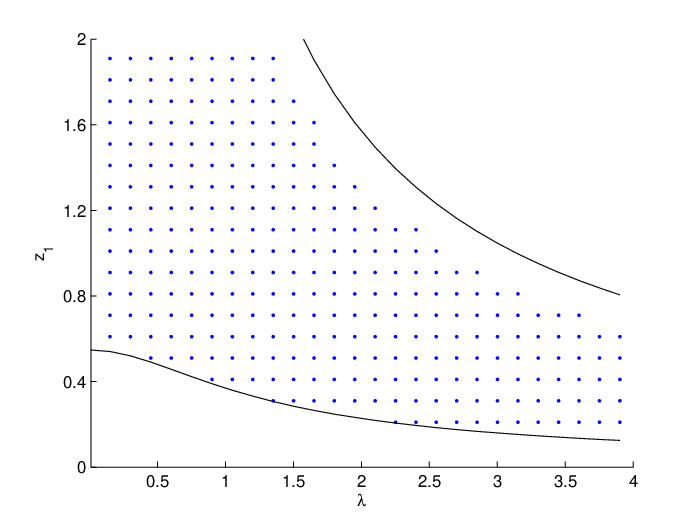 |
| a) sinh solution | b) sine solution |
where
| (3.16) |
Notice that the brane tensions could be positive or negative depending on the parameters involved (, , and ). We may realize that we are living at with an isotropic brane extension along our 4-dimensional space as in (3.4). So the relevant brane tension to us would be: where its sign depends on , and . In figure 2, for one special value of , the positive and negative tension regions are shown for sinh and sine solutions, in plane. The positive and negative regions shrink or expand by changing the value of .
Similar joining process should be considered for field. The Maxwell equation (2.4) indicates that is regular everywhere, on the other hand in (2), field solution admits both plus and minus signs. Thus it should change sign while crossing and . Therefore we take the plus sign for and minus for . Precisely at and we take to be zero. This implies vanishing at where is interpreted as the position of our 4-dimensional universe.
 |
 |
| a | b |
 |
 |
| c | d |
4 Large limit
Let us before studying the noncompact limit by sending to infinity, introduce the proper radius as
| (4.1) |
then the internal 2-dimensional metric reads as
| (4.2) |
where . Using numerical integration of (4.1), the shape of internal space is drawn for various amounts of parameters in figure 3 for the sinh case. Notice that the edges at and are the places of branes. These are almost all possibilities that happen in the sinh case, either in the finite or large limit. In the rest we just concentrate on the sinh case. For sine case the upper limit, , forbids the large limit.
Beside this numerical integration, it is worth to study the behaviors of tensions and radius of the internal space for large limit. Firstly, for brane tensions, the results in the previous section show that the branes at are untouched when is going to infinity. Thus we investigate branes sitting at for very large .
The brane tensions at large are
| (4.3) |
where for large is
| (4.4) |
with and is an independent positive constant. From equations (3.12), we know that is always negative. Thus all tensions goes to infinity at asymptotic distances.
| Finite | Large |
 |
 |
| (a) | (b) |
 |
 |
| (c) | (d) |
 |
 |
| (e) | (f) |
 |
 |
| (g) | (h) |
 |
 |
| a | b |
Now look at (4.4), can be found for large as,
| (4.5) |
Since is negative, as goes to infinity approaches to and for the radius we have,
| (4.6) |
where . Thus as goes to infinity, for negative , diverges and we have a noncompact space, while for nonnegative the radius approaches to zero and a compact space is obtained (see figures 3, 4).
5 Time warp consideration
Let us look at the null energy condition which can be stated as follows[24],
| (5.1) |
where is constructed from energy-momentum tensor as in a d-dimensional space. Then by the Einstein equation it leads to,
| (5.2) |
for any time-like or null vector .
Before checking out this condition in our case, we remind a related no-go theorem in [24], which states that for a class of solutions named ‘time warp’ the null energy condition can not be satisfied for compact extra dimensions. The time warp solutions are introduced as,
| (5.3) |
where denotes the compact coordinates. The above metric covers our solution with and . With this ansatz, the null energy condition gives,
where and are extra directions indices. For one can set using the gauge freedom in coordinate, then,
| (5.5) |
Integrating over the compact extra dimensions implies to be a constant.
Notice that this argument is valid only for . For our metric in (2.3) which is in we find,
| (5.6) |
which can be converted to the form of (5) for with and . We have already chosen a gauge freedom in (2.7) by which we can scape the no-go theorem. Plugging (2.7) in the above inequality one finds the following simple constraint,
| (5.7) |
On the other hand,
| (5.8) | |||||
which is always true (for and case one can send to and zero, respectively, which both satisfy the inequality). This shows that we have constructed a solution which satisfies the energy constraint and escapes the no-go theorem, even in the compact case. There is no contradiction here, since the no-go theorem is valid for and we have a counterexample for .
6 Effective 4-dimensional Planck mass
In the usual extra dimensional theories, effective 4D theory is obtained via integrating over the extra dimensions and interpreting the higher dimensional M-Planck multiplied by the volume of extra dimension as the effective 4D M-Planck. However, the warp factor of time is different from the warp factor of space in here, so we should change the usual procedure.
Let us decompose the 6-dimensional Ricci scalar to the 4-dimensional one in the action as,
| (6.1) | |||||
where is the 6D Ricci scalar, is the determinant of the flat metric of 4D theory, G is the determinant of 6D theory and the 6D Planck-mass is, . We require that:
| (6.2) |
where the integration is over the range of . Now we define the 4D Planck-Mass as:
| (6.3) |
| (6.4) | |||||
| (6.5) | |||||
Equating (6.4) and (6.5) fixes one parameter say ,
| (6.6) |

Notice that our model starts with an asymmetrical spacetime due to the presence of the 3-form field , however at the end by a fine tuning of which is the charge of , one can reach to an effective 4-dimensional symmetric gravity.
7 Conclusion
We have solved the static equations of motion for 6-dimensional Salam-Sezgin model in the presence of 3-form field which provides a 4-dimensional compactification. To find out a global solution over the compact manifold, we consider different patches and join them with the Israel junction conditions which can be satisfied with inserting some branes at the junctions. These conditions also fix some integration constants. More explicitly, we have considered the compact space with angular coordinate , and radial coordinate where the space is defined to be periodic with fundamental region and even under . This gives the torus topology. Then to satisfy the Israel conditions, 3 and 4 branes are inserted at such that they are extended along our 4 dimensional space-time and 4 brane wrapped and 3 branes smeared over the circle. The situation is the same at except that we need to add some 0-branes smeared over the 4 dimensional worldvolume of the 4-brane. We may consider where our brane-universe sits.
We have studied the solution behaviors in different regions of independent parameters and specially for large limit we found that in some cases the internal radius of circle shrinks and changes the topology from torus to sphere.
The asymmetry in space and time is due to the presence of the field. This kind of warping with different time and space warp factors are recently studied in [24] and called ‘time warp’ compactification. It is known that this compactification violates the null energy condition in dimensions [24]. However our compactification which is of course for , shows that the null energy condition is satisfied with a time warp compact space. In section 5, We tried to show why this happens.
Our branes configuration makes it possible to have a 4-dimensional symmetric space at . This can be supplemented with the fact that at . Indeed is discontinuous at this position, and changes the sign while crossing the brane. The mean value of would be zero. There is another view in which the field exponentially vanishing at the other end, , for very large . This enables us to reverse the situation by putting 0-branes at and find a symmetric space-time at for large where vanishes and branes preserve the lorentz symmetry.
Another important issue is introducing an effective 4-dim Planck mass. We have done it by firstly expanding the 6-dimensional gravity action and then integrate out the extra dimensions. Since the solution has two different warp factors for time and space, we encounter with two different integrations. Equating these two integrals we fix the charge of the field and we can factor out integrals over the internal space and find the 4-dimensional Planck mass.
This model is restricted to a static solution, the next development should be a dynamic solution in which all fields would be time dependent. This is consistent with the presence of and would be important if one is interested in finding cosmological application of this model. The stability of this model should be checked and may stabilize some parameters (work in progress).
Acknowledgements
We wish to thank M. Alishahiha, A. Davody, G.W. Gibbons, M. M. Sheikh-Jabbari for useful conversations. Our special thanks are devoted to H. Firouzjahi for really useful discussions and comments in this issue. This work is partially supported by Iranian TWAS at ISMO.
References
- [1] L. Randall and R. Sundrum, “A large mass hierarchy from a small extra dimension,” Phys. Rev. Lett. 83, 3370 (1999) [arXiv:hep-ph/9905221].
- [2] L. Randall and R. Sundrum, “An alternative to compactification,” Phys. Rev. Lett. 83, 4690 (1999) [arXiv:hep-th/9906064].
- [3] H. Nishino and E. Sezgin, “Matter And Gauge Couplings Of N=2 Supergravity In Six-Dimensions,” Phys. Lett. B 144, 187 (1984).
- [4] A. Salam and E. Sezgin, “Chiral Compactification On Minkowski Of N=2 Einstein-Maxwell Supergravity In Six-Dimensions,” Phys. Lett. B 147, 47 (1984).
- [5] S. Randjbar-Daemi, A. Salam, E. Sezgin and J. A. Strathdee, “An Anomaly Free Model In Six-Dimensions,” Phys. Lett. B 151, 351 (1985).
- [6] H. Nishino and E. Sezgin, “The Complete N=2, D = 6 Supergravity With Matter And Yang-Mills Couplings,” Nucl. Phys. B 278, 353 (1986).
- [7] K. i. Maeda and H. Nishino, “Cosmological Solutions In D = 6, N=2 Kaluza-Klein Supergravity: Friedmann Universe Without Fine Tuning,” Phys. Lett. B 154, 358 (1985).
- [8] K. i. Maeda and H. Nishino, “Attractor Universe In Six-Dimensional N=2 Supergravity Kaluza-Klein Theory,” Phys. Lett. B 158, 381 (1985).
- [9] J. J. Halliwell, “CLASSICAL AND QUANTUM COSMOLOGY OF THE SALAM-SEZGIN MODEL,” Nucl. Phys. B 286, 729 (1987).
- [10] E. Papantonopoulos, “Cosmology in six dimensions,” arXiv:gr-qc/0601011.
- [11] M. Cvetic, G. W. Gibbons and C. N. Pope, “A string and M-theory origin for the Salam-Sezgin model,” Nucl. Phys. B 677, 164 (2004) [arXiv:hep-th/0308026].
- [12] S. M. Carroll and M. M. Guica, “Sidestepping the cosmological constant with football-shaped extra dimensions,” arXiv:hep-th/0302067.
- [13] I. Navarro, “Codimension two compactifications and the cosmological constant problem,” JCAP 0309, 004 (2003) [arXiv:hep-th/0302129].
- [14] I. Navarro, “Spheres, deficit angles and the cosmological constant,” Class. Quant. Grav. 20, 3603 (2003) [arXiv:hep-th/0305014].
- [15] Y. Aghababaie, C. P. Burgess, S. L. Parameswaran and F. Quevedo, “Towards a naturally small cosmological constant from branes in 6D supergravity,” Nucl. Phys. B 680, 389 (2004) [arXiv:hep-th/0304256].
- [16] Y. Aghababaie et al., “Warped brane worlds in six dimensional supergravity,” JHEP 0309, 037 (2003) [arXiv:hep-th/0308064].
- [17] G. W. Gibbons, R. Gueven and C. N. Pope, “3-branes and uniqueness of the Salam-Sezgin vacuum,” Phys. Lett. B 595, 498 (2004) [arXiv:hep-th/0307238].
- [18] C. P. Burgess, F. Quevedo, G. Tasinato and I. Zavala, “General axisymmetric solutions and self-tuning in 6D chiral gauged supergravity,” JHEP 0411, 069 (2004) [arXiv:hep-th/0408109].
- [19] H. M. Lee and C. Ludeling, “The general warped solution with conical branes in six-dimensional supergravity,” JHEP 0601, 062 (2006) [arXiv:hep-th/0510026].
- [20] E. J. Copeland and O. Seto, “Dynamical solutions of warped six dimensional supergravity,” JHEP 0708, 001 (2007) [arXiv:0705.4169 [hep-th]].
- [21] A. J. Tolley, C. P. Burgess, C. de Rham and D. Hoover, “Scaling solutions to 6D gauged chiral supergravity,” New J. Phys. 8, 324 (2006) [arXiv:hep-th/0608083].
- [22] C. P. Burgess, C. de Rham, D. Hoover, D. Mason and A. J. Tolley, “Kicking the rugby ball: Perturbations of 6D gauged chiral supergravity,” JCAP 0702, 009 (2007) [arXiv:hep-th/0610078].
- [23] H. M. Lee, “Flux compactifications and supersymmetry breaking in 6D gauged supergravity,” Mod. Phys. Lett. A 24, 165 (2009) [arXiv:0812.3373 [hep-th]].
- [24] S. S. Gubser, “Time warps,” arXiv:0812.5107 [hep-th].
- [25] W. Israel, “Singular hypersurfaces and thin shells in general relativity,” Nuovo Cim. B 44S10 (1966) 1 [Erratum-ibid. B 48 (1967 NUCIA,B44,1.1966) 463].
- [26] C. P. Burgess, D. Hoover, C. de Rham and G. Tasinato, Effective Field Theories and Matching for Codimension-2 Branes,” JHEP 0903, 124 (2009) [arXiv:0812.3820 [hep-th]].
- [27] C. P. Burgess, J. M. Cline, N. R. Constable and H. Firouzjahi, Dynamical stability of six-dimensional warped brane-worlds,” JHEP 0201, 014 (2002) [arXiv:hep-th/0112047].