Calculus on Fractal Curves in $\mathbf{R}^{n}$

• •

  For $a_{0}\leq a<b<c\leq b_{0}$ and $\gamma^{\alpha}(F,a,c)<\infty$

  $$\gamma^{\alpha}(F,a,c)=\gamma^{\alpha}(F,a,b)+\gamma^{\alpha}(F,b,c).$$

• •

  $\gamma^{\alpha}(F,a,b)$ is increasing in $b$ and decreasing in $a$.

• •

  If $\gamma^{\alpha}(F,a,b)$ is finite, $\gamma^{\alpha}(F,a,t)$ is continuous for $t\in[a,b]$.

  Remark: The implication of this result is that no single point has a nonzero mass, or in other words, the mass function is atomless.

• •

  Let $F\subset\mathbf{R}^{n}$ be parametrizable. Let $\lambda$ be a positive real number, $\mathbf{v}\in\mathbf{R}^{n}$, and let $T$ be a rotation operator. We denote

  $$F+\mathbf{v}=\{\mathbf{w}(t)+\mathbf{v}:t\in[a_{0},b_{0}]\}$$

  $$\lambda F=\{\lambda\mathbf{w}(t):t\in[a_{0},b_{0}]\}.$$

  and

  $$TF=\{T\mathbf{w(t)}:t\in[a_{0},b_{0}]\}$$

  Then,

  1. 1.

     Translation :

     $$\gamma^{\alpha}(F+\mathbf{v},a,b)=\gamma^{\alpha}(F,a,b)$$

  2. 2.

     Scaling :

     $$\gamma^{\alpha}(\lambda F,a,b)=\lambda^{\alpha}\gamma^{\alpha}(F,a,b)$$

  3. 3.

     Rotation :

     $$\gamma^{\alpha}(TF,a,b)=\gamma^{\alpha}(F,a,b)$$

The definitions of $\sigma^{\alpha}$, $\gamma^{\alpha}_{\delta}$, and therefore $\gamma^{\alpha}$ implicitly involve the particular parametrization $\mathbf{w}$. Here we show that although defined through the parametrization, these definitions are invariant under the change of parametrization. In order to be able to unambiguously and explicitly refer to the parametrization, we introduce a temporary change in the notation to explicitly indicate dependence on parametrization. Thus given a parametrization $\mathbf{w}:[a,b]\rightarrow\mathbf{R}^{n}$, we use the following notation here:

Let $\mathbf{w}_{1}$ and $\mathbf{w}_{2}$ be two parametrizations of the given fractal curve. By our definition of parametrization, $\mathbf{w}_{1}$ and $\mathbf{w}_{2}$ are continuous and one-to-one. Let the domain of $\mathbf{w}_{1}$ be $[a_{1},b_{1}]$, and that of $\mathbf{w}_{2}$ be $[a_{2},b_{2}]$. We further assume that $\mathbf{w}_{1}$ and $\mathbf{w}_{2}$ have the same orientation, i. e. $\mathbf{w}_{1}(a_{1})=\mathbf{w}_{2}(a_{2})$ and $\mathbf{w}_{1}(b_{1})=\mathbf{w}_{2}(b_{2})$. Thus, $z=\mathbf{w}_{2}^{-1}\circ\mathbf{w}_{1}:[a_{1},b_{1}]\rightarrow[a_{2},b_{2}]$ is a continuous, one-to-one and strictly monotonically increasing function.

Now, given $\delta_{2}>0$ and $\epsilon>0$, there exists a subdivision $P_{2}$ of $[a_{2},b_{2}]$ such that

The set of points $P_{1}=\{z^{-1}(t):t\in P_{2}\}$ forms a subdivision of $[a_{1},b_{1}]$. Then,

by appropriate substitution. Therefore,

which implies that

where $\delta_{1}=|P_{1}|$. Further, since $z$ is continuous, $\lim\delta_{1}=0,\mbox{ as }\delta_{2}\rightarrow 0$, implying that

Since $\epsilon$ is arbitrary, and the same argument remains valid starting with $z^{-1}=\mathbf{w}_{1}^{-1}\circ\mathbf{w}_{2}$, we conclude that

This establishes the fact that the mass function depends only on the fractal curve (i. e. the image of the parametrization), and is independent of the parametrization itself. Since the mass function underlies the calculus developed in the subsequent sections, the calculus is also independent of the particular parametrization chosen.

Now we introduce the integral staircase function for a set $F$ of order $\alpha$.

In the rest of this paper we take $p_{0}=a_{0}$ unless stated otherwise.

Here this function may, more appropriately, be described as a rise function. However we retain the name staircase function because in analogous calculus on fractal subsets of the real line this role is played by a staircase.

Throughout the paper we consider only those sets for which $S_{F}^{\alpha}$ is strictly increasing and thus invertible. Further, we define

which is the function induced by $S_{F}^{\alpha}$ on $F$, and it is also one-to-one.

As an example, figure 1 shows the staircase function for the von koch curve. The curve was parametrized as given in [20].

A log-log graph of the staircase function $S_{F}^{\alpha}(t)$ against the Euclidean distance between origin and $\mathbf{w}(t)$ for the von- koch curve is shown in fig  2.

Let $\alpha$ denote the $\gamma$- dimension of a self similar curve , which is made up of $m$ copies of itself, scaled by a factor of $\frac{1}{n}$ and rotated and translated appropriately. Then using the translation, scaling and rotation properties of the mass function, one can see that the mass of the whole curve is given by

Hence,

This is same as the Hausdorff dimension of self-similar curves [4] .

Thus for self-similar curves

where $dim_{\mathcal{H}}F$ denotes the Hausdorff dimension and $dim_{B}F$ the box dimension of $F$.

For the purpose of this algorithm, $[a,b]$ denotes the domain of $\mathbf{w}$. Further, “randomly” means with a uniform probability unless stated otherwise. The symbol $P$ always indicates the “current” subdivision in consideration.

We begin with a uniform subdivision $P$ such that $|P|=\delta/4$, and iteratively improve it using the following prescription.

1. 1.

   Choose two numbers $x,y\in[a,b]$ randomly, and relabel them if necessary so that $x\leq y$. Then $[x,y]\subset[a,b]$. Let $P^{\prime}=\{t_{i}:0\leq i\leq m\}$ denote the set of all points of $P\cap[x,y]$. We now modify $P^{\prime}$ in one of the following ways with equal probability, and denote the resultant by $P^{\prime\prime}$:

   1. (a)

      With a probability $p_{c}=\min(1,\delta/(y-x))$, we shift each point $t_{i}$ (except $t_{0}$ and $t_{m}$) by a random amount between $[-\delta/2,\delta/2]$, if the resultant subdivision $P^{\prime\prime}$ still satisfies $|P^{\prime\prime}|\leq\delta$.

   2. (b)

      With a probability $p_{d}=\min(1,\delta/(y-x))$, we remove each point $t_{i}$ (except $t_{0}$ and $t_{m}$) from $P^{\prime}$, if the resultant subdivision $P^{\prime\prime}$ still satisfies $|P^{\prime\prime}|\leq\delta$.

   3. (c)

      With a probability $p_{i}=\min(1,\delta/(y-x))$, we insert a point between each $t_{i}$ and $t_{i+1}$ which is chosen randomly from $[t_{i},t_{i+1}]$. (However, to avoid accumulating too much of rounding error, we insert the point only if the distance between $t_{i}$ and $t_{i+1}$ is greater than $\delta/10$.)

2. 2.

   Form a new subdivision $P_{1}=(P\cap[a,x))\cup P^{\prime\prime}\cup(P\cap(y,b])$, i. e. the subdivision of which the points belonging to $[x,y]$ are changed by the above procedure. If $\sigma^{\alpha}[F,P_{1}]<\sigma^{\alpha}[F,P]$, then we consider $P_{1}$ as the “current” subdivision which will be possibly improved further using above steps. Otherwise we consider $P$ again for the purpose.

As the sum $\sigma^{\alpha}[F,P]$ approaches the infimum, many of the newly formed subdivisions $P^{\prime}$ are rejected since they sum up higher than $P$. Thus near the infimum, the sum remains constant for many consecutive iterations, and changes only intermittently. Therefore the usual convergence criterion of terminating iteration when the difference between successive iterations or every $K$ iterations ($K$ being a suitable large integer) goes below certain small number, is not useful in this case. Instead, after examining the sum over a large number of iterations, we observe that the sum stops making significant progress between $N^{\prime}=1000$ to $N^{\prime}=2000$, where $N^{\prime}=N/n$ is the number of iterations $N$ normalized by the current subdivision size $n$. Further, we need to go through all these iterations more than once, just to ensure that subdivision is really optimal. Occasionally it may happen that the sum settles a little above the optimal value, gettting ”trapped” in a ”local minimum”.

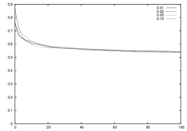
We demonstrate the results of this algorithm as applied on the von Koch curve, parametrized as in equation (1). It turns out that the mass of the entire von Koch curve is a little less than $0.51/\Gamma(\alpha+1)$, $\alpha=\ln(4)/\ln(3)$. The image (under $\mathbf{w}$) of the optimal subdivision found by the algorithm is shown in figure 3, superimposed on the von Koch curve. The evolution of the sum over the normalized number of iterations is shown in figure 4.

The above description assumes that the value of $\alpha$ is the same as the $\gamma$-dimension of the set $F$, say $\alpha_{0}$. We expect $\delta$-independence in the values of $\sigma^{\alpha}[F,P(\delta)]$ where $P(\delta)$ denotes the resultant subdivision of the algorithm at the scale $\delta$, since the value of $\gamma^{\alpha}_{\delta}$ converges to a finite nonzero value. This is what we observe from the values of $\sigma^{\alpha}[F,P(\delta)]$ obtained for various values of $\delta$ (figure 4).

Now we would like to consider cases when $\alpha\neq\alpha_{0}$. Let $0<\delta_{1}<\delta_{2}$. If $\alpha<\alpha_{0}$, then $\gamma^{\alpha}(F,a,b)=\infty$. Therefore we expect that $R(\alpha)=\sigma^{\alpha}[F,P(\delta_{1})]$ $/\sigma^{\alpha}[F,P(\delta_{2})]>1$. Similarly since $\alpha>\alpha_{0}$ implies $\gamma^{\alpha}(F,a,b)=0$, we expect that $R(\alpha)<1$.

This fact can be used to algorithmically calculate the $\gamma$-dimension $\alpha_{0}$: We need to find the number $\alpha_{0}$ such that $R(\alpha_{0})=1$. We already know that $\alpha_{0}\in[1,m],\quad m$ being the embedding dimension, since $F\in\mathbf{R}^{m}$ is a curve. Treating this as the initial bracket of values for $\alpha_{0}$, we just need to use some algorithm such as bisection to shrink this bracket to sufficient accuracy.

Now we introduce limits and continuity along a fractal curve.

We denote the class of bounded functions $f:F\rightarrow R$ by $B(F)$.

Now we define the $F^{\alpha}$-integral

Remark: The $F^{\alpha}$-derivative $D^{\alpha}_{F}(f)$ of a constant function $f:F\rightarrow\mathbf{R}$, $f(\theta)=k\in R$ is zero. This result is to be contrasted with the classical fractional derivative (Riemann-Liouville, and others) of a constant, which is not zero in general [21, 22, 23, 24].

The $F^{\alpha}$-integration and $F^{\alpha}$-differentiation are related as inverse operations of each other. The first fundamental theorem states:

The second fundamental theorem says that the $F^{\alpha}$-integral as a function of upper limit is the inverse of $F^{\alpha}$-derivative except for an additive constant.

The local fractional derivative (LFD) operator constructed in [25] was based on the renormalization of Riemann-Liouville differential operator on the real line. It was utilized to establish the relation between the differentiability properties of nowhere differentiable functions, such as Weierstrass function, and the dimension (Holder exponent) of its graph. The domain of these functions is $\mathbf{R}$ and not a fractal. In [15] though the prescription was developed using LFD, it was realized that to make the local fractional Fokker Planck equation causal and dynamically consistent, the evolution had to be restricted to fractal subsets of the real line. Moreover the order of differentiation had to be the dimension of the fractal support. Since Cantor- like sets are totally disconnected, this necessitated a rigorous development of calculus on fractals from first principles, without using standard fractional calculus on $\mathbf{R}$, which was carried out in [16] The present paper is a logical extension of such a formulation, to fractal curves. While Cantor-like sets considered in [16] are totally disconnected, the von-Koch like fractal curves are continuous but tangentless. Thus all the constructions and proofs have to be carried out keeping in mind this difference of the domain of functions and operators. (Thus for example the notion of ’set of change’ and ’$\alpha$-perfect sets’ was crutial for cantor-like sets in [16] which is repleced by the invertibility of $S_{F}^{\alpha}$ in case of fractal curves considered in this paper.)

There is multiplicity of approaches leading to the notion of local fractional calculus. Various authors [26], [27],[28] have further developed the notion of local fractional differentiation with different approaches. They provide suitable framework for different classes of problems. The development in [26] is based on approach involving difference operators. In finding derivative the quotient is taken with respect to $h^{\alpha}$ where $h$ is an increment of the independent variable. This can be contrasted with the use of $S_{F}^{\alpha}$ in the present approach. This also reflects in the Taylor series where powers of ($S_{F}^{\alpha}$) appear (see equation (17) below) rather than powers of $h$ itself as in [26]. Further the domain is $\mathbf{R}$ in [26] whereas it is a fractal curve in the present paper.

In [27] the notion of classical fractional derivative is modified. Again the essential difference mentioned above for Taylor series and the domain functions is also to be noted here. The development in [28] is based on the Weyl Derivative and the domain of functions is $\mathbf{R}$ and not a fractal curve.

We may emphasize that in the present approach the role of the independent variables is delegated to the staircase/rise function $S_{F}^{\alpha}$, see e.g equation (13). In this sense our approach is like Stieltjes approach in spirit but with some essential differences as noted in [16]. The function $S_{F}^{\alpha}$ captures the essence of fractal support, hence its use makes the calculus suitable for fractals.

References

- [1] Mandelbrot B B 1977 The fractal geometry of nature (Freeman and company).
- [2] A. Bunde and S.Havlin (Eds.), Fractals in Science (Springer, 1995)
- [3] Falconer K 1990 Fractal Geometry: Mathematical foundations and application (John Wiley and Sons).
- [4] Falconer K 1985 The geometry of fractal sets (Cambridge university press).
- [5] Falconer K 1997 Techniques in fractal geormetry(John Wiley and Sons)
- [6] Tricot,C. 1995 Curves and fractal dimensions(Springer- Verlag).
- [7] Edgar G A 1998 Integral,probability and fractal measures(Springer- Verlag,New York).
- [8] Abbott L.F. and Wise.M.B 1981 Dimension of quantum mechanical path Am.J.Phys 49(1) 37.
- [9] Daniel ben-Avraham and Shlomo Havlin Diffusion and Reaction in Fractals and Disordered Systems 2000 Cambridge University Press.
- [10] Adrover A, Schwalm W A, Giona M, Bachand D (1997) Scaling and scaling crossover for transport on anisotropic fractal structures Phys Rev E 55 7304.
- [11] Schwalm W A, Moritz B, Giona M, Schwalm M K (1999) Vector difference calculus for physical lattice models Phys Rev E 59 1217.
- [12] Kigami J, Lapidus M L (1993) Weyl’s Problem for the Spectral Distribution of Laplacians on P.C.F. Self-Similar Fractals Comm Math Phys 158 93.
- [13] Giona M (1999) Contour Integrals and Vector Calculus on Fractal Curves and Interfaces Chaos Solitons and Fractals 10 1349.
- [14] Mendivil F, Vrscay E R (2002) Fractal vector measures and vector calculus on planar fractal domains Chaos Solitons and Fractals 14 1239.
- [15] Kolwankar K M and Gangal A. D 1998 Local fractional Fokker-Planck equation Phys.Rev.Lett. 80 214.
- [16] Abhay Parvate and A.D.Gangal Calculus on fractal subsets of real line -I: formulation Fractals, 17(1), 53-81 (2009).
- [17] Abhay Parvate and A.D.Gangal Calculus on fractal subsets of real line-II :Conjugacy with integer order calculus Pune University pre-print.
- [18] Parvate. A and Gangal A D 2005 Fractal differential equations and fractal-time dynamical systems. Pramana 64 (3), 389.
- [19] Goldberg R R 1970 Methods of real analysis(Oxford and IBH Publishing Co. Pvt.Ltd.)
- [20] L.Nottale and J.Schnieder Fractals and Non-standard Analysis J.Math Phys. 25 (5) May 1984.
- [21] S.G.Samko, A.A. Kilbas and O.I.Marichev, Fractional Integrals and Derivatives- Theory and Applications (Gordon and Breach Science Publshers, 1993).
- [22] R.Hilfer, Applications of Fractional Calculus in Physics (World Scientific Publ.Co., Singapore,2000)
- [23] K.S.Miller and B.Ross, An introduction to the fractional calculus and fractional differential equations (John Wiley, New York 1993)
- [24] Oldham K B and Spanier J 1974 The fractional calculus(Academic Press, New York).
- [25] K.M. Kolwankar and A.D. Gangal Chaos (1996) 505-513.
- [26] Jumarie Computers and Mathematics with Applications (2006) 1367 -1376)
- [27] Ben Adda and Cresson Journal of Mathematical Analysis and Applications (2001) 721737
- [28] Li, Essex and Davison Proceedings of the first Symposium on fractional Derivatives and Their Applications American Society of Mechanical Engineering , Sept.2-6 2003)
- [29] A.Kufner,O.John, S.Fucik, Function Spaces(Noordhoff International Publishing, Leyden, 1977)