跳到论文正文
W Papers独立论文阅读器 arXiv:0906.0652 论文正文 计算阅读时间 · 0%
引用这篇论文根据当前论文元数据生成,正式投稿前建议核对。


License: arXiv.org perpetual non-exclusive license
arXiv:0906.0652v2 [math.ST] 06 Jun 2009

Transductive versions of the LASSO
and the Dantzig Selector

Pierre Alquier    Mohamed Hebiri
Abstract

We consider the linear regression problem, where the number pp of covariates is possibly larger than the number nn of observations (xi,yi)i≤i≤n(x_{i},y_{i})_{i\leq i\leq n}, under sparsity assumptions. On the one hand, several methods have been successfully proposed to perform this task, for example the LASSO in [Tib96] or the Dantzig Selector in [CT07]. On the other hand, consider new values (xi)n+1≤i≤m(x_{i})_{n+1\leq i\leq m}. If one wants to estimate the corresponding yiy_{i}’s, one should think of a specific estimator devoted to this task, referred in [Vap98] as a "transductive" estimator. This estimator may differ from an estimator designed to the more general task "estimate on the whole domain". In this work, we propose a generalized version both of the LASSO and the Dantzig Selector, based on the geometrical remarks about the LASSO in [Alq08, AH08]. The "usual" LASSO and Dantzig Selector, as well as new estimators interpreted as transductive versions of the LASSO, appear as special cases. These estimators are interesting at least from a theoretical point of view: we can give theoretical guarantees for these estimators under hypotheses that are relaxed versions of the hypotheses required in the papers about the "usual" LASSO. These estimators can also be efficiently computed, with results comparable to the ones of the LASSO.

1 Introduction

In many modern applications, a statistician often have to deal with very large datasets. Regression problems may involve a large number of covariates pp, possibly larger than the sample size nn. In this situation, a major issue is dimension reduction, which can be performed through the selection of a small amount of relevant covariates. For this purpose, numerous regression methods have been proposed in the literature, ranging from the classical information criteria such as AIC\mathop{\rm AIC} [Aka73] and BIC\mathop{\rm BIC} [Sch78] to the more recent sparse methods, known as the LASSO [Tib96], and the Dantzig Selector [CT07]. Regularized regression methods have recently witnessed several developments due to the attractive feature of computational feasibility, even for high dimensional data (i.e., when the number of covariates pp is large). We focus on the usual linear regression model:

yi=xiβ∗+εi,i=1,…,n,y_{i}=x_{i}\beta^{*}+\varepsilon_{i},\quad\quad i=1,\ldots,n, (1)

where the design xi=(xi,1,…,xi,p)∈ℝpx_{i}=(x_{i,1},\ldots,x_{i,p})\in\mathbb{R}^{p} is deterministic, β∗=(β1∗,…,βp∗)′∈ℝp\beta^{*}=(\beta^{*}_{1},\ldots,\beta^{*}_{p})^{\prime}\in\mathbb{R}^{p} is the unknown parameter and ε1,…,εn\varepsilon_{1},\ldots,\varepsilon_{n} are i.i.d. centered Gaussian random variables with known variance σ2\sigma^{2}. Let XX denote the matrix with ii-th line equal to xix_{i}, and let XjX_{j} denote its jj-th column, with i∈{1,…,n}i\in\{1,\ldots,n\} and j∈{1,…,p}j\in\{1,\ldots,p\}. So:

X=(x1′,…,xn′)′=(X1,…,Xp).X=(x^{\prime}_{1},\ldots,x^{\prime}_{n})^{\prime}=(X_{1},\ldots,X_{p}).

For the sake of simplicity, we will assume that the observations are normalized in such a way that Xj′​Xj/n=1X_{j}^{\prime}X_{j}/n=1. We denote by YY the vector Y=(y1,…,yn)′Y=(y_{1},\ldots,y_{n})^{\prime}.
For all α≤1\alpha\leq 1 and any vector v∈ℝdv\in\mathds{R}^{d}, we set ∥⋅∥α\|\cdot\|_{\alpha}, the norm: ‖v‖α=(|v1|α+…+|vd|α)1/α\|v\|_{\alpha}=(|v_{1}|^{\alpha}+\ldots+|v_{d}|^{\alpha})^{1/\alpha}. In particular ∥⋅∥2\|\cdot\|_{2} is the euclidean norm. Moreover for all d∈ℕd\in\mathds{N}, we use the notation ‖v‖0=∑i=1d𝟙​(vi≠0).\|v\|_{0}=\sum_{i=1}^{d}\mathds{1}(v_{i}\neq 0).

The problem of estimating the regression parameter in the high dimensional setting have been extensively studied in the statistical literature. Among others, the LASSO [Tib96] (denoted by β^L\hat{\beta}^{L}), the Dantzig Selector [CT07] (denoted by β^D​S\hat{\beta}^{DS}) and the non-negative garrote (in Yuan and Lin [YL07], denoted by β^N​N​G\hat{\beta}^{NNG}) have been proposed to deal with this problem for a large pp, even for p>np>n. These estimators give very good practical results. For instance in [Tib96], simulations and tests on real data have been provided for the LASSO. We also refer to [Kol07, Kol09, MVdGB08, vdG08, DT07, CH08] for related work with different estimators: non-quadratic loss, penalties slightly different from ℓ1\ell_{1} and random design.

From a theoretical point of view, Sparsity Inequalities (SI) have been proved for these estimators under different assumptions. That is upper bounds of order of 𝒪⁡(σ2​‖β∗‖0​log⁡(p)/n)\mathcal{O}\left(\sigma^{2}\|\beta^{*}\|_{0}\log(p)/n\right) for the errors (1/n)​‖X​β^−X​β∗‖22(1/n)\|X\hat{\beta}-X\beta^{*}\|_{2}^{2} and ‖β^−β∗‖22\|\hat{\beta}-\beta^{*}\|_{2}^{2} have been derived, where β^\hat{\beta} is one of the estimators mentioned above. In particular these bounds involve the number of non-zero coordinates in β∗\beta^{*} (multiplied by log⁡(p)\log(p)), instead of dimension pp. Such bounds garanty that under some assumptions, X​β^X\hat{\beta} and β^\hat{\beta} are good estimators of X​β∗X\beta^{*} and β∗\beta^{*} respectively. According to the LASSO β^L\hat{\beta}^{L}, these SI are given for example in [BTW07, BRT07], whereas [CT07, BRT07] provided SI for the Dantzig Selector β^D​S\hat{\beta}^{DS}. On the other hand, Bunea [Bun08] establishes conditions which ensure β^L\hat{\beta}^{L} and β∗\beta^{*} have the same null coordinates. Analog results for β^D​S\hat{\beta}^{DS} can be found in [Lou08].

Now, let us assume that we are given additional observations xi∈ℝpx_{i}\in\mathbb{R}^{p} for n+1≤i≤mn+1\leq i\leq m (with m>nm>n), and introduce the matrix Z=(x1′,…,xm′)′Z=(x^{\prime}_{1},\ldots,x^{\prime}_{m})^{\prime}. Assume that the objective of the statistician is precisely to estimate Z​β∗Z\beta^{*}: namely, he cares about predicting what would be the labels attached to the additional xix_{i}’s. It is argued in [Vap98] that in such a case, a specific estimator devoted to this task should be considered: the transductive estimator. This estimator differs from an estimator tailored for the estimation of β∗\beta^{*} or X​β∗X\beta^{*} like the LASSO. Indeed one usually builds an estimator β^​(X,Y)\hat{\beta}(X,Y) and then computes Z​β^​(X,Y)Z\hat{\beta}(X,Y) to estimate Z​β∗Z\beta^{*}. The approach taken here is to consider estimators β^​(X,Y,Z)\hat{\beta}(X,Y,Z) exploiting the knowledge of ZZ, and then to compute Z​β^​(X,Y,Z)Z\hat{\beta}(X,Y,Z).

Some methods in supervised classification or regression were successfully extended to the transductive setting, such as the well-known Support Vector Machines (SVM) in [Vap98], the Gibbs estimators in [Cat07]. It is argued in the semi-supervised learning literature (see for example [CSZ06] for a recent survey) that taking into account the information on the design given by the new additional xix_{i}’s has a stabilizing effect on the estimator.

In this paper, we study a family of estimators which generalizes the LASSO and the Dantzig Selector. The considered family depends on a q×pq\times p matrix AA, with q∈ℕq\in\mathds{N}, whose choice allows to adapt the estimator to the objective of the statistician. The choice of the matrix AA allows to cover transductive setting.

The rest of paper is organized as follows. In the next section, we motivate the use of the studied family of estimators through geometrical considerations stated in [AH08]. In Sections 3 and 4, we establish Sparsity Inequalities for these estimators. A discussion on the assumptions needed to prove the SI is also provided. In particular, it is shown that the estimators devoted to the transductive setting satisfy these SI with weaker assumptions that those needed by the LASSO or the Dantzig Selector, when m>p>nm>p>n. That is, when the number of news points is large enough. The implementation of our estimators and some numerical experiments are the purpose of Section 5. The results clearly show that the use of a transductive version of the LASSO may improve the performance of the estimation. All proofs of the theoretical results are postponed to Section 7.

2 Preliminaries

In this section we state geometrical considerations (projections on a confidence region) for the LASSO and the Dantzig Selector. These motivate the introduction of our estimators. Finally we discuss the different objectives considered in this paper.

Let us remind that a definition of the LASSO estimate is given by

arg⁡minβ∈ℝp​{‖Y−X​β‖22+2​λ​‖β‖1}.\arg\min_{\beta\in\mathds{R}^{p}}\left\{\left\|Y-X\beta\right\|_{2}^{2}+2\lambda\|\beta\|_{1}\right\}. (2)

A dual form (in [OPT00]) of this program is also of interest:

{arg⁡minβ∈ℝp⁡‖X​β‖22s.t.‖X′​(Y−X​β)‖∞≤λ;\left\{\begin{array}[]{l}\arg\min_{\beta\in\mathds{R}^{p}}\left\|X\beta\right\|_{2}^{2}\\ \\ s.t.\left\|X^{\prime}(Y-X\beta)\right\|_{\infty}\leq\lambda;\end{array}\right. (3)

actually it is proved in [Alq08] that any solution of Program 3 is a solution of Program 2 and that the set {X​β}\{X\beta\} is the same where β\beta is taken among all the solutions of Program 2 or among all the solutions of 3. So both programs are equivalent in terms of estimating X​β∗X\beta^{*}.

Now, let us remind the definition of the Dantzig Selector:

{arg⁡minβ∈ℝp⁡‖β‖1s.t.‖X′​(Y−X​β)‖∞≤λ.\left\{\begin{array}[]{l}\arg\min_{\beta\in\mathds{R}^{p}}\left\|\beta\right\|_{1}\\ \\ s.t.\left\|X^{\prime}(Y-X\beta)\right\|_{\infty}\leq\lambda.\end{array}\right. (4)

Alquier [Alq08] observed that both Programs 3 and 4 can be seen as a projection of the null vector 𝟎𝐩\mathbf{0_{p}} onto the region {β:‖X′​(Y−X​β)‖∞≤λ}\{\beta:\left\|X^{\prime}(Y-X\beta)\right\|_{\infty}\leq\lambda\} that can be interpreted as a confidence region, with confidence 1−η1-\eta, for a given λ\lambda that depends on η\eta (see Lemma 7.1 here for example). The difference between the two programs is the distance (or semi-distance) used for the projection.

Based on these geometrical considerations, we proposed in [AH08] to study the following transductive estimator:

{arg⁡minβ∈ℝp⁡‖Z​β‖22s.t.‖X′​(Y−X​β)‖∞≤λ;\left\{\begin{array}[]{l}\arg\min_{\beta\in\mathds{R}^{p}}\left\|Z\beta\right\|_{2}^{2}\\ \\ s.t.\left\|X^{\prime}(Y-X\beta)\right\|_{\infty}\leq\lambda;\end{array}\right. (5)

that is a projection on the same confidence region, but using a distance adapted to the transductive estimation problem. We proved a Sparsity Inequality for this estimator exploiting a novel sparsity measure.

In this paper, we propose a generalized version of the LASSO and of the Dantzig Selector, based on the same geometrical remark. More precisely for q∈ℕ∗q\in\mathds{N}^{*}, let AA be a q×pq\times p matrix. We propose two general estimators, β^A,λ\hat{\beta}_{A,\lambda} (extension of the LASSO, based on a generalization of Program 2) and β~A,λ\tilde{\beta}_{A,\lambda} (transductive Dantzig Selector, generalization of Program 4). These novel estimators depend on two tuning parameters: λ>0\lambda>0 is a regularization parameter, it plays the same role as the tuning parameter involved in the LASSO, and the matrix AA that will allow to adapt the estimator to the objective of the statistician. More particularly, depending on the choice of the matrix AA, this estimator can be adapted to one of the following objectives:

  • •

    denoising objective: the estimation of X​β∗X\beta^{*}, that is a denoised version of YY. For this purpose, we consider the estimator β^A,λ\hat{\beta}_{A,\lambda}, with A=XA=X. In this case, the estimator will actually be equal to the LASSO β^L\hat{\beta}^{L} and β~A,λ\tilde{\beta}_{A,\lambda}, with the same choice A=XA=X will be equal to the Dantzig Selector;

  • •

    transductive objective: the estimation of Z​β∗Z\beta^{*}, by β^A,λ\hat{\beta}_{A,\lambda} or β~A,λ\tilde{\beta}_{A,\lambda}, with A=n/m​ZA=\sqrt{n/m}Z. We will refer the corresponding estimators as the "Transductive LASSO" and "Transductive Dantzig Selector";

  • •

    estimation objective: the estimation of β∗\beta^{*} itself, by β^A,λ\hat{\beta}_{A,\lambda}, with A=n​IA=\sqrt{n}I. In this case, it appears that both estimators are well defined only in the case p<np<n and are equal to a soft-thresholded version of the usual least-square estimator.

For both estimators and all the above objectives, we prove SI (Sparsity Inequalities). Moreover, we show that these estimators can easily be computed.

3 The "easy case": Ker(X)=Ker(Z)\mathop{\rm Ker}\nolimits(X)=\mathop{\rm Ker}\nolimits(Z)

In this section, we deal with the "easy case", where Ker(A)=Ker(X)\mathop{\rm Ker}\nolimits(A)=\mathop{\rm Ker}\nolimits(X) (think of A=XA=X, A=n​IA=\sqrt{n}I or A=n/m​ZA=\sqrt{n/m}Z). This setting is natural at least in the case p<np<n where both kernels are equal to {0}\{0\} in general. We provide SI (Sparsity Inequality, Theorem 3.3) for the studied estimators, based on the techniques developed in [BRT07].

3.1 Definition of the estimators

Definition 3.1.

For a given parameter λ≥0\lambda\geq 0 and any matrix AA such that K​e​r​(A)=K​e​r​(X)Ker(A)=Ker(X), we consider the estimator given by

β^A,λ∈arg⁡minβ∈ℝp​{−2​Y′​X​(X′​X~)−1​(A′​A)​β+β′​(A′​A)​β+2​λ​‖ΞA​β‖1},\hat{\beta}_{A,\lambda}\in\arg\min_{\beta\in\mathds{R}^{p}}\Bigl\{-2Y^{\prime}X(\widetilde{X^{\prime}X})^{-1}(A^{\prime}A)\beta+\beta^{\prime}(A^{\prime}A)\beta+2\lambda\|\Xi_{A}\beta\|_{1}\Bigr\},

where (X′​X~)−1(\widetilde{X^{\prime}X})^{-1} is exactly (X′​X)−1(X^{\prime}X)^{-1} if (X′​X)(X^{\prime}X) is invertible, and any pseudo-inverse of this matrix otherwise, and where ΞA\Xi_{A} is a diagonal matrix whose (j,j)(j,j)-th coefficient is ξj12​(A)\xi_{j}^{\frac{1}{2}}(A) with ξj​(A)=1n​[(A′​A)​(X′​X~)−1​(A′​A)]j,j\xi_{j}(A)=\frac{1}{n}[(A^{\prime}A)(\widetilde{X^{\prime}X})^{-1}(A^{\prime}A)]_{j,j}.

Remark 3.1.

Equivalently we have

β^A,λ∈arg⁡minβ∈ℝp​{‖Y~A−A​β‖22+2​λ​‖ΞA​β‖1},\hat{\beta}_{A,\lambda}\in\arg\min_{\beta\in\mathds{R}^{p}}\Bigl\{\left\|\tilde{Y}_{A}-A\beta\right\|_{2}^{2}+2\lambda\|\Xi_{A}\beta\|_{1}\Bigr\},

where Y~A=A​(X′​X~)−1​X′​Y\tilde{Y}_{A}=A(\widetilde{X^{\prime}X})^{-1}X^{\prime}Y.

Actually, we are going to consider three particular cases of this estimator in this work, depending on the objective of the statistician:

  • •

    denoising objective: the LASSO, denoted here by β^X,λ\hat{\beta}_{X,\lambda}, given by

    β^X,λ∈arg⁡minβ∈ℝp​{‖Y−X​β‖22+2​λ​‖β‖1}=arg⁡minβ∈ℝp​{−2​Y′​X​β+β′​X′​X​β+2​λ​‖β‖1}\hat{\beta}_{X,\lambda}\in\arg\min_{\beta\in\mathds{R}^{p}}\left\{\left\|Y-X\beta\right\|_{2}^{2}+2\lambda\|\beta\|_{1}\right\}\\ =\arg\min_{\beta\in\mathds{R}^{p}}\left\{-2Y^{\prime}X\beta+\beta^{\prime}X^{\prime}X\beta+2\lambda\|\beta\|_{1}\right\}

    (note that in this case, ΞX=I\Xi_{X}=I since XX is normalized);

  • •

    transductive objective: the Transductive LASSO, denoted here by β^n/m​Z,λ\hat{\beta}_{\sqrt{n/m}Z,\lambda}, given by

    β^nm​Z,λ∈arg⁡minβ∈ℝp​{nm​‖Y~Z−Z​β‖22+2​λ​‖Ξnm​Z′​Z​β‖1};\hat{\beta}_{\sqrt{\frac{n}{m}}Z,\lambda}\in\arg\min_{\beta\in\mathds{R}^{p}}\Bigl\{\frac{n}{m}\left\|\tilde{Y}_{Z}-Z\beta\right\|_{2}^{2}+2\lambda\|\Xi_{\frac{n}{m}Z^{\prime}Z}\beta\|_{1}\Bigr\};
  • •

    estimation objective: β^n​I,λ\hat{\beta}_{\sqrt{n}I,\lambda}, defined by

    β^n​I,λ∈arg⁡minβ∈ℝp​{n​‖Y~I−β‖22+2​λ​‖Ξn​I​β‖1}.\hat{\beta}_{\sqrt{n}I,\lambda}\in\arg\min_{\beta\in\mathds{R}^{p}}\Bigl\{n\left\|\tilde{Y}_{I}-\beta\right\|_{2}^{2}+2\lambda\|\Xi_{\sqrt{n}I}\beta\|_{1}\Bigr\}.

Let us give the analogous definition for an extension of the Dantzig Selector.

Definition 3.2.

For a given parameter λ>0\lambda>0 and any matrix AA such that K​e​r​(A)=K​e​r​(X)Ker(A)=Ker(X), we consider the estimator given by

β~A,λ={arg⁡minβ∈ℝp⁡‖β‖1s.t.‖ΞA−1​A′​A​((X′​X~)−1​X′​Y−β)‖∞≤λ.\tilde{\beta}_{A,\lambda}=\left\{\begin{array}[]{l}\arg\min_{\beta\in\mathds{R}^{p}}\left\|\beta\right\|_{1}\\ \\ s.t.\left\|\Xi_{A}^{-1}A^{\prime}A((\widetilde{X^{\prime}X})^{-1}X^{\prime}Y-\beta)\right\|_{\infty}\leq\lambda.\end{array}\right. (6)

Here again, we are going to consider three cases, for A=XA=X, A=n/m​ZA=\sqrt{n/m}Z and A=n​IA=\sqrt{n}I, and it is easy to check that for A=XA=X we have exactly the usual definition of the Dantzig Selector (Program 4). Moreover, here again, note that we can rewrite this estimator:

β~A,λ={arg⁡minβ∈ℝp⁡‖β‖1s.t.‖ΞA−1​A′​(Y~A−A​β)‖∞≤λ.\tilde{\beta}_{A,\lambda}=\left\{\begin{array}[]{l}\arg\min_{\beta\in\mathds{R}^{p}}\left\|\beta\right\|_{1}\\ \\ s.t.\left\|\Xi_{A}^{-1}A^{\prime}(\tilde{Y}_{A}-A\beta)\right\|_{\infty}\leq\lambda.\end{array}\right.

The following proposition provides an interpretation of our estimators when A=n​IA=\sqrt{n}I.

Proposition 3.1.

Let us assume that (X′​X)(X^{\prime}X) is invertible. Then β^n​I,λ=β~n​I,λ\hat{\beta}_{\sqrt{n}I,\lambda}=\tilde{\beta}_{\sqrt{n}I,\lambda} and this is a soft-thresholded least-square estimator: let us put β^L​S​E=(X′​X)−1​X′​Y\hat{\beta}^{LSE}=(X^{\prime}X)^{-1}X^{\prime}Y then β^n​I,λ\hat{\beta}_{\sqrt{n}I,\lambda} is the vector obtained by replacing the jj-th coordinate bj=β^jL​S​Eb_{j}=\hat{\beta}^{LSE}_{j} of β^L​S​E\hat{\beta}^{LSE} by s​g​n​(bj)​(|bj|−λ​ξj​(n​I)/n)+sgn(b_{j})\left(|b_{j}|-\lambda\xi_{j}(nI)/n\right)_{+}, where we use the standard notation s​g​n​(x)=+1sgn(x)=+1 if x≥0x\geq 0, s​g​n​(x)=−1sgn(x)=-1 if x<0x<0 and (x)+=max⁡(x,0)(x)_{+}=\max(x,0).

Proposition 3.2 deals with a dual definition of the estimator β^A,λ\hat{\beta}_{A,\lambda}.

Proposition 3.2.

When Ker(A)=Ker(X)\mathop{\rm Ker}\nolimits(A)=\mathop{\rm Ker}\nolimits(X), the solutions β\beta of the following program:

{arg⁡minβ∈ℝp⁡‖A​β‖22s.t.‖ΞA−1A′((Y~A−Aβ)‖∞≤λ\left\{\begin{array}[]{l}\arg\min_{\beta\in\mathds{R}^{p}}\left\|A\beta\right\|_{2}^{2}\\ \\ s.t.\left\|\Xi_{A}^{-1}A^{\prime}((\tilde{Y}_{A}-A\beta)\right\|_{\infty}\leq\lambda\end{array}\right.

all satisfy X​β=X​β^A,λX\beta=X\hat{\beta}_{A,\lambda} and A​β=A​β^A,λA\beta=A\hat{\beta}_{A,\lambda}.

Proofs can be found in Section 7, page 7.

3.2 Theoretical results

Let us first introduce our main assumption. This assumption is stated with a given p×pp\times p matrix MM and a given real number x>0x>0.

Assumption H⁡(M,x)H(M,x):

there is a constant c⁡(M)>0c(M)>0 such that, for any α∈ℝp\alpha\in\mathds{R}^{p} such that ∑j:βj∗=0ξj(M)|αj|≤x∑j:βj∗≠0ξj(M)|αj|\sum_{j:\beta^{*}_{j}=0}\xi_{j}(M)\left|\alpha_{j}\right|\leq x\sum_{j:\beta^{*}_{j}\neq 0}\xi_{j}(M)\left|\alpha_{j}\right| we have

α′Mα≥c(M)n∑j:βj∗≠0αj2.\alpha^{\prime}M\alpha\geq c(M)n\sum_{j:\beta_{j}^{*}\neq 0}\alpha_{j}^{2}. (7)

First, let us explain briefly the meaning of this hypothesis. In the case, where MM is invertible, the condition

α′Mα≥c(M)n∑j:βj∗≠0αj2\alpha^{\prime}M\alpha\geq c(M)n\sum_{j:\beta_{j}^{*}\neq 0}\alpha_{j}^{2}

is always satisfied for any α∈ℝp\alpha\in\mathds{R}^{p} with c⁡(M)c(M) larger than the smallest eigenvalue of M/nM/n. However, for the LASSO, we have M=(X′​X)M=(X^{\prime}X) and MM cannot be invertible if p>np>n. Even in this case, Assumption H⁡(M,x)H(M,x) may still be satisfied. Indeed, the assumption requires that Inequality (7) holds only for a small for a small subset of ℝp\mathds{R}^{p} determined by the condition ∑j:βj∗=0ξj(M)|αj|≤x∑j:βj∗≠0ξj(M)|αj|.\sum_{j:\beta^{*}_{j}=0}\xi_{j}(M)\left|\alpha_{j}\right|\leq x\sum_{j:\beta^{*}_{j}\neq 0}\xi_{j}(M)\left|\alpha_{j}\right|. For M=(X′​X)M=(X^{\prime}X), this assumption becomes exactly the one taken in [BTW07]. In that paper, the necessity of such an hypothesis is also discussed.

Theorem 3.3.

Let us assume that Assumption H⁡(A′​A,3)H(A^{\prime}A,3) is satisfied and that K​e​r​(A)=K​e​r​(X)Ker(A)=Ker(X). Let us choose 0<η<10<\eta<1 and λ=2​σ​2​n​log⁡(p/η)\lambda=2\sigma\sqrt{2n\log\left(p/\eta\right)}. With probability at least 1−η1-\eta on the draw of YY, we have simultaneously

‖A(β^A,λ−β∗)‖22≤72​σ2c⁡(A′​A)log(pη)∑j:βj∗≠0ξj(A),\left\|A\left(\hat{\beta}_{A,\lambda}-\beta^{*}\right)\right\|_{2}^{2}\leq\frac{72\sigma^{2}}{c(A^{\prime}A)}\log\left(\frac{p}{\eta}\right)\sum_{j:\beta^{*}_{j}\neq 0}\xi_{j}(A),

and

‖ΞA(β^A,λ−β∗)‖1≤24​2​σc⁡(A′​A)(log⁡(p/η)n)12∑j:βj∗≠0ξj(A).\left\|\Xi_{A}\left(\hat{\beta}_{A,\lambda}-\beta^{*}\right)\right\|_{1}\leq\frac{24\sqrt{2}\sigma}{c(A^{\prime}A)}\left(\frac{\log\left(p/\eta\right)}{n}\right)^{\frac{1}{2}}\sum_{j:\beta^{*}_{j}\neq 0}\xi_{j}(A).

In particular, the first inequality gives

  • •

    if Assumption H⁡(X′​X,3)H(X^{\prime}X,3) is satisfied, with probability at least 1−η1-\eta,

    1n​‖X⁡(β^X,λ−β∗)‖22≤72​σ2n​c​(X′​X)​‖β∗‖0​log⁡(pη);\frac{1}{n}\left\|X\left(\hat{\beta}_{X,\lambda}-\beta^{*}\right)\right\|_{2}^{2}\leq\frac{72\sigma^{2}}{nc(X^{\prime}X)}\|\beta^{*}\|_{0}\log\left(\frac{p}{\eta}\right);
  • •

    if Assumption H⁡(nm​Z′​Z,3)H(\frac{n}{m}Z^{\prime}Z,3) is satisfied, and if K​e​r​(Z)=K​e​r​(X)Ker(Z)=Ker(X), with probability at least 1−η1-\eta,

    1m‖Z(β^Z,λ−β∗)‖22≤72​σ2n​c​(nm​Z′​Z)∑j:βj∗≠0ξj(n/mZ)log(pη);\frac{1}{m}\left\|Z\left(\hat{\beta}_{Z,\lambda}-\beta^{*}\right)\right\|_{2}^{2}\leq\frac{72\sigma^{2}}{nc(\frac{n}{m}Z^{\prime}Z)}\sum_{j:\beta_{j}^{*}\neq 0}\xi_{j}\left(\sqrt{n/m}Z\right)\log\left(\frac{p}{\eta}\right);
  • •

    and if (X′​X)(X^{\prime}X) is invertible, with probability at least 1−η1-\eta,

    ‖β^n​I,λ−β∗‖22≤72​σ2n​c​(n​I)∑j:βj∗≠0ξj(nI)log(pη).\left\|\hat{\beta}_{\sqrt{n}I,\lambda}-\beta^{*}\right\|_{2}^{2}\leq\frac{72\sigma^{2}}{nc(nI)}\sum_{j:\beta_{j}^{*}\neq 0}\xi_{j}(nI)\log\left(\frac{p}{\eta}\right).

This result shows that each of these three estimators satisfy at least a SI for the task it is designed for. For example, the LASSO is proved to have "good" performance for the estimation of X​β∗X\beta^{*} and the Transductive LASSO is proved to have good performance for the estimation of Z​β∗Z\beta^{*}. However we cannot assert that, for example, the LASSO performs better than the Transductive LASSO for the estimation of Z​β∗Z\beta^{*}.

Remark 3.2.

For A=XA=X, the particular case of our result applied to the LASSO is quite similar to the result given in [BTW07] on the LASSO. Actually, Theorem 3.3 can be seen as a generalization of the result in [BTW07] and it should be noted that the proof used to prove Theorem 3.3 uses arguments introduced in [BTW07].

Remark 3.3.

As soon as A′​AA^{\prime}A is better determined than X′​XX^{\prime}X, Assumption H⁡(A,x)H(A,x) is less restrictive than H⁡(X′​X,x)H(X^{\prime}X,x). In particular, in the case where m>nm>n, Assumption H⁡((n/m)​Z′​Z,x)H((n/m)Z^{\prime}Z,x) is expected to be less restrictive than Assumption H⁡(X′​X,x)H(X^{\prime}X,x).

Now we give the analogous result for the estimator β~A,λ\tilde{\beta}_{A,\lambda}.

Theorem 3.4.

Let us assume that Assumption H⁡(A′​A,1)H(A^{\prime}A,1) is satisfied and that K​e​r​(A)=K​e​r​(X)Ker(A)=Ker(X). Let us choose 0<η<10<\eta<1 and λ=2​σ​2​n​log⁡(p/η)\lambda=2\sigma\sqrt{2n\log\left(p/\eta\right)}. With probability at least 1−η1-\eta on the draw of YY, we have simultaneously

‖A(β~A,λ−β∗)‖22≤72​σ2c⁡(A′​A)log(pη)∑j:βj∗≠0ξj(A),\left\|A\left(\tilde{\beta}_{A,\lambda}-\beta^{*}\right)\right\|_{2}^{2}\leq\frac{72\sigma^{2}}{c(A^{\prime}A)}\log\left(\frac{p}{\eta}\right)\sum_{j:\beta^{*}_{j}\neq 0}\xi_{j}(A),

and

‖ΞA(β~A,λ−β∗)‖1≤12​2​σc⁡(A′​A)(log⁡(p/η)n)12∑j:βj∗≠0ξj(A).\left\|\Xi_{A}\left(\tilde{\beta}_{A,\lambda}-\beta^{*}\right)\right\|_{1}\leq\frac{12\sqrt{2}\sigma}{c(A^{\prime}A)}\left(\frac{\log\left(p/\eta\right)}{n}\right)^{\frac{1}{2}}\sum_{j:\beta^{*}_{j}\neq 0}\xi_{j}(A).

4 An extension to the general case

In this section, we only deal with the transductive setting, A=n/m​ZA=\sqrt{n/m}Z. Let us remind that in such a framework, we observe XX which consists of some observations xix_{i} associated to labels YiY_{i} in YY, for i∈{1,…,n}i\in\{1,\ldots,n\}. Moreover we have additional observations xix_{i} for i∈{n+1,…,m}i\in\{n+1,\ldots,m\} with m>nm>n. We also recall that ZZ contains all the xix_{i} for i∈{1,…,m}i\in\{1,\ldots,m\} and that the objective is to estimate the corresponding labels YiY_{i}, let us put Y~=(Y1,…,Ym)′\tilde{Y}=(Y_{1},\ldots,Y_{m})^{\prime}.

4.1 General remarks

Let us have look at the definition of β^n/m​Z,λ\hat{\beta}_{\sqrt{n/m}Z,\lambda}, for example as given in Remark 3.1:

β^nm​Z,λ∈arg⁡minβ∈ℝp​{nm​‖Y~Z−Z​β‖22+2​λ​‖Ξnm​Z′​Z​β‖1},\hat{\beta}_{\sqrt{\frac{n}{m}}Z,\lambda}\in\arg\min_{\beta\in\mathds{R}^{p}}\Bigl\{\frac{n}{m}\left\|\tilde{Y}_{Z}-Z\beta\right\|_{2}^{2}+2\lambda\|\Xi_{\frac{n}{m}Z^{\prime}Z}\beta\|_{1}\Bigr\},

where actually Y~Z=Z​(X′​X~)−1​X​Y\tilde{Y}_{Z}=Z\left(\widetilde{X^{\prime}X}\right)^{-1}XY can be interpreted as a preliminary estimator of Y~\tilde{Y}. Hence, in any case, we propose the following procedure.
Let us assume that, depending on the context, the user has a natural (and not necessary efficient) estimator of Y~=(Y1,…,Yn+m)′\tilde{Y}=(Y_{1},\ldots,Y_{n+m})^{\prime}. Note this estimator Yˇ\check{Y}.

Definition 4.1.

The Transductive LASSO is given by:

β^Yˇ,nm​Z,λ∈arg⁡minβ∈ℝp​{nm​‖Yˇ−Z​β‖22+2​λ​‖Ξnm​Z′​Z​β‖1},\hat{\beta}_{\check{Y},\sqrt{\frac{n}{m}}Z,\lambda}\in\arg\min_{\beta\in\mathds{R}^{p}}\Bigl\{\frac{n}{m}\left\|\check{Y}-Z\beta\right\|_{2}^{2}+2\lambda\|\Xi_{\frac{n}{m}Z^{\prime}Z}\beta\|_{1}\Bigr\},

and the Transductive Dantzig Selector is defined as:

β~Yˇ,nm​Z,λ={arg⁡minβ∈ℝp⁡‖β‖1s.t.‖nm​Ξn/m​Z−1​Z′​(Yˇ−Z​β)‖∞≤λ.\tilde{\beta}_{\check{Y},\sqrt{\frac{n}{m}}Z,\lambda}=\left\{\begin{array}[]{l}\arg\min_{\beta\in\mathds{R}^{p}}\left\|\beta\right\|_{1}\\ \\ s.t.\left\|\frac{n}{m}\Xi_{\sqrt{n/m}Z}^{-1}Z^{\prime}(\check{Y}-Z\beta)\right\|_{\infty}\leq\lambda.\end{array}\right.

In the next subsection, we propose a context where we have a natural estimator Yˇ\check{Y} and give a SI on this estimator.

4.2 An example: small labeled dataset, large unlabeled dataset

The idea of this example is to consider the case where the examples xix_{i} for 1≤i≤n1\leq i\leq n are "representative" of the large populations xix_{i} for 1≤i≤m1\leq i\leq m.

Consider, Z=(x1′,…,xm′)′Z=(x_{1}^{\prime},\ldots,x_{m}^{\prime})^{\prime} where the xi′​sx_{i}^{\prime}s are the points of interest: we want to estimate Y~=Z​β∗\tilde{Y}=Z\beta^{*}. However, we just have a very expensive and noisy procedure, that, given a point xix_{i}, returns Yi=xi​β∗+εiY_{i}=x_{i}\beta^{*}+\varepsilon_{i}, where the εi\varepsilon_{i}’s are 𝒩⁡(0,σ2)\mathcal{N}(0,\sigma^{2}) independent random variables. In such a case, the procedure cannot be applied for the whole dataset Z=(x1′,…,xm′)′Z=(x_{1}^{\prime},\ldots,x_{m}^{\prime})^{\prime}. We can only make a deal with a "representative" sample of size nn. A typical case could be n<p<mn<p<m.

First, let us introduce a slight modification of our main hypothesis. It is also stated with a given p×pp\times p matrix MM and a given real number x>0x>0.

Assumption H′​(M,x)H^{\prime}(M,x):

there is a c⁡(M)>0c(M)>0 such that, for any α∈ℝp\alpha\in\mathds{R}^{p} such that ∑j:βj∗=0|αj|≤x∑j:βj∗≠0|αj|\sum_{j:\beta^{*}_{j}=0}\left|\alpha_{j}\right|\leq x\sum_{j:\beta^{*}_{j}\neq 0}\left|\alpha_{j}\right| we have

α′Mα≥c(M)n∑j:βj∗≠0αj2.\alpha^{\prime}M\alpha\geq c(M)n\sum_{j:\beta^{*}_{j}\neq 0}\alpha_{j}^{2}.

We can now state our main result.

Theorem 4.1.

Let us assume that Assumption H′​((n/m)​Z′​Z,1)H^{\prime}((n/m)Z^{\prime}Z,1) is satisfied. Let us choose 0<η<10<\eta<1 and λ1=λ2=10−1​σ​2​n​log⁡(p/η)\lambda_{1}=\lambda_{2}=10^{-1}\sigma\sqrt{2n\log\left(p/\eta\right)}. Moreover, let us assume that

∀u∈ℝp​ with ​‖u‖1≤‖β∗‖1,‖((X′​X)−nm​(Z′​Z))​u‖∞<σ10​2​n​log⁡(pη).\forall u\in\mathds{R}^{p}\text{ with }\|u\|_{1}\leq\|\beta^{*}\|_{1},\quad\left\|\left((X^{\prime}X)-\frac{n}{m}(Z^{\prime}Z)\right)u\right\|_{\infty}<\frac{\sigma}{10}\sqrt{2n\log\left(\frac{p}{\eta}\right)}. (8)

Let Yˇλ1=Z​β~X,λ1\check{Y}_{\lambda_{1}}=Z\tilde{\beta}_{X,\lambda_{1}} be a preliminary estimator of Y~\tilde{Y}, based on ths Dantzig Selector given by (6) (with A=XA=X). Then define the Transductive LASSO by

β^nm​Z,20​λ2∗={arg⁡minβ∈ℝp​nm​‖Z​β‖22s.t.‖nm​Z′​(Yˇλ1−Z​β)‖∞≤20​λ2,\hat{\beta}^{*}_{\frac{n}{m}Z,20\lambda_{2}}=\left\{\begin{array}[]{l}\arg\min_{\beta\in\mathds{R}^{p}}\frac{n}{m}\left\|Z\beta\right\|_{2}^{2}\\ \\ s.t.\left\|\frac{n}{m}Z^{\prime}(\check{Y}_{\lambda_{1}}-Z\beta)\right\|_{\infty}\leq 20\lambda_{2},\end{array}\right.

and the Transductive Dantzig Selector

β~nm​Z,λ2∗={arg⁡minβ∈ℝp⁡‖β‖1s.t.‖nm​Z′​(Yˇλ1−Z​β)‖∞≤λ2.\tilde{\beta}^{*}_{\frac{n}{m}Z,\lambda_{2}}=\left\{\begin{array}[]{l}\arg\min_{\beta\in\mathds{R}^{p}}\left\|\beta\right\|_{1}\\ \\ s.t.\left\|\frac{n}{m}Z^{\prime}(\check{Y}_{\lambda_{1}}-Z\beta)\right\|_{\infty}\leq\lambda_{2}.\end{array}\right.

With probability at least 1−η1-\eta on the draw of YY, we have simultaneously

1m​‖Z⁡(β~nm​Z,λ2∗−β∗)‖22≤16​σ2n​c​((n/m)​Z′​Z)​log⁡(pη)​‖β∗‖0,\frac{1}{m}\left\|Z(\tilde{\beta}^{*}_{\frac{n}{m}Z,\lambda_{2}}-\beta^{*})\right\|_{2}^{2}\leq\frac{16\sigma^{2}}{nc((n/m)Z^{\prime}Z)}\log\left(\frac{p}{\eta}\right)\|\beta^{*}\|_{0},
‖β~nm​Z,λ2∗−β∗‖1≤8​σc⁡((n/m)​Z′​Z)​(log⁡(p/η)n)12​‖β∗‖0,\left\|\tilde{\beta}^{*}_{\frac{n}{m}Z,\lambda_{2}}-\beta^{*}\right\|_{1}\leq\frac{8\sigma}{c((n/m)Z^{\prime}Z)}\left(\frac{\log\left(p/\eta\right)}{n}\right)^{\frac{1}{2}}\|\beta^{*}\|_{0},

and moreover, if H′​((n/m)​Z′​Z,5)H^{\prime}((n/m)Z^{\prime}Z,5) is also satisfied,

1m​‖Z⁡(β^nm​Z,20​λ2∗−β∗)‖22≤88​σ2n​c​((n/m)​Z′​Z)​log⁡(pη)​‖β∗‖0,\frac{1}{m}\left\|Z(\hat{\beta}^{*}_{\frac{n}{m}Z,20\lambda_{2}}-\beta^{*})\right\|_{2}^{2}\leq\frac{88\sigma^{2}}{nc((n/m)Z^{\prime}Z)}\log\left(\frac{p}{\eta}\right)\|\beta^{*}\|_{0},
‖β^nm​Z,20​λ2∗−β∗‖1≤54​σc⁡((n/m)​Z′​Z)​(log⁡(p/η)n)12​‖β∗‖0.\left\|\hat{\beta}^{*}_{\frac{n}{m}Z,20\lambda_{2}}-\beta^{*}\right\|_{1}\leq\frac{54\sigma}{c((n/m)Z^{\prime}Z)}\left(\frac{\log\left(p/\eta\right)}{n}\right)^{\frac{1}{2}}\|\beta^{*}\|_{0}.

First, let us remark that the preliminary estimator Yˇλ1\check{Y}_{\lambda_{1}} is defined using the Dantzig Selector β~X,λ1\tilde{\beta}_{X,\lambda_{1}}. We could give exactly the same kind of results using a the LASSO β^X,λ1\hat{\beta}_{X,\lambda_{1}} as a preliminary estimator.

Now, let us give a look at the new hypothesis, Inequality (8). We can interpret this condition as the fact that the xix_{i}’s for 1≤i≤n1\leq i\leq n are effectively representative of the wide population: so X′​X/nX^{\prime}X/n is "not too far" from Z′​Z/mZ^{\prime}Z/m. We will end this section by a result that proves that this is effectively the case in a typical situation.

Proposition 4.2.

Assume that m=k​nm=kn for an integer value k∈ℕ∖{0,1}k\in\mathds{N}\setminus\{0,1\}. Let us assume that XX and ZZ are build in the following way: we have a population χ1=(χ1,1,…,χ1,p)∈ℝp\chi_{1}=(\chi_{1,1},\ldots,\chi_{1,p})\in\mathds{R}^{p},…, χm∈ℝp\chi_{m}\in\mathds{R}^{p} (the points of interest). Then, we draw uniformly without replacement, nn of the χi\chi_{i}’s to be put in XX: more formally, but equivalently, we draw uniformly a permutation σ\sigma of {1,…,m}\{1,\ldots,m\} and we put X=(x1′,…,xn′)′=(χσ⁡(1)′,…,χσ⁡(n)′)′X=(x_{1}^{\prime},\ldots,x_{n}^{\prime})^{\prime}=(\chi_{\sigma(1)}^{\prime},\ldots,\chi_{\sigma(n)}^{\prime})^{\prime} and Z=(x1′,…,xm′)′=(χσ⁡(1)′,…,χσ⁡(m)′)′Z=(x_{1}^{\prime},\ldots,x_{m}^{\prime})^{\prime}=(\chi_{\sigma(1)}^{\prime},\ldots,\chi_{\sigma(m)}^{\prime})^{\prime}.
Let us assume that for any (i,j)∈{1,…,m}×{1,…,p}(i,j)\in\{1,\ldots,m\}\times\{1,\ldots,p\}, χi,j2<κ\chi_{i,j}^{2}<\kappa for some κ>0\kappa>0, and that p≥2p\geq 2. Then, with probability at least 1−η1-\eta, for any u∈ℝpu\in\mathds{R}^{p},

‖(X′​X−nm​Z′​Z)​u‖∞≤‖u‖1​2​κ​kk−1​2​log⁡pη.\left\|\left(X^{\prime}X-\frac{n}{m}Z^{\prime}Z\right)u\right\|_{\infty}\leq\left\|u\right\|_{1}\frac{2\kappa k}{k-1}\sqrt{2\log\frac{p}{\eta}}.

In particular, if we have

‖u‖1≤‖β∗‖1​ and ​κ≤k−110​k​σ‖β∗‖1\|u\|_{1}\leq\|\beta^{*}\|_{1}\text{ and }\kappa\leq\frac{k-1}{10\,k}\frac{\sigma}{\|\beta^{*}\|_{1}}

then we have

‖(X′​X−nm​Z′​Z)​u‖∞≤σ​2​n​log⁡(pη).\left\|\left(X^{\prime}X-\frac{n}{m}Z^{\prime}Z\right)u\right\|_{\infty}\leq\sigma\sqrt{2n\log\left(\frac{p}{\eta}\right)}.

Let us just mention that the assumption m=k​nm=kn is not restrictive. It has been introduced for the sake of simplicity.

5 Experimental results

Implementation. Since the paper of Tibshirani [Tib96], several effective algorithms to compute the LASSO have been proposed and studied (for instance Interior Points methods [KKL+07], LARS [EHJT04], Pathwise Coordinate Optimization [FHHT07], Relaxed Greedy Algorithms [HCB08]). For the Dantzig Selector, a linear method was proposed in the first paper [CT07]. The LARS algorithm was also successfully extended in [JRL09] to compute the Dantzig Selector.
Then there are many algorithms to compute β^A,λ\hat{\beta}_{A,\lambda} and β~A,λ\tilde{\beta}_{A,\lambda}, when A=XA=X. Thanks to Proposition 3.1, it is also clear that we can easily find an efficient algorithm for the case A=n​IA=\sqrt{n}I.
The general form of the estimators β^A,λ\hat{\beta}_{A,\lambda} and β~A,λ\tilde{\beta}_{A,\lambda} given by Definitions 3.1 and 3.2, allows to use one of the algorithms mentioned previously to compute our estimator in two cases. For example, from Remark 3.1, we have:

β^A,λ∈arg⁡minβ∈ℝp​{‖Y~A−A​β‖22+2​λ​‖ΞA​β‖1},\hat{\beta}_{A,\lambda}\in\arg\min_{\beta\in\mathds{R}^{p}}\Bigl\{\left\|\tilde{Y}_{A}-A\beta\right\|_{2}^{2}+2\lambda\|\Xi_{A}\beta\|_{1}\Bigr\},

then we just have to compute Y~A\tilde{Y}_{A}, to put B=A​ΞA−1B=A\Xi_{A}^{-1}, to use any program that computes the LASSO to determine

γ^∈arg⁡minγ∈ℝp​{‖Y~A−B​γ‖22+2​λ​‖γ‖1}\hat{\gamma}\in\arg\min_{\gamma\in\mathds{R}^{p}}\Bigl\{\left\|\tilde{Y}_{A}-B\gamma\right\|_{2}^{2}+2\lambda\|\gamma\|_{1}\Bigr\}

and then to put β^A,λ=ΞA−1​γ\hat{\beta}_{A,\lambda}=\Xi_{A}^{-1}\gamma.

In the rest of this section, we compare the LASSO and the transductive LASSO on the classical toy example introduced by Tibshirani [Tib96] and used as a benchmark.

Data description. In the model proposed by Tibshirani, we have

Yi=xi​β∗+εiY_{i}=x_{i}\beta^{*}+\varepsilon_{i}

for i∈{1,…,n}i\in\{1,\ldots,n\}, β∗∈ℝp\beta^{*}\in\mathds{R}^{p} and the εi\varepsilon_{i} are i.i.d. 𝒩⁡(0,σ2)\mathcal{N}(0,\sigma^{2}). Finally, the (xi)i∈{1,…,m}(x_{i})_{i\in\{1,\ldots,m\}} are generated from a probability distribution: they are independent and identically distributed

xi∼𝒩⁡((0⋮0),(1ρ……ρp−1ρ1ρ…ρp−2⋮⋱⋱⋱⋮ρp−2…ρ1ρρp−1……ρ1)),x_{i}\sim\mathcal{N}\left(\left(\begin{array}[]{c}0\\ \vdots\\ 0\end{array}\right),\left(\begin{array}[]{c c c c c}1&\rho&\dots&\dots&\rho^{p-1}\\ \rho&1&\rho&\dots&\rho^{p-2}\\ \vdots&\ddots&\ddots&\ddots&\vdots\\ \rho^{p-2}&\dots&\rho&1&\rho\\ \rho^{p-1}&\dots&\dots&\rho&1\end{array}\right)\right),

for a given ρ∈]−1,1[\rho\in]-1,1[.

As in [Tib96], we set p=8p=8. In a first experiment, we take (n,m)=(7,10)(n,m)=(7,10), ρ=0.5\rho=0.5, σ=1\sigma=1 and β∗=(3,1.5,0,0,2,0,0,0)\beta^{*}=(3,1.5,0,0,2,0,0,0) ("sparse"). Then, in order to check the robustness of the results, we consider successively ρ=0.5\rho=0.5 by ρ=0.9\rho=0.9 (correlated variables), σ=1\sigma=1 by σ=3\sigma=3 (noisy case), β∗=(3,1.5,0,0,2,0,0,0)\beta^{*}=(3,1.5,0,0,2,0,0,0) by β∗=(5,0,0,0,0,0,0,0)\beta^{*}=(5,0,0,0,0,0,0,0) ("very sparse" case), (n,m)=(7,10)(n,m)=(7,10) by (n,m)=(7,20)(n,m)=(7,20) (larger unlabeled set), (n,m)=(20,30)(n,m)=(20,30) (p<np<n, easy case) and finally (n,m)=(20,120)(n,m)=(20,120).

We use the version of the Transductive LASSO proposed in Section 4: for a given λ1\lambda_{1}, we first compute the LASSO estimator β^X,λ1\hat{\beta}_{X,\lambda_{1}}. In the sequel, the Transductive LASSO is given by

β^T​L​(λ1,λ2)={arg⁡minβ∈ℝp​nm​‖Z​β‖22s.t.‖nm​Z′​(Z​β^X,λ1−Z​β)‖∞≤λ2,\hat{\beta}^{TL}(\lambda_{1},\lambda_{2})=\left\{\begin{array}[]{l}\arg\min_{\beta\in\mathds{R}^{p}}\frac{n}{m}\left\|Z\beta\right\|_{2}^{2}\\ \\ s.t.\left\|\frac{n}{m}Z^{\prime}(Z\hat{\beta}_{X,\lambda_{1}}-Z\beta)\right\|_{\infty}\leq\lambda_{2},\end{array}\right.

for a given λ2\lambda_{2}. We compare this two step procedure with the procedure obtained using the usual LASSO only: β^L​(λ)=β^X,λ\hat{\beta}^{L}(\lambda)=\hat{\beta}_{X,\lambda} for a given λ\lambda that may differ from λ1\lambda_{1}. In both cases, the solutions are computed using PCO algorithm. We compute β^L​(λ)\hat{\beta}^{L}(\lambda) and β^T​L​(λ1,λ2)\hat{\beta}^{TL}(\lambda_{1},\lambda_{2}) for (λ,λ1,λ2)∈Λ3(\lambda,\lambda_{1},\lambda_{2})\in\Lambda^{3} where Λ3={1.2k,k=−50,−49,…,30}\Lambda^{3}=\{1.2^{k},k=-50,-49,\ldots,30\}. In the next subsection, we examine the performance of each estimator according to the value of the regularization parameters.

Results. We illustrate here some of the results obtained in the considered cases.

Case (n,m)=(7,10)(n,m)=(7,10), ρ=0.5\rho=0.5, σ=1\sigma=1 and β∗\beta^{*} "sparse":
We simulated 100100 experiments and studied the distribution of

P​E​R​F​(X)=min(λ1,λ2)∈Λ2⁡‖X⁡(β^T​L​(λ1,λ2)−β∗)‖22minλ∈Λ⁡‖X⁡(β^L​(λ)−β∗)‖22,PERF(X)=\frac{\min_{(\lambda_{1},\lambda_{2})\in\Lambda^{2}}\|X(\hat{\beta}^{TL}(\lambda_{1},\lambda_{2})-\beta^{*})\|_{2}^{2}}{\min_{\lambda\in\Lambda}\|X(\hat{\beta}^{L}(\lambda)-\beta^{*})\|_{2}^{2}},
P​E​R​F​(Z)=min(λ1,λ2)∈Λ2⁡‖Z⁡(β^T​L​(λ1,λ2)−β∗)‖22minλ∈Λ⁡‖Z⁡(β^L​(λ)−β∗)‖22,PERF(Z)=\frac{\min_{(\lambda_{1},\lambda_{2})\in\Lambda^{2}}\|Z(\hat{\beta}^{TL}(\lambda_{1},\lambda_{2})-\beta^{*})\|_{2}^{2}}{\min_{\lambda\in\Lambda}\|Z(\hat{\beta}^{L}(\lambda)-\beta^{*})\|_{2}^{2}},

and

P​E​R​F​(I)=min(λ1,λ2)∈Λ2⁡‖β^T​L​(λ1,λ2)−β∗‖22minλ∈Λ⁡‖β^L​(λ)−β∗‖22,PERF(I)=\frac{\min_{(\lambda_{1},\lambda_{2})\in\Lambda^{2}}\|\hat{\beta}^{TL}(\lambda_{1},\lambda_{2})-\beta^{*}\|_{2}^{2}}{\min_{\lambda\in\Lambda}\|\hat{\beta}^{L}(\lambda)-\beta^{*}\|_{2}^{2}},

over all the experiments.

For example, we plot (Figure 1) the histogram of P​E​R​F​(X)PERF(X) (actually, the three distributions where quite similar).

Refer to caption
Figure 1: Histogram of P​E​R​F​(X)PERF(X) with (n,m)=(7,10)(n,m)=(7,10), ρ=0.5\rho=0.5, σ=1\sigma=1 and β∗=(3,1.5,0,0,2,0,0,0)\beta^{*}=(3,1.5,0,0,2,0,0,0).

We observe that in 50%50\% of the simulations, min(λ1,λ2)∈Λ2⁡‖X⁡(β^T​L​(λ1,λ2)−β∗)‖22=min(λ1,0)∈Λ2⁡‖X⁡(β^T​L​(λ1,0)−β∗)‖22=minλ∈Λ⁡‖X⁡(β^L​(λ)−β∗)‖22\min_{(\lambda_{1},\lambda_{2})\in\Lambda^{2}}\|X(\hat{\beta}^{TL}(\lambda_{1},\lambda_{2})-\beta^{*})\|_{2}^{2}=\min_{(\lambda_{1},0)\in\Lambda^{2}}\|X(\hat{\beta}^{TL}(\lambda_{1},0)-\beta^{*})\|_{2}^{2}=\min_{\lambda\in\Lambda}\|X(\hat{\beta}^{L}(\lambda)-\beta^{*})\|_{2}^{2}. In these cases, the Transductive LASSO does not improve at all the LASSO. But in the others 50%50\%, the Transductive LASSO actually improve the LASSO, and the improvement is sometimes really important. We give an overview of the results in Table 1.

Table 1: Evaluation of the mean M​EME and the quantile Q3Q_{3} of order 0.30.3 of P​E​R​F​(I)PERF(I), P​E​R​F​(X)PERF(X) and P​E​R​F​(Z)PERF(Z). In these experiments, σ\sigma always equals 11. The case sparse corresponds to β∗=(3,1.5,0,0,2,0,0,0)\beta^{*}=(3,1.5,0,0,2,0,0,0) while the case very sparse corresponds to β∗=(5,0,0,0,0,0,0,0)\beta^{*}=(5,0,0,0,0,0,0,0).
P​E​R​F​(I)PERF(I) P​E​R​F​(X)PERF(X) P​E​R​F​(Z)PERF(Z)
β∗\beta^{*} (n,m)(n,m) ρ\rho σ\sigma M​EME Q3Q_{3} M​EME Q3Q_{3} M​EME Q3Q_{3}
very sparse (7,10)(7,10) 0.50.5 11 0.740.74 0.710.71 0.760.76 0.710.71 0.750.75 0.700.70
sparse (7,10)(7,10) 0.50.5 11 0.830.83 0.760.76 0.860.86 0.800.80 0.880.88 0.880.88
sparse (7,20)(7,20) 0.50.5 11 0.840.84 0.790.79 0.840.84 0.810.81 0.880.88 0.890.89
sparse (20,30)(20,30) 0.50.5 11 0.910.91 0.900.90 0.930.93 0.930.93 0.930.93 0.950.95
sparse (20,30)(20,30) 0.90.9 11 0.910.91 0.930.93 0.940.94 0.950.95 0.930.93 0.960.96
sparse (20,30)(20,30) 0.50.5 33 0.900.90 0.890.89 0.920.92 0.920.92 0.920.92 0.930.93

The other cases :
The following conclusions emerge of the experiments: first, β∗=(5,0,…,0)\beta^{*}=(5,0,\dots,0) leads to a more significative improvement of the Transductive LASSO compared to the LASSO (Table 1). This good performance of the Transductive LASSO can also be observed when (n,m)=(7,10)(n,m)=(7,10) and (n,m)=(7,20)(n,m)=(7,20). However in the case n>pn>p (easy case), i.e., (n,m)=(20,30)(n,m)=(20,30) and (n,m)=(20,120)(n,m)=(20,120), the improvement of the Transductive LASSO with respect to the LASSO becomes less significant (Table 1).
Finally, ρ\rho and σ\sigma have of course a significant influence on the performance of the LASSO. However these parameters do not seem to have any influence on the relative performance of the Transductive LASSO with respect to the LASSO (see for instant the three last rows in Table 1, where we kept (n,m)=(20,30)(n,m)=(20,30)).
Quite surprisingly, the relative performance of both estimators does not strongly depend on the estimation objective β∗\beta^{*}, X​β∗X\beta^{*} or Z​β∗Z\beta^{*}, but on the particular experiment we deal with. According to the realized study and for all the objectives, the Transductive LASSO performs better than the LASSO in about 50%50\% of the experiments. Otherwise, λ1=0\lambda_{1}=0 is the optimal tuning parameter and then, the LASSO and the Transductive LASSO are equivalent.

Also surprising is that as often as not, the minimum in

min(λ1,λ2)∈Λ2⁡‖X⁡(β^T​L​(λ1,λ2)−β∗)‖22<min(λ1,0)∈Λ2⁡‖X⁡(β^T​L​(λ1,0)−β∗)‖22,\min_{(\lambda_{1},\lambda_{2})\in\Lambda^{2}}\|X(\hat{\beta}^{TL}(\lambda_{1},\lambda_{2})-\beta^{*})\|_{2}^{2}<\min_{(\lambda_{1},0)\in\Lambda^{2}}\|X(\hat{\beta}^{TL}(\lambda_{1},0)-\beta^{*})\|_{2}^{2},

does not significantly depend on λ1\lambda_{1} for a very large range of values λ1\lambda_{1}. This is quite interesting for a practitioner as it means that when we use the Transductive LASSO, we deal with only a singular unknown tuning parameter (that is λ2\lambda_{2}) and not two.

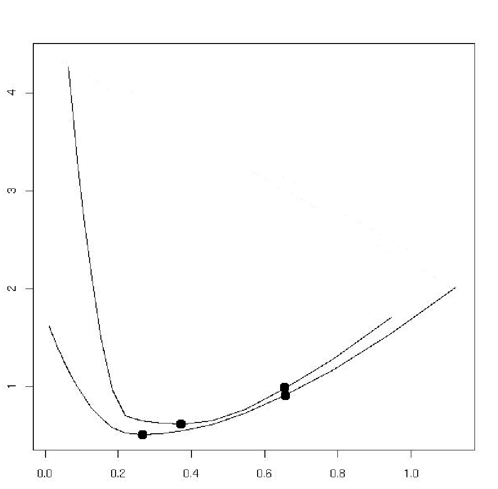
Discussion on the regularization parameter. Finally, we would like to point out the importance of the tuning parameter λ\lambda (in a general term). Figure 2 illustrates a graph of a typical experiment. There are two curves on this graph, that represent the quantities (1/n)​‖X⁡(β^L​(λ)−β∗)‖22(1/n)\|X(\hat{\beta}^{L}(\lambda)-\beta^{*})\|_{2}^{2} and (1/m)​‖Z⁡(β^L​(λ)−β∗)‖22(1/m)\|Z(\hat{\beta}^{L}(\lambda)-\beta^{*})\|_{2}^{2} with respect to λ\lambda. We observe that both functions do not reach their minimum value for the same value of λ\lambda (the minimum is highlighted on the graph by a dot), even if these minimum are quite close.
Refer to caption
Figure 2: Performance vs. λ\lambda.

Since we consider variable selection methods, the identification of the true support {j:βj∗≠0}\{j:\,\beta_{j}^{*}\neq 0\} of the vector β∗\beta^{*} is also in concern. One expects that the estimator β^\hat{\beta} and the true vector β∗\beta^{*} share the same support at least when nn is large enough. This is known as the variable selection consistency problem and it has been considered for the LASSO estimator in several works (see [Bun08, MB06, MY09, Wai06, ZY06]). Recently, [Lou08] provided the variable selection consistency of the Dantzig Selector. Other popular selection procedures, based on the LASSO estimator, such as the Adaptive LASSO [Zou06], the SCAD [FL01], the S-LASSO [Heb08] and the Group-LASSO [Bac08], have also been studied under a variable selection point of view. Following our previous work [AH08], it is possible to provide such results for the Transductive LASSO.

The variable selection task has also been illustrated in Figure 2. We reported the minimal value of λ\lambda for which the LASSO estimator identifies correctly the non zero components of β∗\beta^{*}. This value of λ\lambda is quite different from the values that minimizes the prediction losses. This observation is recurrent in almost all the experiments: the estimation X​β∗X\beta^{*}, Z​β∗Z\beta^{*} and the support of β∗\beta^{*} are three different objectives and have to be treated separately. We cannot expect in general to find a choice for λ\lambda which makes the LASSO, for instance, has good performance for all the mentioned objective simultaneously.

6 Conclusion

In this paper, we propose an extension of the LASSO and the Dantzig Selector for which we provide theoretical results with less restrictive hypothesis than in previous works. These estimators have a nice interpretation in terms of transductive prediction. Moreover, we study the practical performance of the proposed transductive estimators on simulated data. It turns out that the benefit using such methods is emphasized when the model is sparse and particularly when the samples sizes (nn labeled points and mm unlabeled points) and dimension pp are such that n<p<mn<p<m.

7 Proofs

In this section, we state the proofs of our main results.

7.1 Proof of Propositions 3.1 and 3.2

Proof of Proposition 3.1.

Let us assume that (X′​X)(X^{\prime}X) is invertible. Then just remark that the criterion minimized by β^n​I,λ\hat{\beta}_{\sqrt{n}I,\lambda} is just

n​‖β^L​S​E−β‖22+2​λ​‖Ξn​I​β‖1=∑j=1p{[β^jL​S​E−βj]2+2​λ​ξj​(n​I)n​|βj|}.n\left\|\hat{\beta}^{LSE}-\beta\right\|^{2}_{2}+2\lambda\|\Xi_{nI}\beta\|_{1}=\sum_{j=1}^{p}\left\{\left[\hat{\beta}^{LSE}_{j}-\beta_{j}\right]^{2}+\frac{2\lambda\xi_{j}(\sqrt{n}I)}{n}|\beta_{j}|\right\}.

So we can optimize with respect to each coordinate βj\beta_{j} individually. It is quite easy to check that the solution is, for βj\beta_{j},

s​g​n​(β^jL​S​E)​(|β^jL​S​E|−λ​ξj​(n​I)n)+.sgn\left(\hat{\beta}^{LSE}_{j}\right)\left(\left|\hat{\beta}^{LSE}_{j}\right|-\frac{\lambda\xi_{j}(\sqrt{n}I)}{n}\right)_{+}.

The proof for β^n​I,λ\hat{\beta}_{\sqrt{n}I,\lambda} is also easy as it solves

{arg⁡minβ∈ℝp⁡‖β‖1s.t.‖n​Ξn​I−1​(β^L​S​E−β)‖∞≤λ.\left\{\begin{array}[]{l}\arg\min_{\beta\in\mathds{R}^{p}}\left\|\beta\right\|_{1}\\ \\ s.t.\left\|n\Xi_{nI}^{-1}(\hat{\beta}^{LSE}-\beta)\right\|_{\infty}\leq\lambda.\end{array}\right.

∎

Proof of Proposition 3.2.

Let us write the Lagrangian of the program

{arg⁡minβ∈ℝp⁡‖A​β‖22s.t.‖ΞA−1​(A′​A)​((X′​X~)−1​X′​Y−β)‖∞≤λ,\left\{\begin{array}[]{l}\arg\min_{\beta\in\mathds{R}^{p}}\left\|A\beta\right\|_{2}^{2}\\ \\ s.t.\left\|\Xi_{A}^{-1}(A^{\prime}A)((\widetilde{X^{\prime}X})^{-1}X^{\prime}Y-\beta)\right\|_{\infty}\leq\lambda,\end{array}\right.
ℒ⁡(β,γ,μ)=β⁡(Z′​Z)​β+γ′​[ΞA−1​(A′​A)​((X′​X~)−1​X′​Y−β)−λ​E]+μ′​[ΞA−1​(A′​A)​(β−(X′​X~)−1​X′​Y)−λ​E]\mathcal{L}(\beta,\gamma,\mu)=\beta(Z^{\prime}Z)\beta+\gamma^{\prime}\left[\Xi_{A}^{-1}(A^{\prime}A)((\widetilde{X^{\prime}X})^{-1}X^{\prime}Y-\beta)-\lambda E\right]\\ +\mu^{\prime}\left[\Xi_{A}^{-1}(A^{\prime}A)(\beta-(\widetilde{X^{\prime}X})^{-1}X^{\prime}Y)-\lambda E\right]

with E=(1,…,1)′E=(1,\ldots,1)^{\prime}, and for any jj, γj≥0\gamma_{j}\geq 0, μj≥0\mu_{j}\geq 0 and γj​μj=0\gamma_{j}\mu_{j}=0. Any solution β¯=β¯​(γ,μ)\underline{\beta}=\underline{\beta}(\gamma,\mu) must satisfy

0=∂ℒ∂β​(β¯,λ,μ)=2​β¯​(A′​A)+(γ−μ)​ΞA−1​(A′​A)0=\frac{\partial\mathcal{L}}{\partial\beta}(\underline{\beta},\lambda,\mu)=2\underline{\beta}(A^{\prime}A)+(\gamma-\mu)\Xi_{A}^{-1}(A^{\prime}A)

so

(A′​A)​β¯=(A′​A)​ΞA−1​μ−γ2.(A^{\prime}A)\underline{\beta}=(A^{\prime}A)\Xi^{-1}_{A}\frac{\mu-\gamma}{2}.

Note that the conditions γj≥0\gamma_{j}\geq 0, μj≥0\mu_{j}\geq 0 and γj​μj=0\gamma_{j}\mu_{j}=0 means that there is a ζj∈ℝ\zeta_{j}\in\mathds{R} such that ζj=ξj12​(A)​(μj−γj)/2\zeta_{j}=\xi_{j}^{\frac{1}{2}}(A)(\mu_{j}-\gamma_{j})/2, |ζj|=ξj12​(A)​(γj+μj)/2|\zeta_{j}|=\xi_{j}^{\frac{1}{2}}(A)(\gamma_{j}+\mu_{j})/2, and so γj=2​(ζj/ξj12​(A))−\gamma_{j}=2(\zeta_{j}/\xi_{j}^{\frac{1}{2}}(A))_{-} and μj=2​(ζj/ξj12​(A))+\mu_{j}=2(\zeta_{j}/\xi_{j}^{\frac{1}{2}}(A))_{+}, where (a)+=m​a​x​(a,0)(a)_{+}=max(a;0) and (a)−=m​a​x​(−a,0)(a)_{-}=max(-a;0). Let also ζ\zeta denote the vector which jj-th component is exactly ζj\zeta_{j}, we obtain

(A′​A)​β¯=(A′​A)​ζ,(A^{\prime}A)\underline{\beta}=(A^{\prime}A)\zeta,

or, using the condition Ker(A)=Ker(X)\mathop{\rm Ker}\nolimits(A)=\mathop{\rm Ker}\nolimits(X), X​β¯=X​ζX\underline{\beta}=X\zeta and A​β¯=A​ζA\underline{\beta}=A\zeta. This leads to

ℒ⁡(β¯,γ,μ)=−2​Y′​X​(X′​X~)−1​(A′​A)​ζ+ζ′​(A′​A)​ζ+2​λ​‖ΞA​ζ‖1,\mathcal{L}(\underline{\beta},\gamma,\mu)=-2Y^{\prime}X(\widetilde{X^{\prime}X})^{-1}(A^{\prime}A)\zeta+\zeta^{\prime}(A^{\prime}A)\zeta+2\lambda\|\Xi_{A}\zeta\|_{1},

and note that the first order condition also implies that γ\gamma and μ\mu (and so ζ\zeta) maximize ℒ\mathcal{L}. This ends the proof. ∎

7.2 A useful Lemma

The following lemma will be used in the proofs of Theorems 3.3 and 3.4.

Lemma 7.1.

Let us put ε=(ε1,…,εn)′\varepsilon=(\varepsilon_{1},\ldots,\varepsilon_{n})^{\prime}. If Ker(A)=Ker(X)\mathop{\rm Ker}\nolimits(A)=\mathop{\rm Ker}\nolimits(X) we have, with probability at least 1−η1-\eta,

∀j∈{1,…,p},|[A′​A​(X′​X~)−1​X′​ε]j|≤ξj​(A)​σ​2​n​log⁡pη,\forall j\in\{1,\ldots,p\},\left|\left[A^{\prime}A(\widetilde{X^{\prime}X})^{-1}X^{\prime}\varepsilon\right]_{j}\right|\leq\xi_{j}(A)\sigma\sqrt{2n\log\frac{p}{\eta}},

or, in other words,

‖ΞA−1​(A′​A)​((X′​X~)−1​X′​Y−β∗)‖∞≤σ​2​n​log⁡pη.\|\Xi^{-1}_{A}(A^{\prime}A)((\widetilde{X^{\prime}X})^{-1}X^{\prime}Y-\beta^{*})\|_{\infty}\leq\sigma\sqrt{2n\log\frac{p}{\eta}}.
Proof of the lemma.

By definition, ε∼𝒩⁡(0,σ2​I)\varepsilon\sim\mathcal{N}(0,\sigma^{2}I) and so

(A′​A)​(X′​X~)−1​X′​ε∼𝒩⁡(0,σ2​(A′​A)​(X′​X~)−1​(A′​A)).(A^{\prime}A)(\widetilde{X^{\prime}X})^{-1}X^{\prime}\varepsilon\sim\mathcal{N}(0,\sigma^{2}(A^{\prime}A)(\widetilde{X^{\prime}X})^{-1}(A^{\prime}A)).

So, for all jj, [(A′​A)​(X′​X~)−1​X′​ε]j[(A^{\prime}A)(\widetilde{X^{\prime}X})^{-1}X^{\prime}\varepsilon]_{j} comes from a 𝒩⁡(0,σ2​ξj2​(A))\mathcal{N}(0,\sigma^{2}\xi_{j}^{2}(A)) distribution. This implies the first point, the second one is trivial using Y=X​β∗+εY=X\beta^{*}+\varepsilon. ∎

7.3 Proof of Theorems 3.3 and 3.4

Proof of Theorem 3.3.

By definition of β^A,λ\hat{\beta}_{A,\lambda} we have

−2​Y′​X​(X′​X~)−1​(A′​A)​β^A,λ+(β^A,λ)′​(A′​A)​β^A,λ+2​λ​‖ΞA′​A​β^A,λ‖1≤2​Y′​X​(X′​X~)−1​(A′​A)​β∗+(β∗)′​(A′​A)​β∗+2​λ​‖ΞA​β∗‖1.-2Y^{\prime}X(\widetilde{X^{\prime}X})^{-1}(A^{\prime}A)\hat{\beta}_{A,\lambda}+\left(\hat{\beta}_{A,\lambda}\right)^{\prime}(A^{\prime}A)\hat{\beta}_{A,\lambda}+2\lambda\|\Xi_{A^{\prime}A}\hat{\beta}_{A,\lambda}\|_{1}\\ \leq 2Y^{\prime}X(\widetilde{X^{\prime}X})^{-1}(A^{\prime}A)\beta^{*}+(\beta^{*})^{\prime}(A^{\prime}A)\beta^{*}+2\lambda\|\Xi_{A}\beta^{*}\|_{1}.

Since Y=X​β∗+εY=X\beta^{*}+\varepsilon, we obtain

2​(β∗)′​X′​X​(X′​X~)−1​(A′​A)​(β∗−β^A,λ)+(β^A,λ)′​(A′​A)​β^A,λ−(β∗)′​(A′​A)​β∗+2​ε′​X​(X′​X~)−1​(A′​A)​(β∗−β^A,λ)≤2​λ​‖ΞA​β∗‖1−2​λ​‖ΞA​β^A,λ‖1.2(\beta^{*})^{\prime}X^{\prime}X(\widetilde{X^{\prime}X})^{-1}(A^{\prime}A)\left(\beta^{*}-\hat{\beta}_{A,\lambda}\right)+\left(\hat{\beta}_{A,\lambda}\right)^{\prime}(A^{\prime}A)\hat{\beta}_{A,\lambda}-(\beta^{*})^{\prime}(A^{\prime}A)\beta^{*}\\ +2\varepsilon^{\prime}X(\widetilde{X^{\prime}X})^{-1}(A^{\prime}A)\left(\beta^{*}-\hat{\beta}_{A,\lambda}\right)\leq 2\lambda\|\Xi_{A}\beta^{*}\|_{1}-2\lambda\|\Xi_{A}\hat{\beta}_{A,\lambda}\|_{1}.

Now, if Ker(X)=Ker(A)\mathop{\rm Ker}\nolimits(X)=\mathop{\rm Ker}\nolimits(A) then we have X′​X​(X′​X~)−1​(A′​A)=(A′​A)X^{\prime}X(\widetilde{X^{\prime}X})^{-1}(A^{\prime}A)=(A^{\prime}A) and then the previous inequality leads to

(β∗−β^A,λ)′​(A′​A)​(β∗−β^A,λ)≤2​ε′​X​(X′​X~)−1​(A′​A)​(β^A,λ−β∗)+2​λ​‖ΞA​β∗‖1−2​λ​‖ΞA​β^A,λ‖1.\left(\beta^{*}-\hat{\beta}_{A,\lambda}\right)^{\prime}(A^{\prime}A)\left(\beta^{*}-\hat{\beta}_{A,\lambda}\right)\\ \leq 2\varepsilon^{\prime}X(\widetilde{X^{\prime}X})^{-1}(A^{\prime}A)\left(\hat{\beta}_{A,\lambda}-\beta^{*}\right)+2\lambda\|\Xi_{A}\beta^{*}\|_{1}-2\lambda\|\Xi_{A}\hat{\beta}_{A,\lambda}\|_{1}. (9)

Now we have to work on the term 2​ε′​X​(X′​X~)−1​(A′​A)​(β^A,λ−β∗)2\varepsilon^{\prime}X(\widetilde{X^{\prime}X})^{-1}(A^{\prime}A)\left(\hat{\beta}_{A,\lambda}-\beta^{*}\right). Note that

2​ε′​X​(X′​X~)−1​(A′​A)​(β^A,λ−β∗)\displaystyle 2\varepsilon^{\prime}X(\widetilde{X^{\prime}X})^{-1}(A^{\prime}A)\left(\hat{\beta}_{A,\lambda}-\beta^{*}\right) =\displaystyle= 2​∑j=1p(β^A,λ−β∗)j​[(A′​A)​(X′​X~)−1​X′​ε]j\displaystyle 2\sum_{j=1}^{p}\left(\hat{\beta}_{A,\lambda}-\beta^{*}\right)_{j}\left[(A^{\prime}A)(\widetilde{X^{\prime}X})^{-1}X^{\prime}\varepsilon\right]_{j}
≤\displaystyle\leq 2​∑j=1p|(β^A,λ−β∗)j|​|[(A′​A)​(X′​X~)−1​X′​ε]j|\displaystyle 2\sum_{j=1}^{p}\left|\left(\hat{\beta}_{A,\lambda}-\beta^{*}\right)_{j}\right|\left|\left[(A^{\prime}A)(\widetilde{X^{\prime}X})^{-1}X^{\prime}\varepsilon\right]_{j}\right|
≤\displaystyle\leq 2​σ​2​n​log⁡(pη)​∑j=1pξj12​(A)​|(β^A,λ)j−βj∗|\displaystyle 2\sigma\sqrt{2n\log\left(\frac{p}{\eta}\right)}\sum_{j=1}^{p}\xi_{j}^{\frac{1}{2}}(A)\left|\left(\hat{\beta}_{A,\lambda}\right)_{j}-\beta^{*}_{j}\right|

with probability at least 1−η1-\eta, by Lemma 7.1. We plug this result into Inequality (9) (and replace λ\lambda by its value 2​σ​2​n​log⁡(p/η)2\sigma\sqrt{2n\log(p/\eta)}) to obtain

(β∗−β^A,λ)′​(A′​A)​(β∗−β^A,λ)≤2​σ​2​n​log⁡(pη)​∑j=1pξj12​(A)​{|(β^A,λ)j−βj∗|+2​(|βj∗|−|(β^A,λ)j|)}\left(\beta^{*}-\hat{\beta}_{A,\lambda}\right)^{\prime}(A^{\prime}A)\left(\beta^{*}-\hat{\beta}_{A,\lambda}\right)\\ \leq 2\sigma\sqrt{2n\log\left(\frac{p}{\eta}\right)}\sum_{j=1}^{p}\xi_{j}^{\frac{1}{2}}(A)\Biggl\{\left|\left(\hat{\beta}_{A,\lambda}\right)_{j}-\beta^{*}_{j}\right|+2\left(\left|\beta^{*}_{j}\right|-\left|\left(\hat{\beta}_{A,\lambda}\right)_{j}\right|\right)\Biggr\}

and then

(β∗−β^A,λ)′​(A′​A)​(β∗−β^A,λ)\displaystyle\left(\beta^{*}-\hat{\beta}_{A,\lambda}\right)^{\prime}(A^{\prime}A)\left(\beta^{*}-\hat{\beta}_{A,\lambda}\right) (10)
+2σ2​n​log⁡(pη)∑j=1pξj12(A)|(β^A,λ)j−βj∗|\displaystyle+2\sigma\sqrt{2n\log\left(\frac{p}{\eta}\right)}\sum_{j=1}^{p}\xi_{j}^{\frac{1}{2}}(A)\left|\left(\hat{\beta}_{A,\lambda}\right)_{j}-\beta^{*}_{j}\right|
≤\displaystyle\leq 4​σ​2​n​log⁡(pη)​∑j=1pξj12​(A)​{|(β^A,λ)j−βj∗|+|βj∗|−|(β^A,λ)j|}\displaystyle 4\sigma\sqrt{2n\log\left(\frac{p}{\eta}\right)}\sum_{j=1}^{p}\xi_{j}^{\frac{1}{2}}(A)\Biggl\{\left|\left(\hat{\beta}_{A,\lambda}\right)_{j}-\beta^{*}_{j}\right|+\left|\beta^{*}_{j}\right|-\left|\left(\hat{\beta}_{A,\lambda}\right)_{j}\right|\Biggr\}
=\displaystyle= 4σ2​n​log⁡(pη)∑j:βj∗≠0ξj12(A){|(β^A,λ)j−βj∗|+|βj∗|−|(β^A,λ)j|}\displaystyle 4\sigma\sqrt{2n\log\left(\frac{p}{\eta}\right)}\sum_{j:\beta^{*}_{j}\neq 0}\xi_{j}^{\frac{1}{2}}(A)\Biggl\{\left|\left(\hat{\beta}_{A,\lambda}\right)_{j}-\beta^{*}_{j}\right|+\left|\beta^{*}_{j}\right|-\left|\left(\hat{\beta}_{A,\lambda}\right)_{j}\right|\Biggr\}
≤\displaystyle\leq 8σ2​n​log⁡(pη)∑j:βj∗≠0ξj12(A)|(β^A,λ)j−βj∗|.\displaystyle 8\sigma\sqrt{2n\log\left(\frac{p}{\eta}\right)}\sum_{j:\beta^{*}_{j}\neq 0}\xi_{j}^{\frac{1}{2}}(A)\left|\left(\hat{\beta}_{A,\lambda}\right)_{j}-\beta^{*}_{j}\right|.

This implies, in particular, that β∗−β^A,λ\beta^{*}-\hat{\beta}_{A,\lambda} is an admissible vector α\alpha in Assumption H⁡(A′​A,3)H(A^{\prime}A,3) because

∑j=1pξj12(A)|(β^A,λ)j−βj∗|≤4∑j:βj∗≠0ξj12(A)|(β^A,λ)j−βj∗|.\sum_{j=1}^{p}\xi_{j}^{\frac{1}{2}}(A)\left|\left(\hat{\beta}_{A,\lambda}\right)_{j}-\beta^{*}_{j}\right|\leq 4\sum_{j:\beta^{*}_{j}\neq 0}\xi_{j}^{\frac{1}{2}}(A)\left|\left(\hat{\beta}_{A,\lambda}\right)_{j}-\beta^{*}_{j}\right|.

On the other hand, thanks to Inequality (10), we have

(β∗−β^A,λ)′​(A′​A)​(β∗−β^A,λ)≤6σ2​n​log⁡(pη)∑j:βj∗≠0ξj12(A)|(β^A,λ)j−β∗j|≤6σ2n∑j:βj∗≠0[(β^A,λ)j−β∗j]2∑j:βj∗≠0ξj(A)log(pη)≤6σ2c⁡(A′​A)(β∗−β^A,λ)′(A′A)(β∗−β^A,λ)∑j:βj∗≠0ξj(M)log(pη),\left(\beta^{*}-\hat{\beta}_{A,\lambda}\right)^{\prime}(A^{\prime}A)\left(\beta^{*}-\hat{\beta}_{A,\lambda}\right)\\ \leq 6\sigma\sqrt{2n\log\left(\frac{p}{\eta}\right)}\sum_{j:\beta^{*}_{j}\neq 0}\xi_{j}^{\frac{1}{2}}(A)\left|\left(\hat{\beta}_{A,\lambda}\right)_{j}-\beta^{*}_{j}\right|\\ \leq 6\sigma\sqrt{2n\sum_{j:\beta^{*}_{j}\neq 0}\left[\left(\hat{\beta}_{A,\lambda}\right)_{j}-\beta^{*}_{j}\right]^{2}\sum_{j:\beta^{*}_{j}\neq 0}\xi_{j}(A)\log\left(\frac{p}{\eta}\right)}\\ \leq 6\sigma\sqrt{\frac{2}{c(A^{\prime}A)}\left(\beta^{*}-\hat{\beta}_{A,\lambda}\right)^{\prime}(A^{\prime}A)\left(\beta^{*}-\hat{\beta}_{A,\lambda}\right)\sum_{j:\beta^{*}_{j}\neq 0}\xi_{j}(M)\log\left(\frac{p}{\eta}\right)}, (11)

where we used Assumption H⁡(A′​A,3)H(A^{\prime}A,3) for the last inequality. Then

(β∗−β^A,λ)′(A′A)(β∗−β^A,λ)≤72σ2c⁡(A′​A)log(pη)∑j:βj∗≠0ξj(A).\left(\beta^{*}-\hat{\beta}_{A,\lambda}\right)^{\prime}(A^{\prime}A)\left(\beta^{*}-\hat{\beta}_{A,\lambda}\right)\leq 72\frac{\sigma^{2}}{c(A^{\prime}A)}\log\left(\frac{p}{\eta}\right)\sum_{j:\beta^{*}_{j}\neq 0}\xi_{j}(A). (12)

A similar reasoning as in (11) leads to

2​σ​2​n​log⁡(pη)​∑j=1pξj12​(A)​|(β^A,λ)j−βj∗|≤8σ2c⁡(A′​A)(β∗−β^A,λ)′(A′A)(β∗−β^A,λ)∑j:βj∗≠0ξj(M)log(pη).2\sigma\sqrt{2n\log\left(\frac{p}{\eta}\right)}\sum_{j=1}^{p}\xi_{j}^{\frac{1}{2}}(A)\left|\left(\hat{\beta}_{A,\lambda}\right)_{j}-\beta^{*}_{j}\right|\\ \leq 8\sigma\sqrt{\frac{2}{c(A^{\prime}A)}\left(\beta^{*}-\hat{\beta}_{A,\lambda}\right)^{\prime}(A^{\prime}A)\left(\beta^{*}-\hat{\beta}_{A,\lambda}\right)\sum_{j:\beta^{*}_{j}\neq 0}\xi_{j}(M)\log\left(\frac{p}{\eta}\right)}.

Finally, combine this last inequality with (12) to obtain the desired bound for ‖ΞA​(β∗−β^A,λ)‖1.\left\|\Xi_{A}\left(\beta^{*}-\hat{\beta}_{A,\lambda}\right)\right\|_{1}. This ends the proof. ∎

Proof of Theorem 3.4.

We have

(β~A,λ−β∗)′​(A′​A)​(β~A,λ−β∗)=[ΞA​(β~A,λ−β∗)]′​ΞA−1​(A′​A)​(β~A,λ−β∗)≤‖ΞA​(β~A,λ−β∗)‖1​‖ΞA−1​(A′​A)​(β~A,λ−β∗)‖∞≤∥ΞA(β~A,λ−β∗)∥1{∥Ξ−1A(A′A)((X′​X~)−1X′Y−β∗)∥∞+∥Ξ−1A(A′A)((X′​X~)−1X′Y−β~A,λ)∥∞},(\tilde{\beta}_{A,\lambda}-\beta^{*})^{\prime}(A^{\prime}A)(\tilde{\beta}_{A,\lambda}-\beta^{*})=[\Xi_{A}(\tilde{\beta}_{A,\lambda}-\beta^{*})]^{\prime}\Xi^{-1}_{A}(A^{\prime}A)(\tilde{\beta}_{A,\lambda}-\beta^{*})\\ \leq\|\Xi_{A}(\tilde{\beta}_{A,\lambda}-\beta^{*})\|_{1}\|\Xi^{-1}_{A}(A^{\prime}A)(\tilde{\beta}_{A,\lambda}-\beta^{*})\|_{\infty}\\ \leq\|\Xi_{A}(\tilde{\beta}_{A,\lambda}-\beta^{*})\|_{1}\Biggl\{\|\Xi^{-1}_{A}(A^{\prime}A)((\widetilde{X^{\prime}X})^{-1}X^{\prime}Y-\beta^{*})\|_{\infty}\\ +\|\Xi^{-1}_{A}(A^{\prime}A)((\widetilde{X^{\prime}X})^{-1}X^{\prime}Y-\tilde{\beta}_{A,\lambda})\|_{\infty}\Biggr\}, (13)

by the constraint in the definition on β~A,λ\tilde{\beta}_{A,\lambda} we have

‖ΞA−1​(A′​A)​((X′​X~)−1​X′​Y−β~A,λ)‖∞≤λ,\|\Xi^{-1}_{A}(A^{\prime}A)((\widetilde{X^{\prime}X})^{-1}X^{\prime}Y-\tilde{\beta}_{A,\lambda})\|_{\infty}\leq\lambda,

while Lemma 7.1 implies that for λ=2​σ​2​n​log⁡(p/η)\lambda=2\sigma\sqrt{2n\log(p/\eta)} we have

‖ΞA−1​(A′​A)​((X′​X~)−1​X′​Y−β∗)‖∞≤λ2,\|\Xi^{-1}_{A}(A^{\prime}A)((\widetilde{X^{\prime}X})^{-1}X^{\prime}Y-\beta^{*})\|_{\infty}\leq\frac{\lambda}{2},

with probability at least 1−η1-\eta; and so:

(β~A,λ−β∗)′​(A′​A)​(β~A,λ−β∗)≤3​λ2​‖ΞA​(β~A,λ−β∗)‖1.(\tilde{\beta}_{A,\lambda}-\beta^{*})^{\prime}(A^{\prime}A)(\tilde{\beta}_{A,\lambda}-\beta^{*})\leq\frac{3\lambda}{2}\|\Xi_{A}(\tilde{\beta}_{A,\lambda}-\beta^{*})\|_{1}.

Moreover note that, by definition,

0≤‖ΞA​β∗‖1−‖ΞA​β~A,λ‖1=∑βj∗≠0ξj12​(A)​|βj∗|−∑βj∗≠0ξj12​(A)​|(β~A,λ)j|−∑βj∗=0ξj12​(A)​|(β~A,λ)j|≤∑βj∗≠0ξj12​(A)​|βj∗−(β~A,λ)j|−∑βj∗=0ξj12​(A)​|βj∗−(β~A,λ)j|,0\leq\|\Xi_{A}\beta^{*}\|_{1}-\|\Xi_{A}\tilde{\beta}_{A,\lambda}\|_{1}\\ =\sum_{\beta^{*}_{j}\neq 0}\xi_{j}^{\frac{1}{2}}(A)\left|\beta^{*}_{j}\right|-\sum_{\beta^{*}_{j}\neq 0}\xi_{j}^{\frac{1}{2}}(A)\left|(\tilde{\beta}_{A,\lambda})_{j}\right|-\sum_{\beta^{*}_{j}=0}\xi_{j}^{\frac{1}{2}}(A)\left|(\tilde{\beta}_{A,\lambda})_{j}\right|\\ \leq\sum_{\beta^{*}_{j}\neq 0}\xi_{j}^{\frac{1}{2}}(A)\left|\beta^{*}_{j}-(\tilde{\beta}_{A,\lambda})_{j}\right|-\sum_{\beta^{*}_{j}=0}\xi_{j}^{\frac{1}{2}}(A)\left|\beta^{*}_{j}-(\tilde{\beta}_{A,\lambda})_{j}\right|,

this implies that β∗−(β~A,λ)\beta^{*}-(\tilde{\beta}_{A,\lambda}) is an admissible vector in the relation that defines Assumption H⁡(A′​A,1)H(A^{\prime}A,1). Let us combine this result with Inequality (13), we obtain

(β~A,λ−β∗)′​(A′​A)​(β~A,λ−β∗)≤3​λ2​‖ΞA​(β∗−β~A,λ)‖1≤3​λ​∑βj∗≠0ξj12​(A)​|βj∗−(β~A,λ)j|≤3​λ​(∑βj∗≠0ξj​(A))​(∑βj∗≠0|βj∗−(β~A,λ)j|2)≤3​λ​(∑βj∗≠0ξj​(A))12​1n​c​(A′​A)​(β~A,λ−β∗)′​(A′​A)​(β~A,λ−β∗).(\tilde{\beta}_{A,\lambda}-\beta^{*})^{\prime}(A^{\prime}A)(\tilde{\beta}_{A,\lambda}-\beta^{*})\leq\frac{3\lambda}{2}\|\Xi_{A}(\beta^{*}-\tilde{\beta}_{A,\lambda})\|_{1}\\ \leq 3\lambda\sum_{\beta^{*}_{j}\neq 0}\xi_{j}^{\frac{1}{2}}(A)\left|\beta^{*}_{j}-(\tilde{\beta}_{A,\lambda})_{j}\right|\\ \leq 3\lambda\sqrt{\left(\sum_{\beta^{*}_{j}\neq 0}\xi_{j}(A)\right)\left(\sum_{\beta^{*}_{j}\neq 0}\left|\beta^{*}_{j}-(\tilde{\beta}_{A,\lambda})_{j}\right|^{2}\right)}\\ \leq 3\lambda\left(\sum_{\beta^{*}_{j}\neq 0}\xi_{j}(A)\right)^{\frac{1}{2}}\sqrt{\frac{1}{nc(A^{\prime}A)}(\tilde{\beta}_{A,\lambda}-\beta^{*})^{\prime}(A^{\prime}A)(\tilde{\beta}_{A,\lambda}-\beta^{*})}. (14)

So we have,

(β~A,λ−β∗)′​(A′​A)​(β~A,λ−β∗)≤9​λ2​1n​c​(A′​A)​∑βj∗≠0ξj​(A),(\tilde{\beta}_{A,\lambda}-\beta^{*})^{\prime}(A^{\prime}A)(\tilde{\beta}_{A,\lambda}-\beta^{*})\leq 9\lambda^{2}\frac{1}{nc(A^{\prime}A)}\sum_{\beta^{*}_{j}\neq 0}\xi_{j}(A),

and as a consequence, Inequality (14) gives the upper bound on ‖ΞA​(β~A,λ−β∗)‖1\|\Xi_{A}(\tilde{\beta}_{A,\lambda}-\beta^{*})\|_{1}, and this ends the proof. ∎

7.4 Proof of Theorem 4.1

Proof of Theorem 4.1.

The proof is almost the same as in the previous case. For the sake of simplicity, let us write β~∗\tilde{\beta}^{*} instead of β~n/m​Z,λ2∗\tilde{\beta}^{*}_{\sqrt{n/m}Z,\lambda_{2}} and the same for β^∗\hat{\beta}^{*}. We first give a look at the Dantzig Selector:

nm​(β~∗−β∗)′​Z′​Z​(β~∗−β∗)≤‖β~∗−β∗‖1​‖nm​Z′​Z​(β~∗−β∗)‖∞≤‖β~∗−β∗‖1​{‖nm​Z′​(Z​β~∗−Yˇλ1)‖∞+‖nm​Z′​(Z​β∗−Yˇλ1)‖∞}≤‖β~∗−β∗‖1{‖nmZ′(Zβ~∗−Yˇλ1)‖∞+‖X′(Xβ∗−Y)‖∞+‖X′(Xβ~X,λ1−Y)‖∞+‖(nmZ′Z−X′X)(β∗−β~X,λ1)‖∞}.\frac{n}{m}\left(\tilde{\beta}^{*}-\beta^{*}\right)^{\prime}Z^{\prime}Z\left(\tilde{\beta}^{*}-\beta^{*}\right)\leq\left\|\tilde{\beta}^{*}-\beta^{*}\right\|_{1}\left\|\frac{n}{m}Z^{\prime}Z\left(\tilde{\beta}^{*}-\beta^{*}\right)\right\|_{\infty}\\ \leq\left\|\tilde{\beta}^{*}-\beta^{*}\right\|_{1}\Biggl\{\left\|\frac{n}{m}Z^{\prime}\left(Z\tilde{\beta}^{*}-\check{Y}_{\lambda_{1}}\right)\right\|_{\infty}+\left\|\frac{n}{m}Z^{\prime}\left(Z\beta^{*}-\check{Y}_{\lambda_{1}}\right)\right\|_{\infty}\Biggr\}\\ \leq\left\|\tilde{\beta}^{*}-\beta^{*}\right\|_{1}\Biggl\{\left\|\frac{n}{m}Z^{\prime}\left(Z\tilde{\beta}^{*}-\check{Y}_{\lambda_{1}}\right)\right\|_{\infty}+\left\|X^{\prime}\left(X\beta^{*}-Y\right)\right\|_{\infty}\\ +\left\|X^{\prime}\left(X\tilde{\beta}_{X,\lambda_{1}}-Y\right)\right\|_{\infty}+\left\|\left(\frac{n}{m}Z^{\prime}Z-X^{\prime}X\right)\left(\beta^{*}-\tilde{\beta}_{X,\lambda_{1}}\right)\right\|_{\infty}\Biggr\}. (15)

By Lemma 7.1, for λ1=10−1​σ​2​n​log⁡(p/η)\lambda_{1}=10^{-1}\sigma\sqrt{2n\log(p/\eta)} we have

‖X′​Y−X′​X​β∗‖∞≤10​λ1,\|X^{\prime}Y-X^{\prime}X\beta^{*}\|_{\infty}\leq 10\lambda_{1},

with probability at least 1−η1-\eta. On the other hand, we have

‖β∗−β~X,λ1‖1≤‖β∗‖1+‖β~X,λ1‖1≤2​‖β∗‖1,\|\beta^{*}-\tilde{\beta}_{X,\lambda_{1}}\|_{1}\leq\|\beta^{*}\|_{1}+\|\tilde{\beta}_{X,\lambda_{1}}\|_{1}\leq 2\|\beta^{*}\|_{1},

by definition of the Dantzig Selector. Then, let u=(β∗−β~X,λ1)/2u=(\beta^{*}-\tilde{\beta}_{X,\lambda_{1}})/2 and use Inequality (8) for this specific uu. This ensures that

‖(nm​Z′​Z−X′​X)​(β∗−β~X,λ1)‖∞≤2​λ1.\left\|\left(\frac{n}{m}Z^{\prime}Z-X^{\prime}X\right)\left(\beta^{*}-\tilde{\beta}_{X,\lambda_{1}}\right)\right\|_{\infty}\leq 2\lambda_{1}. (16)

The definition of the Dantzig Selector also implies that

‖X′​(X​β~X,λ1−Y)‖∞≤λ1,\left\|X^{\prime}\left(X\tilde{\beta}_{X,\lambda_{1}}-Y\right)\right\|_{\infty}\leq\lambda_{1},

and finally the definition of the estimator leads to

‖nm​Z′​(Z​β~∗−Yˇλ1)‖∞≤λ2=λ1,\left\|\frac{n}{m}Z^{\prime}\left(Z\tilde{\beta}^{*}-\check{Y}_{\lambda_{1}}\right)\right\|_{\infty}\leq\lambda_{2}=\lambda_{1},

and as a consequence, Inequality (15) becomes

nm​(β~∗−β∗)′​Z′​Z​(β~∗−β∗)≤14​λ1​‖β~∗−β∗‖1.\frac{n}{m}\left(\tilde{\beta}^{*}-\beta^{*}\right)^{\prime}Z^{\prime}Z\left(\tilde{\beta}^{*}-\beta^{*}\right)\leq 14\lambda_{1}\left\|\tilde{\beta}^{*}-\beta^{*}\right\|_{1}.

Using the fact that ‖β~∗‖1≤‖β∗‖1\|\tilde{\beta}^{*}\|_{1}\leq\|\beta^{*}\|_{1} gives

nm​(β~∗−β∗)′​Z′​Z​(β~∗−β∗)≤14​λ1​‖β~∗−β∗‖1≤28​λ1​∑βj∗≠0|βj∗−(β~∗)j|≤28λ1|{j:βj∗≠0}|​(∑βj∗≠0|βj∗−(β~∗)j|2)≤28​λ1​|{j:βj∗≠0}|12​1n​c​(n/m⁡(Z′​Z))​nm​(β~∗−β∗)′​Z′​Z​(β~∗−β∗).\frac{n}{m}\left(\tilde{\beta}^{*}-\beta^{*}\right)^{\prime}Z^{\prime}Z\left(\tilde{\beta}^{*}-\beta^{*}\right)\leq 14\lambda_{1}\left\|\tilde{\beta}^{*}-\beta^{*}\right\|_{1}\leq 28\lambda_{1}\sum_{\beta^{*}_{j}\neq 0}\left|\beta^{*}_{j}-(\tilde{\beta}^{*})_{j}\right|\\ \leq 28\lambda_{1}\sqrt{\left|\left\{j:\beta^{*}_{j}\neq 0\right\}\right|\left(\sum_{\beta^{*}_{j}\neq 0}\left|\beta^{*}_{j}-(\tilde{\beta}^{*})_{j}\right|^{2}\right)}\\ \leq 28\lambda_{1}\left|\left\{j:\beta^{*}_{j}\neq 0\right\}\right|^{\frac{1}{2}}\sqrt{\frac{1}{nc(n/m(Z^{\prime}Z))}\frac{n}{m}\left(\tilde{\beta}^{*}-\beta^{*}\right)^{\prime}Z^{\prime}Z\left(\tilde{\beta}^{*}-\beta^{*}\right)}. (17)

To establish the last inequality, we used Assumption H′​((n/m)​Z′​Z,1)H^{\prime}((n/m)Z^{\prime}Z,1). Then we have,

nm​(β~∗−β∗)′​Z′​Z​(β~∗−β∗)≤282​λ12​|{j:βj∗≠0}|​1n​c​(n/m⁡(Z′​Z)),\frac{n}{m}\left(\tilde{\beta}^{*}-\beta^{*}\right)^{\prime}Z^{\prime}Z\left(\tilde{\beta}^{*}-\beta^{*}\right)\leq 28^{2}\lambda_{1}^{2}\left|\left\{j:\beta^{*}_{j}\neq 0\right\}\right|\frac{1}{nc(n/m(Z^{\prime}Z))},

This inequality, combined with (17), end the proof for the Dantzig Selector.

Now, let us deal with the LASSO case. The dual form of the definition of the estimator leads to

−2​nm​Yˇλ1​Z​β^∗+nm​(β^∗)′​Z′​Z​β^∗+40​λ2​‖β^∗‖1≤−2​nm​Yˇλ1​Z​β∗+nm​(β∗)′​Z′​Z​β∗+40​λ2​‖β∗‖1-2\frac{n}{m}\check{Y}_{\lambda_{1}}Z\hat{\beta}^{*}+\frac{n}{m}(\hat{\beta}^{*})^{\prime}Z^{\prime}Z\hat{\beta}^{*}+40\lambda_{2}\|\hat{\beta}^{*}\|_{1}\\ \leq-2\frac{n}{m}\check{Y}_{\lambda_{1}}Z\beta^{*}+\frac{n}{m}(\beta^{*})^{\prime}Z^{\prime}Z\beta^{*}+40\lambda_{2}\|\beta^{*}\|_{1}

and so

−2​nm​β~X,λ1​Z′​Z​β^∗+nm​(β^∗)′​Z′​Z​β^∗+40​λ2​‖β^∗‖1≤−2​nm​β~X,λ1​Z′​Z​β∗+nm​(β∗)′​Z′​Z​β∗+40​λ2​‖β∗‖1.-2\frac{n}{m}\tilde{\beta}_{X,\lambda_{1}}Z^{\prime}Z\hat{\beta}^{*}+\frac{n}{m}(\hat{\beta}^{*})^{\prime}Z^{\prime}Z\hat{\beta}^{*}+40\lambda_{2}\|\hat{\beta}^{*}\|_{1}\\ \leq-2\frac{n}{m}\tilde{\beta}_{X,\lambda_{1}}Z^{\prime}Z\beta^{*}+\frac{n}{m}(\beta^{*})^{\prime}Z^{\prime}Z\beta^{*}+40\lambda_{2}\|\beta^{*}\|_{1}.

As a consequence,

nm​(β^∗−β∗)′​Z′​Z​(β^∗−β∗)≤2​nm​(β^∗−β∗)′​Z′​Z​(β~X,λ1−β∗)+40​λ2​(‖β∗‖1−‖β^∗‖1).\frac{n}{m}\left(\hat{\beta}^{*}-\beta^{*}\right)^{\prime}Z^{\prime}Z\left(\hat{\beta}^{*}-\beta^{*}\right)\\ \leq 2\frac{n}{m}\left(\hat{\beta}^{*}-\beta^{*}\right)^{\prime}Z^{\prime}Z\left(\tilde{\beta}_{X,\lambda_{1}}-\beta^{*}\right)+40\lambda_{2}\left(\|\beta^{*}\|_{1}-\|\hat{\beta}^{*}\|_{1}\right).

Now, we try to upper bound (β^∗−β∗)′​Z′​Z​(β~X,λ1−β∗)\left(\hat{\beta}^{*}-\beta^{*}\right)^{\prime}Z^{\prime}Z\left(\tilde{\beta}_{X,\lambda_{1}}-\beta^{*}\right). We remark that

nm​(β^∗−β∗)′​Z′​Z​(β~X,λ1−β∗)≤‖β^∗−β∗‖1​‖nm​(Z′​Z)​(β~X,λ1−β∗)‖∞\displaystyle\frac{n}{m}\left(\hat{\beta}^{*}-\beta^{*}\right)^{\prime}Z^{\prime}Z\left(\tilde{\beta}_{X,\lambda_{1}}-\beta^{*}\right)\leq\left\|\hat{\beta}^{*}-\beta^{*}\right\|_{1}\left\|\frac{n}{m}(Z^{\prime}Z)\left(\tilde{\beta}_{X,\lambda_{1}}-\beta^{*}\right)\right\|_{\infty}
≤\displaystyle\leq ‖β^∗−β∗‖1[‖((nmZ′Z−X′X)(β~X,λ1−β∗)‖∞\displaystyle\left\|\hat{\beta}^{*}-\beta^{*}\right\|_{1}\Biggl[\left\|\left((\frac{n}{m}Z^{\prime}Z-X^{\prime}X\right)\left(\tilde{\beta}_{X,\lambda_{1}}-\beta^{*}\right)\right\|_{\infty}
+‖X′X(β~X,λ1−β∗)‖∞]≤13λ1‖β^∗−β∗‖1,\displaystyle+\left\|X^{\prime}X\left(\tilde{\beta}_{X,\lambda_{1}}-\beta^{*}\right)\right\|_{\infty}\Biggr]\leq 13\lambda_{1}\left\|\hat{\beta}^{*}-\beta^{*}\right\|_{1},

where we used (16) and the fact that

‖X′​X​(β~X,λ1−β∗)‖∞≤‖X′​(X​β~X,λ1−Y)‖∞+‖X′​ε‖∞≤λ1+10​λ1=11​λ1.\left\|X^{\prime}X\left(\tilde{\beta}_{X,\lambda_{1}}-\beta^{*}\right)\right\|_{\infty}\leq\left\|X^{\prime}\left(X\tilde{\beta}_{X,\lambda_{1}}-Y\right)\right\|_{\infty}+\left\|X^{\prime}\varepsilon\right\|_{\infty}\leq\lambda_{1}+10\lambda_{1}=11\lambda_{1}.

Then we have

nm​(β^∗−β∗)′​Z′​Z​(β^∗−β∗)≤26​λ1​‖β^∗−β∗‖1+40​λ2​(‖β∗‖1−‖β^∗‖1),\frac{n}{m}\left(\hat{\beta}^{*}-\beta^{*}\right)^{\prime}Z^{\prime}Z\left(\hat{\beta}^{*}-\beta^{*}\right)\\ \leq 26\lambda_{1}\left\|\hat{\beta}^{*}-\beta^{*}\right\|_{1}+40\lambda_{2}\left(\|\beta^{*}\|_{1}-\|\hat{\beta}^{*}\|_{1}\right),

and so

nm​(β^∗−β∗)′​Z′​Z​(β^∗−β∗)+14​λ1​‖β^∗−β∗‖1≤40​λ1​(‖β^∗−β∗‖1+‖β∗‖1−‖β^∗‖1).\frac{n}{m}\left(\hat{\beta}^{*}-\beta^{*}\right)^{\prime}Z^{\prime}Z\left(\hat{\beta}^{*}-\beta^{*}\right)+14\lambda_{1}\left\|\hat{\beta}^{*}-\beta^{*}\right\|_{1}\\ \leq 40\lambda_{1}\left(\left\|\hat{\beta}^{*}-\beta^{*}\right\|_{1}+\|\beta^{*}\|_{1}-\|\hat{\beta}^{*}\|_{1}\right).

Up to a multiplying constant, the rest of the proof of Theorem 4.1 is the same as the last lines in the proof of Theorem 3.3. Then we omit it here. ∎

7.5 Proof of Proposition 4.2

Proof of Proposition 4.2.

First, let us remark that

‖(X′​X−nm​Z′​Z)​u‖∞=n​sup1≤i≤p∑j=1puj​(Xi′​Xjn−Zi′​Zjm)≤n​‖u‖1​sup1≤i,j≤p|Xi′​Xjn−Zi′​Zjm|.\left\|\left(X^{\prime}X-\frac{n}{m}Z^{\prime}Z\right)u\right\|_{\infty}=n\sup_{1\leq i\leq p}\sum_{j=1}^{p}u_{j}\left(\frac{X_{i}^{\prime}X_{j}}{n}-\frac{Z_{i}^{\prime}Z_{j}}{m}\right)\\ \leq n\left\|u\right\|_{1}\sup_{1\leq i,j\leq p}\left|\frac{X_{i}^{\prime}X_{j}}{n}-\frac{Z_{i}^{\prime}Z_{j}}{m}\right|.

Now, using the "exchangeable-distribution inequality" in [Cat07] we obtain, for a given pair (i,j)(i,j), for any τ>0\tau>0, with probability at least 1−η1-\eta,

Xi′​Xjn−Zi′​Zjm≤τ​k22​n​(k+1)2​(1m​∑k=1mXi,k2​Xj,k2)+log⁡1ητ≤τ​k2​κ22​n​(k+1)2+log⁡1ητ=κ​kk−1​2​log⁡1ηn,\frac{X_{i}^{\prime}X_{j}}{n}-\frac{Z_{i}^{\prime}Z_{j}}{m}\leq\frac{\tau k^{2}}{2n(k+1)^{2}}\left(\frac{1}{m}\sum_{k=1}^{m}X_{i,k}^{2}X_{j,k}^{2}\right)+\frac{\log\frac{1}{\eta}}{\tau}\\ \leq\frac{\tau k^{2}\kappa^{2}}{2n(k+1)^{2}}+\frac{\log\frac{1}{\eta}}{\tau}=\frac{\kappa k}{k-1}\sqrt{\frac{2\log\frac{1}{\eta}}{n}},

for τ=(log⁡(1/η)​(k−1)​2​n/k​κ2)1/2\tau=(\log(1/\eta)(k-1)2n/k\kappa^{2})^{1/2} and so, by a union bound argument, with probability at least 1−η1-\eta, for any pair (i,j)(i,j),

|Xi′​Xjn−Zi′​Zjm|≤κ​kk−1​2​log⁡2​p2ηn≤2​κ​kk−1​2​log⁡pηn,\left|\frac{X_{i}^{\prime}X_{j}}{n}-\frac{Z_{i}^{\prime}Z_{j}}{m}\right|\leq\frac{\kappa k}{k-1}\sqrt{\frac{2\log\frac{2p^{2}}{\eta}}{n}}\leq\frac{2\kappa k}{k-1}\sqrt{\frac{2\log\frac{p}{\eta}}{n}},

(where we used p≥2p\geq 2). ∎

References

  • [AH08] P. Alquier and M. Hebiri. Generalization of l1 constraint for high-dimensional regression problems. Preprint Laboratoire de Probabilités et Modèles Aléatoires (n. 1253), arXiv:0811.0072, 2008.
  • [Aka73] H. Akaike. Information theory and an extension of the maximum likelihood principle. In B. N. Petrov and F. Csaki, editors, 2nd International Symposium on Information Theory, pages 267–281. Budapest: Akademia Kiado, 1973.
  • [Alq08] P. Alquier. Lasso, iterative feature selection and the correlation selector: Oracle inequalities and numerical performances. Electron. J. Stat., pages 1129–1152, 2008.
  • [Bac08] F. Bach. Consistency of the group lasso and multiple kernel learning. J. Mach. Learn. Res., 9:1179–1225, 2008.
  • [BRT07] P. Bickel, Y. Ritov, and A. Tsybakov. Simultaneous analysis of lasso and dantzig selector. Submitted to the Ann. Statist., 2007.
  • [BTW07] F. Bunea, A. Tsybakov, and M. Wegkamp. Aggregation for Gaussian regression. Ann. Statist., 35(4):1674–1697, 2007.
  • [Bun08] F. Bunea. Consistent selection via the Lasso for high dimensional approximating regression models, volume 3. IMS Collections, 2008.
  • [Cat07] O. Catoni. PAC-Bayesian Supervised Classification (The Thermodynamics of Statistical Learning), volume 56 of Lecture Notes-Monograph Series. IMS, 2007.
  • [CH08] C. Chesneau and M. Hebiri. Some theoretical results on the grouped variables lasso. Mathematical Methods of Statistics, 17(4):317–326, 2008.
  • [CSZ06] O. Chapelle, B. Schölkopf, and A. Zien. Semi-supervised learning. MIT Press, Cambridge, MA, 2006.
  • [CT07] E. Candès and T. Tao. The dantzig selector: statistical estimation when pp is much larger than nn. Ann. Statist., 35, 2007.
  • [DT07] A. Dalalyan and A.B. Tsybakov. Aggregation by exponential weighting and sharp oracle inequalities. COLT 2007 Proceedings. Lecture Notes in Computer Science 4539 Springer, pages 97–111, 2007.
  • [EHJT04] B. Efron, T. Hastie, I. Johnstone, and R. Tibshirani. Least angle regression. Ann. Statist., 32(2):407–499, 2004. With discussion, and a rejoinder by the authors.
  • [FHHT07] J. Friedman, T. Hastie, H. Höfling, and R. Tibshirani. Pathwise coordinate optimization. Ann. Appl. Statist., 1(2):302–332, 2007.
  • [FL01] J. Fan and R. Li. Variable selection via nonconcave penalized likelihood and its oracle properties. J. Amer. Statist. Assoc., 96(456):1348–1360, 2001.
  • [HCB08] C. Huang, G. L. H. Cheang, and A. Barron. Risk of penalized least squares, greedy selection and l1 penalization for flexible function libraries. preprint, 2008.
  • [Heb08] M. Hebiri. Regularization with the smooth-lasso procedure. Preprint LPMA, 2008.
  • [JRL09] G. James, P. Radchenko, and J. Lv. Dasso: Connections between the dantzig selector and lasso. JRSS (B), 71:127–142, 2009.
  • [KKL+07] S. J. Kim, K. Koh, M. Lustig, S. Boyd, and D. Gorinevsky. An interior-point method for large-scale l1-regularized least squares. IEEE Journal of Selected Topics in Signal Processing, 1(4):606–617, 2007.
  • [Kol07] V. Koltchinskii. Dantzig selector and sparsity oracle inequalities. Preprint, 2007.
  • [Kol09] V. Koltchinskii. Sparse recovery in convex hulls via entropy penalization. Annals of Statistics, 37(3):1332–1359, 2009.
  • [Lou08] K. Lounici. Sup-norm convergence rate and sign concentration property of Lasso and Dantzig estimators. Electron. J. Stat., 2:90–102, 2008.
  • [MB06] N. Meinshausen and P. Bühlmann. High-dimensional graphs and variable selection with the lasso. Ann. Statist., 34(3):1436–1462, 2006.
  • [MVdGB08] L. Meier, S. Van de Geer, and P. Bühlmann. High-dimensional additive modeling. To appear in the Annals of Statistics, 2008.
  • [MY09] N. Meinshausen and B. Yu. Lasso-type recovery of sparse representations for high-dimensional data. Ann. Statist., 37(1):246–270, 2009.
  • [OPT00] M. Osborne, B. Presnell, and B. Turlach. On the LASSO and its dual. J. Comput. Graph. Statist., 9(2):319–337, 2000.
  • [Sch78] G. Schwarz. Estimating the dimension of a model. The Annals of Statistics, 6:461–464, 1978.
  • [Tib96] R. Tibshirani. Regression shrinkage and selection via the lasso. J. Roy. Statist. Soc. Ser. B, 58(1):267–288, 1996.
  • [Vap98] V. Vapnik. The Nature of Statistical Learning Theory. Springer-Verlag, 1998.
  • [vdG08] S. van de Geer. High-dimensional generalized linear models and the lasso. Ann. Statist., 36(2):614–645, 2008.
  • [Wai06] M. Wainwright. Sharp thresholds for noisy and high-dimensional recovery of sparsity using l1-constrained quadratic programming. Technical report n. 709, Department of Statistics, UC Berkeley, 2006.
  • [YL07] M. Yuan and Y. Lin. On the non-negative garrotte estimator. J. R. S. S. (B), 69(2):143–161, 2007.
  • [Zou06] H. Zou. The adaptive lasso and its oracle properties. J. Amer. Statist. Assoc., 101(476):1418–1429, 2006.
  • [ZY06] P. Zhao and B. Yu. On model selection consistency of Lasso. J. Mach. Learn. Res., 7:2541–2563, 2006.