Correlation-Dependent Coherent to Incoherent Transitions in Resonant Energy Transfer Dynamics

Excitation energy transfer is a fundamental process common to a wide variety of multi-site (donor-acceptor) systems, ranging from those in the solid-state, such as crystal impurities [1, 2, 3] and quantum dots (QDs) [4, 5, 6], to conjugated polymers [7] and photosynthetic complexes [8, 9, 10, 11, 12]. In its simplest Förster-Dexter (FD) form energy transfer is considered to be incoherent, resulting from weak donor-acceptor transition-dipole interactions [1]. However, recent experimental progress in demonstrating quantum coherent energy transfer in a number of systems [10, 11, 7] has highlighted the importance of describing transfer dynamics beyond the incoherent regime [12]. Furthermore, such systems are still embedded in a larger host matrix, and therefore remain susceptible to couplings to their environment [13]. The resulting interplay between coherent and incoherent processes can fundamentally alter the nature of the transfer dynamics, destroying quantum coherent effects and modifying the transfer rate.

To develop a full understanding of any donor-acceptor system it is thus crucial to establish the coherent or incoherent nature of the transfer process [3, 14, 15], and to explore how this changes with variations in donor-acceptor separation, system-bath coupling strengths, or temperature. For example, the recent demonstration of coherent transfer at room temperature in conjugated polymers [7] points to the potentially pivotal role played by correlated dephasing fluctuations in protecting coherence in these systems [10, 7, 16]. Furthermore, determining the respective roles of coherent and incoherent processes in optimising energy transfer efficiency in donor-acceptor networks is currently subject to considerable interest [17, 18, 19].

A number of methods have been put forward to deal with the dynamics of coherent energy transfer under the influence of an external environment. A popular assumption is that the system-bath coupling is weak [19, 20], which leads to Redfield-type dynamics involving only single-phonon processes [21]. A modified Redfield treatment, with a broader range of validity, has also been suggested [22, 21]. For strong system-bath coupling, FD theory has been extended to account for exciton delocalisation over donor and acceptor sites [23], while the polaron transformation provides a useful tool to investigate both the weak and strong coupling regimes [3, 24, 25]. The importance of non-Markovian effects has also been studied [26, 8].

To explore the criteria for coherent energy transfer in a donor-acceptor pair in detail, I present here an analytical theory of the transfer dynamics capable of interpolating between the weak (single-phonon) and strong (multi-phonon) system-bath coupling regimes, and correlated to independent fluctuations, while still capturing the coherent dynamics due to the donor-acceptor electronic coupling. As a main result, I identify a crossover from coherent to incoherent transfer for resonant donor-acceptor pairs with increasing temperature, as multi-phonon effects become dominant. Such behaviour cannot be derived from a weak-coupling treatment. I show that the critical temperature at which the crossover occurs has a pronounced dependence on the degree of correlation between fluctuations at each site, leading to the possibility of coherent transfer surviving at high temperatures in strongly correlated environments, where multi-phonon processes are suppressed.

Consider a pair of two-level systems ($j=1,2$) separated by a distance ${\bf d}$, with energy transfer interaction $V_{F}$, coupled linearly to a harmonic environment ($\hbar=1$):

Here, each system has ground (excited) state $|G\rangle_{j}$ ($|X\rangle_{j}$) and energy $\epsilon_{j}$, the system-bath couplings are given by $g_{\bf k}^{j}$, and the bath comprises a collection of oscillators of frequencies $\omega_{\bf k}$ and creation (annihilation) operators $b_{\bf k}^{\dagger}$ ($b_{\bf k}$). Such a model has previously been employed in a range of physical settings, see e.g. Refs. [2, 3, 8, 12, 14, 20], and could also represent the basic unit of a spin chain [27]. We shall consider system-bath couplings of the form $g_{k}^{1}=|g_{\bf k}|e^{i{\bf k}\cdot\bf{d}/2}$ and $g_{k}^{2}=|g_{\bf k}|e^{-i{\bf k}\cdot\bf{d}/2}$, where position dependent phases give rise to correlations between the bath-induced fluctuations experienced at each system site [2, 3, 20]. Following Refs. [20, 28], I parameterise the transfer interaction as $V_{F}=[V_{0}/(d/d_{0})^{3}]f(d/d_{0})$, where $d=|{\bf d}|$, $f(x)=3\sqrt{\pi/2}\;{\rm erf}(x/\sqrt{2})-3xe^{-x^{2}/2}$ accounts for small $d$ corrections to the dipole approximation, and $d_{0}$ determines when the dipole limit is reached.

The full Hamiltonian may be decomposed into three decoupled subspaces [$|GG\rangle,\{|XG\rangle,|GX\rangle\},|XX\rangle$]. We are interested in the energy transfer dynamics occurring between the single-excitation states, described by a Hamiltonian $H_{\rm sub}$, and we set $|XG\rangle\equiv|0\rangle$, $|GX\rangle\equiv|1\rangle$ to identitfy an effective two-state system spanning the subspace [14]. To move into an appropriate basis for the subsequent perturbation theory, we apply the unitary transformation $H^{\prime}=e^{S}H_{\rm sub}e^{-S}$, where $S=|0\rangle\langle 0|\sum_{\bf k}(\alpha_{\bf k}b_{\bf k}^{\dagger}-\alpha_{\bf k}^{*}b_{\bf k})+|1\rangle\langle 1|\sum_{\bf k}(\beta_{\bf k}b_{\bf k}^{\dagger}-\beta_{\bf k}^{*}b_{\bf k})$, with $\alpha_{\bf k}=g^{1}_{\bf k}/\omega_{\bf k}$ and $\beta_{\bf k}=g^{2}_{\bf k}/\omega_{\bf k}$. As a result, we map our system to the polaron-transformed, spin-boson model $H^{\prime}=\frac{\epsilon}{2}\sigma_{z}+V_{R}\sigma_{x}+\sum_{\bf k}\omega_{\bf k}b_{\bf k}^{\dagger}b_{\bf k}+V_{F}\left(\sigma_{x}B_{x}+\sigma_{y}B_{y}\right)$, here describing the energy transfer dynamics of our donor-acceptor pair in the single-excitation subspace, with bath-renormalised coupling $V_{R}=BV_{F}$ [3, 24, 25]. The Pauli matrices, $\sigma_{l}$ (for $l=x,y,z$), are defined in the basis $\{|0\rangle,|1\rangle\}$, while $\epsilon=\epsilon_{1}-\epsilon_{2}$. Bath-induced fluctuations are described by $B_{x}=(1/2)(B_{+}+B_{-}-2B)$ and $B_{y}=(-i/2)(B_{-}-B_{+})$, where $B_{\pm}=\Pi_{\bf k}D(\pm(\alpha_{\bf k}-\beta_{\bf k}))$ are products of displacement operators $D(\pm\chi_{\bf k})=e^{\pm(\chi_{\bf k}b_{\bf k}^{\dagger}-\chi_{\bf k}^{*}b_{\bf k})}$ [24]. Assuming the bath to be in thermal equilibrium at temperature $T$, the correlation-dependent renormalisation of the coupling strength is determined by $B=\langle B_{\pm}\rangle=e^{-\int_{0}^{\infty}d\omega\frac{J(\omega)}{\omega^{2}}(1-F(\omega,d))\coth{(\beta\omega/2)}}$, where $\beta=1/k_{B}T$, with Boltzmann constant $k_{B}$. Here, we define a single-site spectral density as $J(\omega)=\sum_{\bf k}|g_{\bf k}|^{2}\delta(\omega-\omega_{\bf k})$, while the factor $\left(1-F(\omega,d)\right)$ accounts for the degree of spatial correlation in the fluctuations at each site. We find $F(\omega,d)={\rm sinc}{(\omega d/c)}$ in $3$-dimensions, assuming $k=\omega/c$, and that $J(\omega)$ is isotropic.

We now write $H^{\prime}=H^{\prime}_{0}+H^{\prime}_{I}$, where $H^{\prime}_{I}=V_{F}\left(\sigma_{x}B_{x}+\sigma_{y}B_{y}\right)$ is treated as a perturbation. Provided $V_{R}$ is non-zero, as assumed throughout, this procedure is suitable for exploring both single- and multi-phonon bath-induced effects on the system dynamics. In cases where $V_{R}=0$, we can instead apply a related variational approach [29]. Following the standard procedure [30], we derive a Markovian master equation describing the reduced system dynamics in the polaron-transformed Schrödinger picture (${\rm h.c.}$ denotes the Hermitian conjugate) [13]:

where $\omega,\omega^{\prime}\in\{0,\pm\eta\}$, $\eta=\sqrt{\epsilon^{2}+4V_{R}^{2}}$, $\Lambda_{l}(\omega)=\gamma_{l}(\omega)/2+iS_{l}(\omega)$, and we have decomposed the system operators as $\hat{\sigma}_{l}(t)=\sum_{\omega}P_{l}(\omega)e^{-i\omega t}$ [30]. The rates

are Fourier transforms of the bath correlation functions

defined in terms of the phonon propagator [24]

while $S_{l}(\omega)={\rm Im}\int_{0}^{\infty}d\tau e^{i\omega\tau}\langle B_{l}^{\dagger}(\tau)B_{l}(0)\rangle$. The most interesting dynamics of the model can now be explored by considering two limiting cases: that of resonant donor and acceptor, in which the interplay between coherent and incoherent processes is most evident, and that of large energy mismatch, often encountered in practise.

Resonant - The resonant case is of particular importance as it demonstrates most clearly how bath-induced fluctuations can fundamentally alter the nature of the energy transfer process. As we shall see, in the high-temperature regime, multi-phonon dephasing effects can become dominant, giving rise to a crossover from low-temperature coherent dynamics to a high-temperature incoherent process. Setting $\epsilon=0$, we derive from Eq. (27) a set of Bloch equations governing the time evolution of the system state. Taking an initial state $\rho^{\prime}(0)=|XG\rangle\langle XG|$, a single excitation in the donor, and transforming out of the polaron frame, we solve for the subsequent donor-acceptor population dynamics, $\langle\sigma_{z}\rangle_{t}={\rm Tr}_{S}(\sigma_{z}\rho(t))$, to find

where $\xi=\sqrt{8V_{R}(2V_{R}+\lambda)-(\Gamma_{1}-\Gamma_{2})^{2}}$. Here,

$\lambda=2V_{F}^{2}\left(S_{y}(2V_{R})-S_{y}(-2V_{R})\right)$, and $N(\omega)=(e^{\beta\omega}-1)^{-1}$. The coherent-incoherent transition thus occurs at

We shall return to the crossover shortly. First, let’s consider the dynamics in the weak system-bath coupling limit. In this case, we expand Eqs. (3) and (4) to first order in $\bar{\varphi}(\tau)$, hence keeping only single-phonon contributions. We then find $\Gamma_{2}\approx 0$, and thus a damping rate $\tilde{\Gamma}_{1}=\pi J(2\tilde{V}_{R})(1-F(2\tilde{V}_{R},d))\coth{\beta\tilde{V}_{R}}$. Here, $\tilde{V}_{R}=\tilde{B}V_{F}$, where we expand $\tilde{B}\approx B_{0}[1-\int_{0}^{\infty}d\omega\frac{J(\omega)}{\omega^{2}}(1-F(\omega,d))(\coth{\beta\omega/2}-1)]$, with vacuum term $B_{0}=e^{-\int_{0}^{\infty}d\omega\frac{J(\omega)}{\omega^{2}}(1-F(\omega,d))}$. From Eq. (6), we find that the system performs damped coherent oscillations: $\langle\sigma_{z}\rangle_{t}=e^{-\tilde{\Gamma}_{1}t/2}[\cos{(\tilde{\xi}t/2)}-(\tilde{\Gamma}_{1}/\tilde{\xi})\sin{(\tilde{\xi}t/2)}]$, with frequency $\tilde{\xi}\approx\sqrt{16\tilde{V}_{R}^{2}-\tilde{\Gamma}_{1}^{2}}$, where $4\tilde{V}_{R}>\tilde{\Gamma}_{1}$ to be consistent with the original expansion.

Under what circumstances is a weak-coupling approximation appropriate? To address this question it is useful to consider an explicit form for the spectral density. As an illustration, we choose $J(\omega)=A\omega^{3}$, describing, for example, acoustic phonon induced dephasing with a coupling strength $A$ [24, 20, 31]. Here, we keep a cutoff frequency $\omega_{c}$ only in the vacuum terms. From Eq. (5) we obtain

where we scale the time as $\tau^{\prime}=\pi\tau/\beta$, and define the dimensionless parameters $\varphi_{0}=2\pi^{2}A/\beta^{2}=T^{2}/T_{0}^{2}$ and $x=\pi d/c\beta=T/T_{d}$. Importantly, we can now identify two distinct temperature scales that determine whether single-phonon or multi-phonon processes are relevant: $T_{0}$, set by $A$ [24]; and $T_{d}$, which is inversely proportional to the separation, and is therefore correlation-dependent.

Let’s consider two cases: (i) when $x\gg 1$ ($T\gg T_{d}$, weak fluctuation correlations), it can be shown from Eq. (10) that $\varphi_{0}$ alone is suitable as an expansion parameter in the bath correlation functions. Hence, $\varphi_{0}\ll 1$ defines the single-phonon regime in this case, most easily satisfied for large separation $d$, small $A$, and low $T$; (ii) when $x\ll 1$, the strongly-correlated case most easily satisfied for small $d$, we expand Eq. (10) to second-order in $x$ to give $\bar{\varphi}(\tau)\approx\varphi_{0}x^{2}((1-4\tanh^{2}{\tau^{\prime}})/3+\tanh^{4}{\tau^{\prime}})$. Now, $\varphi_{0}x^{2}$ plays the role of an expansion parameter in the correlation functions, with the single-phonon rate valid for $\varphi_{0}x^{2}\ll 1$. However, since $x$ is already assumed small in this case, it is clear that the single-phonon rate can be used at least up to $\varphi_{0}\sim 1$, and is therefore valid over a much larger range of temperatures and/or coupling strengths than in case (i). The system is thus far better protected from the adverse effects of the environment when the fluctuations are highly correlated, and hence multi-phonon processes can be suppressed up to much higher temperatures. This is shown in the inset of Fig. 1, where the damping rate in Eq. (6) is plotted against temperature for strong correlations, leading to a single-phonon rate valid beyond $T/T_{0}=1$.

Turning now to the high-temperature regime, the rates are estimated by expanding $\bar{\varphi}(\tau)$ about $\tau=0$, where it is strongly peaked. Keeping terms up to $\tau^{2}$ order we find

valid for $2\beta V_{R}<1$, with $B_{0}^{2}=e^{-\Omega^{4}x^{2}/(\varphi_{0}+\Omega^{2}x^{2})}$, where $\Omega=\omega_{c}/\pi k_{B}T_{0}$. Further, $\lambda\approx 0$ in this limit, hence $\xi\approx\sqrt{16V_{R}^{2}-\Gamma_{1}^{2}/4}\approx i\Gamma_{1}/2$ in Eq. (6), giving $\langle\sigma_{z}\rangle_{t}\approx e^{-\Gamma_{1}t}$. Thus, in the high-temperature resonant case, the transfer is incoherent, at a rate $\Gamma_{1}$ given in Eq. (11).

The transition between these two regimes, from coherent to incoherent dynamics, is particularly important as it allows us to assess up to what critical temperature quantum coherent effects might be observed. As we have seen, the weak-coupling dynamics is expected to be coherent, hence the crossover generally occurs in the high-temperature regime, where Eq. (11) is valid. Then, Eq. (9) simplifies to $8V_{R}=\Gamma_{1}$, with the transfer being coherent for $8V_{R}>\Gamma_{1}$. We use this condition to define a critical temperature, $T_{c}$, above which the dynamics becomes incoherent. From Eq. (11) we find the implicit equation

where $\varphi_{c}=T_{c}^{2}/T_{0}^{2}$ and $x_{c}=T_{c}/T_{d}$. It is clear that $T_{c}$ will vary in a nontrivial way as a function of donor-acceptor separation, through the dependence of Eq. (12) on $x_{c}$, $B_{0}$, and $V_{F}$. Again, we consider two limits: (i) as the separation becomes large, the “correlation” temperature becomes unimportant ($T_{d}\rightarrow 0$) and $T_{c}$ varies only weakly with separation through $V_{F}$; (ii) at very small separations the rates $\Gamma_{1}$ and $\Gamma_{2}$ tend to zero, while $V_{R}\rightarrow V_{F}$. Hence, in this limit, $T_{c}$ diverges, as we expect; for complete fluctuation correlation the system behaviour is always coherent, with no crossover to incoherent dynamics regardless of the temperature.

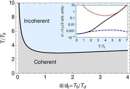
To illustrate this behaviour, in the main part of Fig. 1 we plot the crossover temperature, shown separating the coherent and incoherent regimes, as a function of donor-acceptor separation. The divergence of $T_{c}$ at small $d$ implies that coherent dynamics can survive at elevated temperatures when strong fluctuation correlations suppress multi-phonon effects, consistent with recent experimental observations [7]. Further, the change in $T_{c}$ behaviour from small to large separations can provide information on the correlation length of the bath. Specifically, once the distance dependence of $T_{c}$ becomes weak there is no longer significant correlation between fluctuations at each site.

To give Fig. 1 a relevant experimental context, we now estimate $T_{0}$ and $T_{d}$ for two closely-spaced semiconductor QDs, as realized experimentally in Ref. [5], which could be brought into resonance by applying an external electric field. Typically, deformation potential coupling to acoustic phonons dominates exciton dephasing in such samples [20]. A simple model [31] allows an estimate of $A=0.032$ ps² in this case, implying $T_{0}\approx 9.6$ K. Taking $c=5110$ ms^-1 [20] and a dot separation $d=4.5$ nm [5], we find $T_{d}\approx 2.8$ K. Setting $V_{0}/k_{B}T_{0}=1$ and $d/d_{0}=T_{0}/T_{d}$ then implies the reasonable values $V_{0}\approx 0.8$ meV and $d_{0}\approx 1.3$ nm [20], respectively. From Fig. 1 we then obtain a crossover temperature of $T_{c}\approx 30$ K, below which we expect the energy transfer dynamics to display signatures of coherence. In fact, in Ref. [5] temperatures of around $4-40$ K were explored, which should therefore be a promising range over which to observe both coherent and incoherent transfer dynamics in QD samples.

Off-resonant - It is also important to examine the dynamics when the donor and acceptor are far off-resonant with each other, such that $V_{F}/\epsilon\ll 1$. This can occur quite naturally, for example in QD samples due to the nature of their growth. Furthermore, the recent weak-coupling theory of Ref. [20] predicts a single transfer rate in the off-resonant regime, and thus provides a means to assess the validity of our theory in this limit. As in the resonant case, we derive a set of Bloch equations from Eq. (27), this time expanding the resulting expressions to second-order in $V_{F}/\epsilon$. We find system dynamics well approximated by $\langle\sigma_{z}\rangle_{t}\approx e^{-\Gamma t}-(1-e^{-\Gamma t})\tanh{(\beta\epsilon/2)}$, describing incoherent energy transfer from the initially excited donor to the acceptor at a rate $\Gamma=V_{F}^{2}\frac{(1+2N(\epsilon))}{(1+N(\epsilon))}(\gamma_{x}(\epsilon)+\gamma_{y}(\epsilon))$. Taking the weak coupling limit of $\Gamma$ by retaining only single-phonon terms, we find $\tilde{\Gamma}\approx(4\pi\tilde{V}_{R}^{2}/\epsilon^{2})J(\epsilon)(1-F(\epsilon,d))\coth{(\beta\epsilon/2)}$, consistent with Ref. [20] once renormalisation of $V_{R}$ has been included there. In the opposite, high temperature limit ($k_{B}T\gg\epsilon$), we again find $\langle\sigma_{z}\rangle_{t}\approx e^{-\Gamma t}$, with $\Gamma=\Gamma_{1}$ of Eq. (11).

Summary - I have presented an analytical theory of excitation transfer in a correlated environment, showing that for resonant donor and acceptor, a crossover from coherent to incoherent transfer is expected as multi-phonon effects begin to dominate. The theory outlined here opens up intriguing possibilities for further study of the role of coherence in the transfer dynamics of larger arrays, such as photosynthetic complexes [17, 18, 19]. For example, it enables one to address the important question of how the transfer efficiency changes in such systems when crossing from the coherent to incoherent regime.

I am very grateful to A. Olaya-Castro, S. Bose, and A. M. Stoneham for useful discussions. I am supported by the EPSRC, Griffith University, and the Australian Research Council Centre for Quantum Computer Technology.

References

- [1] T. Foerster, Discuss. Faraday Soc. 27, 7 (1959); D. L. Dexter, J. Chem. Phys. 21, 836 (1953).
- [2] T. F. Soules and C. B. Duke, Phys. Rev. B 3, 262 (1971).
- [3] S. Rackovsky and R. Silbey, Mol. Phys. 25, 61 (1973).
- [4] S. A. Crooker et al., Phys. Rev. Lett. 89, 186802 (2002).
- [5] B. D. Gerardot et al., Phys. Rev. Lett. 95, 137403 (2005).
- [6] D. Kim et al., Phys. Rev. B 78, 153301 (2008).
- [7] E. Collini and G. D. Scholes, Science 323, 369 (2009).
- [8] T. Renger, V. May, and O. Kühn, Phys. Rep. 343, 137 (2001).
- [9] R. van Grondelle and V. I. Novoderezhkin, Phys. Chem. Chem. Phys. 8, 793 (2006).
- [10] H. Lee, Y.-C. Cheng, and G. R. Fleming, Science 316, 1462 (2007).
- [11] G. S. Engel et al., Nature 446, 782 (2007).
- [12] Y.-C. Cheng and G. R. Fleming, Annu. Rev. Phys. Chem. 60, 241 (2009).
- [13] H.-P. Breuer and F. Petruccione, The Theory of Open Quantum Systems (Oxford University Press, 2002).
- [14] J. B. Gilmore and R. H. McKenzie, Chem. Phys. Lett. 421, 266 (2006).
- [15] J. A. Leegwater, J. Phys. Chem. 100, 14403 (1996); A. Kimura and T. Kakitani, J. Phys. Chem. A 111, 12042 (2007).
- [16] Z. G. Yu, M. A. Berding, and H. Wang, Phys. Rev. E 78, 050902(R) (2008).
- [17] Y. C. Cheng and R. J. Silbey, Phys. Rev. Lett. 96, 028103 (2006).
- [18] A. Olaya-Castro et al., Phys. Rev. B 78, 085115 (2008).
- [19] M. Mohseni et al., J. Chem. Phys. 129, 174106 (2008); M. B. Plenio and S. F. Huelga, New J. Phys. 10, 113019 (2008); P. Rebentrost, M. Mohseni, and A. Aspuru-Guzik, J. Phys. Chem. B 113, 9942 (2009).
- [20] E. Rozbicki and P. Machnikowski, Phys. Rev. Lett. 100, 027401 (2008).
- [21] M. Yang and G. R. Fleming, Chem. Phys. 282, 163 (2002).
- [22] W. M. Zhang et al., J. Chem. Phys. 108, 7763 (2002).
- [23] H. Sumi, J. Phys. Chem. B 103, 252 (1999); G. D. Scholes and G. R. Fleming, J. Phys. Chem. B 104, 1854 (2000); S. Jang, M. D. Newton, and R. J. Silbey, Phys. Rev. Lett. 92, 218301 (2004).
- [24] A. Würger, Phys. Rev. B 57, 347 (1998).
- [25] S. Jang et al., J. Chem. Phys. 129, 101104 (2008).
- [26] V. M. Kenkre and R. S. Knox, Phys. Rev. B 9, 5279 (1974); T. Renger and R. A. Marcus, J. Chem. Phys. 116, 9997 (2002); M. Thorwart et al., Chem. Phys. Lett. 478, 234 (2009).
- [27] I. Sinaysky, F. Petruccione, and D. Burgarth, Phys. Rev. A 78, 062301 (2008).
- [28] A. O. Govorov, Phys. Rev. B 71, 155323 (2005).
- [29] R. J. Silbey and R. A. Harris, J. Chem. Phys. 80, 2615 (1984).
- [30] See supplementary information for the master equation dervation.
- [31] A. Nazir, Phys. Rev. B 78, 153309 (2008).
I Supplement: Derivation of the master equation
In this supplement, I outline the derivation of the master equation (Eq. (1) of the paper) used to describe the donor-acceptor energy transfer dynamics in the single-excitation subspace.
As in the paper, we write the polaron-transformed Hamiltonian within the single excitation subspace as
- [1] H.-P. Breuer and F. Petruccione, The Theory of Open Quantum Systems (Oxford University Press, 2002).
- [2] A. Würger, Phys. Rev. B 57, 347 (1998).