Classical Processing Requirements for a Topological Quantum Computing System.
Abstract
Dedicated research into the design and construction of a large scale Quantum Information Processing (QIP) system is a complicated task. The design of an experimentally feasible quantum processor must draw upon results in multiple fields; from experimental efforts in system control and fabrication through to far more abstract areas such as quantum algorithms and error correction. Recently, the adaptation of topological coding models to physical systems in optics has illustrated a possible long term pathway to truly large scale QIP. As the topological model has well defined protocols for Quantum Error Correction (QEC) built in as part of its construction, a more grounded analysis of the classical processing requirements is possible. In this paper we analyze the requirements for a classical processing system, designed specifically for the topological cluster state model. We demonstrate that via extensive parallelization, the construction of a classical “front-end” system capable of processing error correction data for a large topological computer is possible today.
pacs
03.67.Lx, 07.05.WrI Introduction
The design and construction of a feasible large scale quantum computing system has been a highly sought after and long term goal of quantum information science ever since the first physical system proposals were made in the mid 1990’s [1, 2, 3, 4, 5, 6, 7, 8, 9, 10]. While experimental advances in quantum computing have been pronounced [11, 12, 13, 14, 15, 16, 17, 18, 19] we are not yet at the stage where we can faithfully claim a multi-million qubit device is just around the corner.
Nevertheless, in order for experimental progress to be made, the fundamental theoretical building blocks for a large scale computer need to be firmly in place. This theoretical development is not restricted to the discovery of new protocols for computation, algorithms or error correction but it also includes the architectural engineering of future computers.
While there has been steady progress over the past 15 years on designing novel and (more importantly) experimentally feasible large scale processor architectures, the complication of implementing appropriate and efficient error correction procedures and designing systems which can trivially be scaled to the level of a “programmable”, multi-task computer is still a daunting and often neglected area of research.
Recently, the introduction of theoretical ideas such as topological cluster state quantum computing (TCQC) [20, 21, 22] and the single photon optical architecture [23, 24] gives us an idea of what a truly large scale device may possibly look like. The modular design of the cluster preparation network, and the measurement based nature of the computational model, gives this design something that other architectures arguably lack, a strictly modular scaling of the entire computer.
While the design introduced in Refs. [23, 25] is not necessarily the optimal way to construct a large scale quantum computer, it does contain several key elements, easing the conceptual design of a large scale computer. For example:
- 1.
Utilizing a computational model that is fundamentally constructed from error correction, rather than the implementation of codes on top of an otherwise independent computational model.
- 2.
- 3.
Employing a computational model exhibiting high fault-tolerance thresholds [20], which relieves the pressure on experimental fabrication and control.
- 4.
Utilizing a measurement based model for computation [27]. By employing a measurement based computational model, the quantum component of the computer is a simple state preparation network. Therefore, programming such a device is a problem of classical software, not of hardware.
These properties, as well as others, allowed us to consider the structure of an extremely large mainframe-type device. In Ref. [25], the quantum analogue of high performance computing was examined. The conceptual scalability of the optical architecture allowed us to examine the operating conditions, physical structure and resource costs of a computer employing extensive topological error correction to the level of 2.5 million logical qubits.
In addition to examining the implementation of a large scale TCQC, the nature of the topological model also allows for a more concrete discussion on an often neglected, but important aspect of quantum information processing, namely what are the classical computational requirements of a large scale device? In this paper we attempt to answer this question.
There have been several broad investigations into the classical structure, design and operation of a large scale quantum computer [28, 29], but investigation into this topic is difficult. The primary obstacle in analyzing classical requirements is that the quantum architecture generally has to be specified. Since all classical processing is ultimately dependent on both the computational model employed at the quantum level and more importantly the error correction protocols utilized, a detailed analysis of the classical front end must wait for the design of the quantum processor.
In this paper we specifically analyze the classical front end requirements to perform active error correction on a 3D topological cluster lattice prepared by the photonic chip network. This analysis will be restricted to the classical system required to implement the underlying error correction procedures in the topological model, without the execution of an active quantum algorithm.
Although we present this analysis in the context of the optical network presented in Ref. [23], it should be stressed that this analysis is still highly relevant for any physical architecture employing the 2D or 3D topological model [30, 31, 21, 20, 32]. Our analysis demonstrates that with several optimizations of the classical processing and the ability to significantly parallelize classical error correction processing, the classical computational requirements for large scale TCQC are indeed within the capabilities of today’s processing technology.
Section II very briefly reviews the nature of the topological cluster model in order to fully specify what is required of the classical processing. Section III reviews the flowing nature of the preparation network, and how this relates to the optical measurement layer, and the first level of classical processing. In Section IV we overview the basic requirements of the classical network and how target processing rates are related to the clock cycle of the quantum network. In Section V we introduce classical benchmarking data for the minimum weight matching algorithm utilized for error correction and illustrate, given this data, how error correction processing can be parallelized over the entire computer. We conclude by illustrating how the parallelization of the classical processing allows, in principal, for the construction of a classical error correcting front end for large scale TCQC with classical processing technology available today.
II Topological Error Correction in the Optical Architecture
TCQC was first introduced by Raussendorf, Harrington and Goyal in 2007 [21, 20]. This model incorporates the ideas stemming from topological quantum computing introduced by Kitaev [33] and cluster state computation [27], leading to a very attractive computational model incorporating error correction by construction and exhibiting a high threshold error rate.
As with any measurement based computational model, computation proceeds via the initial construction of a highly entangled multi-qubit state. Fig. 1 illustrates the structure of the cluster. Each node in the cluster represents a physical qubit, initially prepared in the state, and each edge represents a controlled- entangling gate between qubits. This is the fundamental unit cell of the cluster, which repeats in all three dimensions.
Computation under this model is achieved via the consumption of the cluster along one of the three spatial dimensions [22] (simulated time). Logical qubits are defined via the creation of “holes” or “defects” within the global lattice and multi-qubit operations are achieved via braiding (movement of these defects around one another) as the cluster is consumed along the direction of simulated time. The specific details for computation under this model are not important for this discussion and we encourage the reader to refer to Refs. [20, 22] for further details. For this analysis, the effect of errors on a topological lattice is the important factor.
II.1 Error effects
Quantum errors in this model manifest in a very specific way. In Fig. 1, illustrating the unit cell of the cluster, we have illustrated six face qubits shown in red. If no errors are present in the system, measuring each of these six qubits in the or states ( basis) will return an even parity result. If we denote the classical result of these six measurements as , , then
| (1) |
This result is a consequence of the quantum correlations established in the preparation of the cluster. If the cluster is prepared perfectly, these six qubits are placed into a state that is a eigenstate of the operator
| (2) |
where is the Pauli bit-flip operator. The measurement of each of these six qubits in the basis will produce random results for each individual qubit. However the eigenvalue condition of this correlation operator guarantees the classical measurement results satisfy Eq. 1 in the absence of errors.
The remaining qubits in each unit cell are also measured in the basis, but their results are associated with the parity of cells within the dual lattice [Fig. 2]. This property of the cluster is not important for this discussion. What is important is that when no quantum algorithm is being implemented, every qubit is measured in the basis and is used to calculate the parity of their respective cells.
Due to the structure of this 3D cluster state, all error channels can effectively be mapped into phase errors (Pauli- operations applied to phyical qubits in the lattice which takes a state, ) or physical qubit loss [22]. These two distinct channels are processed slightly differently.
II.2 Error channel one: Phase errors
We first consider the effect of phase errors, which act to flip the parity of a cell of the cluster. As the Pauli operators and anti-commute, , if a phase error occurs to one of these six qubits the correlation condition of a cell will flip from a +1 eigenstate of the operator to a -1 eigenstate. If the correlation condition flips to a eigenstate of , the classical result of the six individual measurements also flips to an odd parity condition, i.e.
| (3) |
Errors on qubits on the boundary of each unit cell therefore flip the parity of the measurement result from even to odd. Note that the change of parity of any individual cell gives us absolutely no information regarding which one of the six qubits experienced the physical error.
The second important aspect of this structure is that any given qubit lies on the boundary of two cells in the cluster. If a given qubit experiences a phase error it will flip the parity result of the two adjacent cells. This allows us to detect which of the six qubits of a given cell experienced an error. If a single cell flips parity, we then examine the parity result of the six adjacent cells. Assuming that only one error has occured, only one of these six adjacent cells will have also flipped parity allowing us to uniquely identify the erred qubit.
If we now consider more than one error within the lattice, we no longer identify the location of individual errors but instead identify error chains. Fig. 3 from Ref. [22] illustrates. Here we have a 3D cluster consisting of a cube of cells with three error chains. The first chain is a single error which flips the parity of the two adjacent cells, the other two chains illustrate the effect of multiple errors. As the parity conditions are cyclical (mod 2), if two errors occur on the boundaries of a given cell the parity result will not change. Instead, the two cells at the endpoints of these error chains are the cells which flip parity.
Hence, in the TCQC model, it is not the locations of individual errors which are important but the endpoints of error chains. In fact, the symmetries of the cluster do not require us to identify the physical error chain corresponding to the detected endpoints. Once the endpoints of the chain are correctly identified all path of correction operators (Pauli operators which are applied to reverse detected errors) which connect the two endpoints are equivalent [20]. Hence, the goal of error correction in this model is to correctly “pair up” a set of odd parity cells such that the appropriate correction operators can be applied.
Undetectable errors in this model occur when chains become so long that they actually connect two boundaries of the lattice. If a physical error chain completely spans the lattice from one boundary to another then each individual cell experiences two physical errors and every cell remains in an even parity state. If the 3D lattice is not used for computation, these error chains are actually invariants of the cluster and hence have no effect. Once computation begins, information is stored by deliberately creating holes (or defects) in this lattice. These defects act as artificial boundaries and consequently error chains connecting defects to any other boundary (either other defects or the boundary of the lattice) are undetectable and cause logical errors on stored information.
From the standpoint of this investigation we are only concerned with performing active error correction on a defect free lattice. We will not be introducing information qubits into the cluster. Instead we will be examining the classical resources required to detect and correctly identify error chains in an otherwise perfectly prepared lattice.
This type of analysis is justified as information qubits are essentially regions of the 3D cluster that have simply been removed from the global lattice. Analyzing the classical requirements for the complete, defect free lattice therefore represents the maximum amount of classical data that needs to be processed for correction.
II.3 Error channel two: Qubit loss
The second major error channel is qubit loss. As we are motivated by the optical architecture introduced in Ref. [23], loss represents a significant error channel. Unlike other computation models for quantum information, the TCQC model can correct loss without additional machinery. Without going into the details, loss events can be modeled by tracing out the qubit that is lost from the system and replacing the qubit with the vacuum. Tracing out the lost qubit is equivalent to measuring the qubit in the or state (a basis measurement) with the result unknown. In principal, this type of error can be modeled as a standard channel, causing the parity of the respective cells to flip with a probability of 50%. However, since the qubit is no longer present, we can utilize the vacuum measurement to uniquely identify these error events.
Illustrated in Fig. 4 is the structure of a unit cell when one qubit is essentially measured out via loss. In this case, the boundary of a cell increases around the lost qubit. Instead of the parity conditions being associated with the six face qubits of a given cell, it extends to be the combined parity of the ten measurements indicated. As the loss event is detected via no “clicks” from the detector array, this result is corrected by now taking the parity of this larger structure and proceeding as before. Provided no other errors have occured, the parity of this larger boundary will be even, and any additional qubit errors will link this extended cell to a second end point with odd parity. Recent results, obtained in the context of the surface code [31, 32], have demonstrated a high tolerance to heralded loss events [34].
III The optical computer, a “flowing” network
As introduced in Ref. [23], optical TCQC can be performed by making use of a preparation network of photonic chips [26]. This network receives a stream of single photons (from a variety of appropriate sources) and ejects a fully connected topological cluster. As computation proceeds via the successive consumption of lattice faces along the direction of simulated time, the preparation network is designed to continuously prepare the lattice along this third dimension at a rate equal to the rate of consumption by the detector layer. Fig. 5 illustrates the basic design.

Photons are continuously injected into the rear of the preparation network, ideally from appropriate on-demand sources. Each photon passes through a network of four photonic chips, which act to link them together into the appropriate 3D array. Each photonic chip operates on a fundamental clock cycle, , and each chip in the network operates in a well-defined manner, independent of the total size of the network [23]. In total, a single photon entering the network at will exit at , after which it can be measured by the detector banks.
Each photonic chip acts to entangle a group of five photons into an appropriate state such that the parity condition for each cell is satisfied. After each group of five photons passes through an individual chip, a single atomic system contained within each chip is measured and reinitialized, projecting the relevant group of 5-photons into an entangled state. The result of this atomic measurement is fed forward to the classical processing layer in order to define a set of initial correlation conditions. The cluster is defined such that Eq.1 is satisfied for all cells. However, the preparation network does not automatically produce these correlation conditions. Depending on the measurement results of the atomic systems contained within each photonic chip, approximately 50% of cells within the lattice will be prepared with an initial parity condition that is odd. This can, in principal, be corrected to be even for all cells by applying selective single qubit rotations dependent on the atomic readout results, but this is unnecessary. The initial parity results from the preparation network are simply recorded, endpoints of error chains are then identified with cells that have changed parity from this initial state.
As one dimension of the topological lattice is identified as simulated time, the total 2D cross section defines the actual size of the quantum computer. Defects, regions of the cluster measured in the basis, are used to define logical qubits and are kept well separated to ensure fault tolerance. The 2D cross section is then continually teleported, via measurement, to the next successive layer along the direction of simulated time allowing an algorithm to be implemented (in a similar manner to standard cluster state computation [27]).
In Fig. 6 we illustrate the structure of the detection system. For the sake of simplicity, we are assuming that the basis states for the qubits are photon polarization, and , hence the detection system consists of a polarizing beam splitter (PBS) and two single photon detectors. A given unit cell flows through a set of nine optical lines such that the relevant parity is given by,
| (4) |
where is the detection result of detector at time . This result defines the parity of the cell in the lattice. Loss events would result in neither detector firing, at which point the calculation of Eq. 4 would be redefined based on the loss event to calculate the parity of the boundary around this lost qubit.
The results of all the detection events are fed directly from the detectors into the first classical processing layer. This layer calculates Eq. 4 and passes the result forward to the subsequent processing layer if it differs from the initial parity. This general structure extends across the entire 2D cross section of the lattice with parities repeatedly calculated for each unit cell that flows into the detection system.
IV Classical Processing requirements
Illustrated in Fig. 7 is the layer structure of the classical processing for topological error correction. In total there are four stages, parity calculation, tree creation, minimum weight matching, and the quantum controller.
As this analysis is only considering the classical requirements for base level error correction processing, we will not discuss the structure for the quantum controller. This top-level processor will be responsible for the application of active quantum algorithms on the topological lattice, given inputs from both a quantum algorithm compiler, and error data outputted from the correction processors. In the future, we will be examining the requirements for this top level processor, but for now we omit details regarding its structure and operation.
The error correction in this model requires identifying all cells which have changed parity and reliably identifying pairs of parity changes associated with a physical error chain. In order for error correction to be effective, we assume a standard, stochastic, qubit error model. As all standard error channels (all errors except qubit loss) can be mapped under the topological model to phase errors [20, 22], we can, without loss of generality, assume that each qubit experiences a phase error, , with probability . Therefore, a stochastic hierarchy exists with respect to longer error chains.
As the probability of a single phase error is given by , the probability of an error chain is . Therefore, for a given set of parity results, the most likely set of physical errors producing the classical measurement pattern is the set of end point pairings where the total length of all connections is minimized.
Classical results stemming from the detection layer are used to calculate the parity for all unit cells for some total volume. The co-ordinates of all cells which have experienced a parity flip are stored in a classical data structure. Minimum weight matching algorithms [35, 36, 37, 38] are then used to calculate likely error chains corresponding to the detected endpoints. Once chains are calculated, the Pauli frame (the current eigenvalue condition for all cells relative to their initial state) of the computation, within the quantum controller, is updated with the new error information.
The frequency of error correction in the lattice is dictated by the application of the non-Clifford gate
| (5) |
This gate is required to generate a universal set of operations [39], and in the topological model is achieved via the injection of multiple, low fidelity, singular ancilla, magic-state distillation [40, 41] and the application of teleportation protocols with information qubits. In order to successfully apply logical gates, error information must be obtained for the qubit undergoing the teleported gate prior to application of the correction. Fig. 8 illustrates the teleportation protocol to implement an rotation. If a logical error exists on the state prior to teleportation, the condition
| (6) |
implies that this error must be known before teleporting the rotation . If the error is detected after teleportation, the conjugate rotation will actually be applied. Therefore, the classical processing of the minimum weight matching algorithm will have to occur at a comparable rate to the logical gate rate of the preparation network to ensure up-to-date error information for all logical qubits is available when teleported gates are applied.
As detailed in Ref. [42], the clock cycle of the preparation network can vary from nanoseconds to microseconds, depending on the system utilized to construct the photonic chip. Hence our goal in this investigation is to determine, for a given failure probability of the quantum component of the computer, how quickly the network be operated such that all classical processing can be performed utilizing today’s technology.
V Layers two and three: Minimum weight matching
Calculating the minimum weight matching of the classical parity data stemming from the first layer of the classical processing network is the essential requirement for error correction in the topological model. The parity processing layer is designed to simply output co-ordinate tuples for all parity changes in the lattice to this next layer. The relevant question is, can the minimum weight processing of this data be performed over a large volume of the cluster in a comparable time frame to the quantum preparation network?
V.1 Minimum Weight Matching benchmarking
Classical algorithms for determining the minimum weight matching of a connected graph are well known with a run-time polynomial in the total number of nodes [37, 38]. Such algorithms are derived from the original Edmonds’ Blossom algorithm [36] and for our benchmarking tests we have used Blossom V [38]. However, due to the nature of our problem, there are several adaptations that can be made to optimize the algorithm further.
Typical minimum weight matching algorithms accept a list of co-ordinates, , and of weighted edges (in this case, lattice separation between nodes) such that the corresponding graph is completely connected. The output is then a list of edges such that every node is touched by exactly one edge and the total weight of the edges is a minimum. For the purposes of TCQC we can optimize by considering the specifics of the problem.
Due to the stochastic hierarchy of errors in the qubit model, and the assumption that the operational error rate of the computer is low, , the most likely patterns of errors are simply sets of sparse single errors causing two adjacent cells to flip parity. The probability of obtaining longer and longer errors chains is increasingly unlikely.
Therefore, for a given volume of classical parity results, erred cells will tend to be clustered into small groups, as illustrated in Fig. 9. Additionally, we can consider the computational lattice structure. Fig. 10, taken from Ref. [23], illustrates the 2D cross-section of the cell structure once logical qubits are defined.
In this example, defects are separated from each other (and from the edge of the lattice) by a total of 16 cells. Logical errors occur when error chains connect two boundaries in the cluster. If an error chain spans more than 8 cells, the correction inferred from the endpoints is likely to be incorrect, resulting in defects connected by a chain of errors - a logical error.
This allows us to set a maximum edge length that is allowed between connections in the minimum weight matching algorithm. Instead of creating a completely connected graph structure from the classical data, we instead create multiple smaller subgraphs, with each subgraph having no connections of weight greater than a maximum edge parameter . As the separation and circumference of defects within the lattice determines the effective distance of the quantum code can safely be chosen such that . This approximation ensures that all error chains throughout the lattice with a weight are connected within the classical processing layer. This classical approximation is defined to fail if a single length error chain occurs during computation. This is much less likely than failure of the code itself which can occur as the result of numerous, not necessarily connected, arrangements of errors.
It should be noted that this approximation does not neglect all error chains longer than . However, the classical error correction data has no knowledge regarding the actual path an error chain has taken through the lattice. The approximation neglects all error chains with endpoints separated by cells.
By making this approximation, we speed up the classical processing for minimum weight as, on average, the algorithm will be run on a very sparse graph structure.
V.2 Classical simulations as a function of total cluster volume and code-distance.
Given the above classical approximation, we have benchmarked the Blossom V algorithm [38] as a function of the total volume of the cluster for various distances of the quantum code, and hence .
In order to investigate the classical processing requirements of the system, we will assume a physical error rate of the quantum computer. As with previous investigations into this system we will be assuming, throughout this discussion, that the quantum computer operates at a physical error rate of [23, 25] and the fault-tolerant threshold is [20].
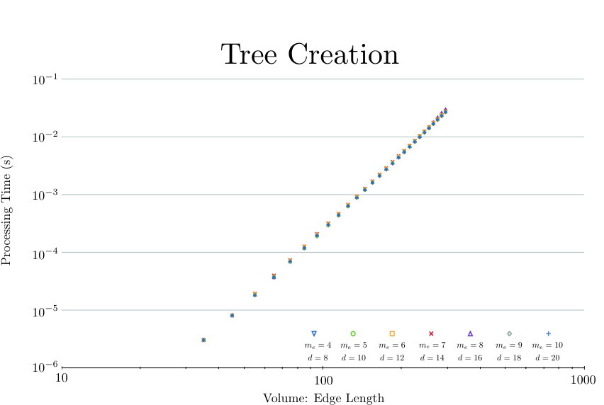
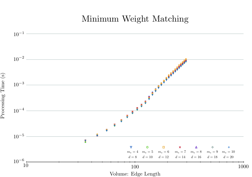
Given this base assumption, Figs. 11 and 12 examine the processing time of the modified Blossom V algorithm run on a MacBook Pro (technical details of this computer are summarized in Appendix. A). For various volume sizes, , from to cells, random single qubit errors were generated with a probability of . The processing time for each value of was examined for different distance quantum codes and hence different values of the approximation parameter, . A list of cell co-ordinate tuples, , corresponding to the endpoints of error chains (cells with changed parity) was constructed. This list is the input to the classical processor as, in practice, it would be provided directly by the hardware.
The tuple data was then processed in two stages. In the first stage, which we denote as the tree creation layer, an 8-way sort/search tree was created from the tuple information and then used to generate a list of connections (edges) between cells and their distances (weights) [Fig. 11]. The second stage of the simulation applied the Blossom V minimum weight matching algorithm to the generated sparse graph structures [Fig. 12]. The benchmarking data was taken using runs per data point.
For each cluster volume, code distances , corresponding to were simulated. For both the tuple tree creation and the minimum weight matching, Figs. 11 and 12 illustrate that the approximation parameter, , does not significantly alter the total simulation time and that for a given (), tree creation and minimum weight matching take a similar amount of time.
V.3 Parallelizing the algorithm
The numerical simulations shown in Figs. 11 and 12 clearly illustrate that the minimum weight matching subroutine cannot be run over the entire lattice used for TCQC. As a rough estimate, a mainframe device such as the one introduced in Ref. [25] consists of a lattice cross section measuring unit cells. Clearly in order to achieve classical processing speeds of the order of microseconds (for any distance topological code), either the classical fabrication of the processing equipment must allow for at least a 10–15 order of magnitude speed up from a standard Laptop or the application of the tree creation and minimum weight subroutines must be highly parallelized.
Due to the approximation made to the Blossom V algorithm, parallelizing the classical processing is possible. The approximation to the subroutine prohibits the establishment of graph connections between two cluster cell co-ordinates separated by a distance . In Fig. 13 we illustrate the relative frequency of different sized connected components within the lattice at an error probability of , for . These simulations were performed using the Floyd-Warshall algorithm [43, 44] obtained for a volume region of , with statistical runs (resulting in approximately connected components in total). In these simulations, the size of each connected component in the lattice, , does not represent the longest path through the graph. Instead it represents the physical edge length through the cluster of a cube of sufficient size to fully contain each connected component. In Appendix B we provide additional simulations showing the distribution of connected components within the cluster to assist in the explanation of Fig. 13.

Parallelizing the minimum-weight matching procedure requires subdividing up a large volume of the cluster into smaller regions such that each instance of the tuple tree creation and the minimum weight algorithms faithfully return the same results as processing the entire volume (up to the failure probability of the computer). In Fig. 13 we provide an approximate scaling of the decay of each curve, representing the volume independent relative frequency of connected component with a linear size, , in the cluster. In order to parallelize classical processing, two regions are defined. Fig. 14a. illustrates.
The inner volume defines the minimum weight processing region while the outer volume, with an edge length of the inner volume, defines the tree creation processing region. During tuple tree creation, if any connected component contains at least one vertex within the inner volume it is sent to independent instances of minimum weight matching. Provided that the edge length of these regions are large enough, then any connected component with at least one vertex in the inner volume will be fully contained within the outer volume with high probability.
To determine the size of these processing regions we utilize the decay of the curves in Fig. 13. The probability of failure when parallelizing classical processing should be approximately the same as the failure probability of the quantum computer itself. In order to determine these failure probabilities, we consider the volume of the cluster required to perform a logical CNOT operation as a function of . Fig. 10 illustrates the logical structure of the lattice. Each logical qubit cell in the cluster consists of a cluster cross-section measuring cells. A CNOT gate requires 4 logical cells and the depth through the cluster required to perform the gate is cells [20]. Hence the total cluster volume for a CNOT operation is cells.
The failure probability of the quantum computer during a logical CNOT is approximately,
| (7) |
where,
| (8) |
is the probability of failure for a single logical qubit a single layer thick, with a fault-tolerant threshold of , and is the number of such layers of the cluster that need to be consumed to perform a logical CNOT operation.
Given the failure rate of the quantum computer, we utilize the data from Fig. 13 to determine the edge length of a volume large enough to encapsulate all connected components with a probability approximately equal to Eq. 7. As Fig. 13 represent relative frequencies (the probability of a connected component of size , relative to a connected component of size one) we scale by the number of isolated errors expected in a cluster volume required for a CNOT. Hence,
| (9) |
where the factor of 6 comes from the 6 independent qubits per unit cell of the cluster. Eq. 9 is then solved for giving,
| (10) |
where are the scaling parameters shown in Fig. 13.
The values of for and the probabilities of the logical CNOT failure and equally the probability of a connected component of size greater than are shown in Tab. 1.
| CNOT failure | |||
|---|---|---|---|
| 4 | 10 | ||
| 5 | 15 | ||
| 6 | 23 | ||
| 7 | 32 | ||
| 8 | 44 | ||
| 9 | 62 | ||
| 10 | 81 |
In Tab. 1 we give the size of the processing regions for parallelizing both the tuple tree creation and minimum weight matching processes such that the probability of any connected component within the inner region unbounded by the boundary of the outer region is approximately the same as the failure rate of the quantum computer. The value therefore sets the edge length of the inner and outer volume regions.
Using this estimate, the tree creation layer becomes an interlaced network, with each individual instance of tree creation operating over a volume of .
As we can neglect larger connected components (which occur with probability roughly equal to the probability of quantum failure), any connected component that contains at least one vertex within a central volume will be fully contained within the outer volume of . The central volume represents the region that is sent to separate instances of the minimum weight matching algorithm. The tree creation layer is interlaced such that each of the central volumes touch but do not overlap.
This processing structure ensures that multiple parallel instances of minimum weight matching will produce identical results to an individual instance of minimum weight matching run over the entire volume. As the tree creation layers are interlaced, tree structures that cross the boundaries of two inner volumes regions will be sent to two independent instances of minimum weight matching. After processing, these duplicate results will simply be removed from the final error list.
We can now combine the results from Tab. 1 with the simulation data of Figs. 11 and 12 to determine the maximum size and speed of a quantum computer such that error correction data can be processed sufficiently quickly. Fig. 14b. illustrates how error correction data is collected as qubits along the third axis of the cluster are sequentially measured. As the tuple tree creation processing layer consists of an interlaced set of cubes, two thirds of the data for any given volume is taken from the previously collected results while the final one third consists of newly collected data. Therefore the processing “window” available for each instance of the tuple tree creation (and hence each instance of minimum weight matching associated with each tree creation volume) is the time required to collect this new data.
The optical network illustrated in Sec. III has each parity calculation from the detector banks, for each unit cell, occurring over three successive cluster faces and, in the absence of loss, occur every 2, where is the separation period of photons (the quantum clock rate). Tree creation from the parity tuples for a given volume element utilizes the last tuple information from the previous instance of tree creation and must store the same amount for use in the next tree creation subroutine. Parity tuple tree creation processing is repeated for each volume every seconds.
Taking the simulation data from Fig. 11 (as tuple tree-creation is the slower of the two processes), the fastest clock cycle, can be calculated for each value of as,
| (11) |
where is the processing time as a function of the edge length of the processing volume, , shown in Fig. 12. The results are shown in Tab. 2.
| CNOT failure | “window”, | CNOT operating Freq. | Processing instances / Logical qubit, (I) | |||
| 4 | 10 | 0.06 | 19 | 105 kHz | 8.7 | |
| 5 | 15 | 0.28 | 31 | 18 kHz | 5.3 | |
| 6 | 23 | 1.1 | 46 | 4 kHz | 3.4 | |
| 7 | 32 | 3.2 | 64 | 1 kHz | 2.4 | |
| 8 | 44 | 9.3 | 87 | 0.3 kHz | 1.7 | |
| 9 | 62 | 28 | 124 | 0.1 kHz | 1.0 | |
| 10 | 81 | 68 | 162 | 37 Hz | 0.77 |
The last column in Tab. 2 calculates the total number of processing instances required per logical qubit in the computer. This is calculated as the ratio of the cross-sectional area of a logical qubit to the cross-sectional area of the minimum weight matching processing volume.
| (12) |
the factor of 4 is introduced since each instance of minimum weight matching has an associated tuple tree creation process and that primal and dual lattice error correction is performed independently giving another factor of two. As the size of the quantum computer increases (increasing ) this ratio decreases as the scaling of is approximately .
While the total size and speed of a topological quantum computer will ultimately be governed by the experimental accuracy in constructing each quantum component, the results shown in Tab. 2 are promising. Assuming that quantum fabrication can reach and accuracy of , current classical technology is quite sufficient to process error correction data for a large range of computer sizes. The logical failure rate of the CNOT gate approximately defines the size of the computer, , where is the number of logical qubits in the computer and is the number of logical time steps in a desired quantum algorithm (note that the application of non-clifford gates will lower this effective size further). Even for a small topological computer ( has sufficient protection for 1000 logical qubits running an algorithm requiring approximately time steps) less than ten classical processing instances are required per logical qubit, a quantum network run at MHz with a logical CNOT operating frequency of kHz.
The classical processing power utilized in this investigation is clearly not specially designed for the task of operating a topological computer. Not only can we safely assume that classical processing power will increase before the advent of a large topological computer, but the design and implementation of both specialized hardware and more optimal coding should also result in significant increases in the achievable operational frequency of the quantum network and logical gates. More recent analysis has suggested that possible operational frequency of the quantum network could reach the MHz level [45]. In this case, if classical processing could result in a 2-3 order of magnitude speed up when moving to optimized hardware and software, current classical technology would be sufficient for a quantum computer capable of a logical error rate and a logical CNOT frequency of MHz.
VI Observation and Conclusions
In this work we have focused exclusively on the classical requirements to perform the underlying error correction processing for the network. As the error correction procedures can be thought of as the base-level processing, the development of an appropriate quantum controller system is an obvious next step. This higher level classical controller will essentially be responsible for the following,
- 1.
The compilation of a user-designed quantum circuit into an appropriate measurement sequence on a topological cluster.
- 2.
Direct control of quantum components within the measurement system of the topological cluster in order to change the measurement basis for the photon stream.
- 3.
The dynamic allocation of cluster resources dependent on operational error rate. Specifically, the fundamental partitioning of the lattice into appropriately separated defect regions for logical qubit storage.
- 4.
Accepting the data from the error correction processing layer to faithfully ensure accurate error correction is performed during computation.
- 5.
Dynamical restructuring of the topological lattice partitioning to allow for ancilla preparation for non-Clifford quantum gates, and optimization of logical qubit/qubit interactions for specific quantum subroutines.
This last point is one of the more interesting questions that can be addressed in this model. As we noted in the introduction, once the cluster lattice is prepared, data processing is performed via software. The structure of the topological lattice essentially allows for qubit/qubit interactions in a 2D arrangement [Fig. 10]. However, provided we have access to a large cluster lattice, we can envisage the dynamical creation of data pathways and “flying defects” in order to speed up specific quantum subroutines. This could lead to some extremely interesting avenues of investigation in software control and optimization of a TCQC architecture.
This analysis has demonstrated that the classical error correction requirements necessary to construct an optical quantum computer based on topological cluster states is certainly feasible given today’s technology. We have illustrated how minimum weight matching, required to process error data from the topological mainframe, can be optimized in such a way to allow for a massively parallelized processing network that can process information for large topological clusters.
These results are very encouraging. As with the quantum preparation network, the classical front end can also be constructed in a modular manner. As the quantum preparation network is increased in sized via the addition of more photonic chips, the classical processing network is also expanded in a similar way. Parity check processors, tuple tree creation processors and minimum weight matching processors are also linked into a pre-existing network as its size expands. The results of this investigation give us a very optimistic outlook on the viability of the topological model as a possible avenue to achieve truly large scale quantum computation.
VII Acknowledgments
We would like to thank Rod Van Meter, Ashley Stephens, and Zac Evans for helpful discussions. We acknowledge the support of MEXT, JST, HP and the EU project HIP and the support of the Australian Research Council, the Australian Government, and the US National Security Agency (NSA) and the Army Research Office (ARO) under contract number W911NF-08-1-0527.
Appendix A Technical Specifications for simulations.
The technical specifications to the computer used in benchmarking simulations are summarized below.
| Process | Benchmark |
|---|---|
| Floating Point Basic | 3.1Gflop/s |
| vecLib FFT | 3.5 Gflop/s |
| Memory Fill | 6.2 GB/s |
Appendix B Simulations of graph sizes for cluster errors.
The simulations shown in Fig. 13 illustrate the distribution of the largest physical distance through the cluster (in a single spatial dimension) between any two nodes for each connected component for graph structures established using the approximation detailed in the main text. The following results illustrate the structure of this distribution in more detail.
References
- [1] J. Cirac and P. Zoller, Phys. Rev. Lett. 74, 4091 (1995).
- [2] D. Cory, A. Fahmy, and T. Havel, Proc. National Academy of Science 94, 1634 (1997).
- [3] N. Gershenfeld and I. Chuang, Science 275, 350 (1997).
- [4] B. Kane, Nature (London) 393, 133 (1998).
- [5] D. Loss and D. DiVincenzo, Phys. Rev. A. 57, 120 (1998).
- [6] E. Knill, R. Laflamme, and G. Milburn, Nature (London) 409, 46 (2001).
- [7] J. Mooij, T. Orlando, L. Levitov, L. Tian, C. van der Wal, and S. Lloyd, Science 285, 1096 (1999).
- [8] Y. Nakamura, Y. A. Pashkin, and J. Tsai, Nature (London) 398, 786 (1999).
- [9] ARDA, Quantum information science and technology roadmap project, http://qist.lanl.gov (2004).
- [10] P. Kok, W. Munro, K. Nemoto, T. Ralph, J. Dowling, and G. Milburn, Rev. Mod. Phys. 79, 135 (2007).
- [11] I. Chiorescu, Y. Nakamura, C. Harmans, and J. Mooij, Science 299, 1869 (2003).
- [12] T. Yamamoto, Y. A. Pashkin, O. Astafiev, Y. Nakamura, and J. Tsai, Nature (London) 425, 941 (2003).
- [13] J. Chiaverini, D. Leibfried, T. Schaetz, M. Barrett, R. Blakestad, J. Britton, W. Itano, J. Jost, E. Knill, C. Langer, et al., Nature (London) 432, 602 (2004).
- [14] H. Häffner, W. Hänsel, C. Roos, J. Benhelm, D. C. al kar, M. Chwalla, T. Körber, U. Rapol, M. Riebe, P. Schmidt, et al., Nature (London) 438, 643 (2005).
- [15] J. Gorman, D. Hasko, and D. Williams, Phys. Rev. Lett. 95, 090502 (2005).
- [16] T. Gaebel, M. Domhan, I. Popa, C. Wittmann, P. Neumann, F. Jelezko, J. Rabeau, N. Stavrias, A. Greentree, S. Prawer, et al., Nature Physics (London) 2, 408 (2006).
- [17] R. Hanson, F. Mendoza, R. Epstein, and D. Awschalom, Phys. Rev. Lett. 97, 087601 (2006).
- [18] M. G. Dutt, L. Childress, L. Jiang, E. Togan, J. Maze, F. Jelezko, A. Zibrov, P. Hemmer, and M. Lukin, Science 316, 1312 (2007).
- [19] J. O’Brien, G. Pryde, A. White, T. Ralph, and D. Branning, Nature (London) 426, 264 (2003).
- [20] R. Raussendorf, J. Harrington, and K. Goyal, New J. Phys. 9, 199 (2007).
- [21] R. Raussendorf and J. Harrington, Phys. Rev. Lett. 98, 190504 (2007).
- [22] A. Fowler and K. Goyal, Quant. Inf. Comp. 9, 721 (2009).
- [23] S. Devitt, A. Fowler, A. Stephens, A. Greentree, L. Hollenberg, W. Munro, and K. Nemoto, New. J. Phys. 11, 083032 (2009).
- [24] R. Ionicioiu and W. Munro, arxiv:0906.1727 (2009).
- [25] S. Devitt, W. Munro, and K. Nemoto, arxiv:0810.2444 (2008).
- [26] A. Stephens, Z. Evans, S. Devitt, A. Greentree, A. Fowler, W. Munro, J. O’Brien, and K. Nemoto, Phys. Rev. A. 78, 032318 (2008).
- [27] R. Raussendorf and H.-J. Briegel, Phys. Rev. Lett. 86, 5188 (2001).
- [28] R. V. Meter, quant-ph/0607065 (2006).
- [29] A. Steane, Quant. Inf. Comp. 7, 171 (2007).
- [30] S. Bravyi and A. Kitaev, Quant. Computers and Computing 2, 43 (2001).
- [31] E. Dennis, A. Kitaev, A. Landahl, and J. Preskill, J. Math. Phys. 43, 4452 (2002).
- [32] A. Fowler, A. Stephens, and P. Groszkowski, arxiv:0803.0272 (2008).
- [33] A. Kitaev, Russ. Math. Serv. 52, 1191 (1997).
- [34] T. Stace, S. Barrett, and A. Doherty, Phys. Rev. Lett. 102, 200501 (2009).
- [35] Y. Chu and T. Liu, Science Sinica 14, 139 (1965).
- [36] J. Edmonds, J. Res. Nat. Bur. Standards 71B, 233 (1967).
- [37] W. Cook and A. Rohe, INFORMS Journal on Computing, 11, 138 (1999).
- [38] V. Kolmogorov, Mathematical Programming Computation (2009), URL http://dx.doi.org/10.1007/s12532-009-0002-8.
- [39] M. Nielsen and I. Chuang, Quantum Computation and Information (Cambridge University Press, 2000), 2nd ed.
- [40] S. Bravyi and A. Kitaev, Phys. Rev. A. 71, 022316 (2005).
- [41] B. Reichardt, Quant. Inf. Proc. 4, 251 (2005).
- [42] S. Devitt, A. Greentree, R. Ionicioiu, J. O’Brien, W. Munro, and L. Hollenberg, Phys. Rev. A. 76, 052312 (2007).
- [43] R. Floyd, Comm. of the ACM 5, 345 (1962).
- [44] S. Warshall, Journal of the ACM 9, 11 (1962).
- [45] C.-H. Su, A. Greentree, W. Munro, K. Nemoto, and L. Hollenberg, Phys. Rev. A. 78, 062336 (2008).