Divergence of infinite-variance nonradial solutions to the 3d NLS equation
Abstract.
We consider solutions to the 3d focusing NLS equation such that and is nonradial. Denoting by and , the mass and energy, respectively, of a solution , and by the ground state solution to , we prove the following: if and , then either blows-up in finite positive time or exists globally for all positive time and there exists a sequence of times such that . Similar statements hold for negative time.
1. Introduction
The 3d focusing nonlinear Schrödinger equation (NLS) is
| (1.1) |
where and . We shall denote the initial data . The standard local theory in is based upon the Strichartz estimates (see Cazenave [1], Tao [20]), and asserts the existence of a maximal forward time such that . If , then it follows from the local theory that as , and we say that blows-up in finite forward time. If, on the other hand, , then we say that exists globally in (forward) time. In this case, the local theory gives us no information about the behavior of as . Analogous statements hold backwards in time. In fact, if solves NLS, then solves NLS, and thus, it suffices to study the forward-in-time case11 1 This is not to say that a given solution must have the same forward-in-time and backward-in-time behavior; however, if is real-valued, then ..
Solutions to (1.1) in satisfy mass, energy, and momentum conservation, given respectively by
There exists a ground state (minimal norm) solution to the (stationary) nonlinear elliptic equation
which is unique modulo translation and gauge symmetry. This is radial, smooth, positive, and behaves as for . It gives rise to a solution to (1.1) called the ground state soliton.
In Holmer-Roudenko [9], we proved that if , and , then blows-up in finite forward (and finite backward) time, provided that either (1) , that is, the initial data (and hence, the whole flow ) has finite variance, or (2) (and hence, the whole flow ) is radial. Moreover, it is sharp in the sense that solves NLS and does not blow-up in finite time. Via the Galilean transform and momentum conservation, if , this can be refined to the following: if and , then the above conclusions hold (see Appendix B for clarification). These results are essentially classical. The finite variance case follows from the virial identity [21], [6]:
and the sharp Gagliardo-Nirenberg inequality [22]. The radial case follows from a localized virial identity and a radial Gagliardo-Nirenberg inequality [19]. The radial case is an extension of a result of Ogawa-Tsutsumi [17], who proved the case . Martel in [13] showed that in the case of either finite variance or radiality assumptions can be relaxed to nonisotropic ones, namely, if (1) where , or (2) .
In this paper, we drop the additional hypothesis of finite variance and radiality and obtain the following conclusion:
Theorem 1.1.
Suppose , and . Then either blows-up in finite forward time or is forward global and there exists a sequence such that . A similar statement holds for negative time.
It is still possible, as far as we know, that a given solution satisfying the hypothesis might, say, blow-up in finite negative time but be global in forward time with the existence of a sequence such that . In other words, a given solution might have different behavior in forward and backward times.
The above remarks regarding the refinement for , by applying a Galilean transformation to convert to a solution with , apply in the context of Theorem 1.1 as well. In fact, we will always assume in this paper (see Appendix B for the standard details).
A result similar to Theorem 1.1 was obtained by Glangetas-Merle [5] for the case of (see also Nawa [16]). However, our proof is different in structure and uses a different form of concentration compactness machinery. Our proof is more akin to the proof of the scattering result we have in [9], [2], appealing to (suitable adaptations of) the profile decomposition results of Keraani [11], nonlinear perturbation theory based upon the Strichartz estimates, and rigidity theorems based upon the localized virial identity. Our scattering result was in turn modeled on a similar result by Kenig-Merle [10] for the energy-critical NLS equation. In his various lectures, Kenig refers to this scheme as the “concentration compactness–rigidity method” and discusses a “road map” for applying it to various problems. We believe that this method applied to prove Theorem 1.1 has more potential for generalization. In particular, it could perhaps provide an affirmative answer to:
Weak conjecture. Under the hypothesis of Theorem 1.1, either blows-up in finite forward time or as .
Strong conjecture. Under the hypothesis of Theorem 1.1, blows-up in finite forward time.
Why are we interested in removing the finite-variance hypothesis from our earlier result? The assumption might be considered unnatural on the grounds that blow-up is a local-in-space phenomenon and should not be dictated, in such a strong sense, by the size of the initial data at spatial infinity. In the case addressed in [9], the proof given via the virial identity actually provides, once the solution is scaled so that , an upper bound on the blow-up time , where is given as:
and
Here, is a constant depending on that diverges as . We carry out this classical argument in Prop. 3.1. This upper bound is actually an estimate for the time at which if were to continue to exist up to that time. However, numerics show that even if blow-up occurs at the origin, the variance actually does not go to zero at the blow-up time due to radiated mass ejected from the blow-up core, and thus, blow-up occurs before the time predicted by this method. This suggests that the full variance is not the correct quantity on which to base a blow-up theory. An analysis of the radial case using the radial Gagliardo-Nirenberg inequality (carried out in Prop. 3.3) reveals that there is an upper bound expressible entirely in terms of a spatially truncated version of as well as the proximity of to . Thus, the size of the initial variance does not appear at all, and can be thought of as measuring the degree and sign of quadratic phase.22 2 The relevance of quadratic phase seems very important from our numerics, see forthcoming paper [7]. We remark that in the 2d case it is exactly quantifiable via the pseudoconformal transformation. Theorem 1.1 might be considered the first step in assessing the relevance of the variance in blow-up theory of nonradial solutions, even though it is, unfortunately, nonquantitative.33 3 Another problem we face in the nonradial case is that of predicting the location of the blow-up. Nothing says that blow-up should occur at the origin, even if .
Another motivation is that there exist equations with less structure that NLS, such as the Zakharov system, for which the assumption of finite variance is not known to be of assistance in proving that negative energy solutions blow-up. Merle [14] proved using a localized virial-type identity that radial negative energy solutions of the 3d Zakharov system behave according to the conclusion of Theorem 1.1. No result is known for nonradial solutions (finite-variance or not) and it is conceivable that the concentration compactness methods of this paper might be of assistance in addressing this case. Even for the 3d NLS equation (1.1) itself, there are studies in the behavior of finite-time blow-up solutions, such as the divergence of the critical norm proved for radial solutions in Merle-Raphael [15], for which concentration compactness methods might enable one to remove the radiality assumption.
The paper is structured as follows. §2–6 are devoted to preparatory material; §7–9 are devoted the proof of Theorem 1.1. In §2, we review the dichotomy and scattering result we obtained in [9], [2]. In §3 we deduce some blow-up theorems for the virial identity and its localized versions – in the nonradial case, we are forced to assume an a priori uniform-in-time localization on the solution under consideration. In §4, we rewrite the variational characterization of the ground state from Lions [12] in a form that is more compatible with the scale-invariant perspective of this paper; this material is needed for §5. In §5, we carry out the base-case of the inductive argument that follows in §7–9. Under the assumption that Theorem 1.1 is false, we are able to construct a special “critical” solution that remains uniformly-in-time concentrated in . Such a solution would contradict the results of §3, and hence, cannot exist.
1.1. Acknowledgements
The second author would like to thank Patrick Gérard for discussions leading to the questions addressed in this paper and help in retrieving the reference [5]. J. H. is partially supported by a Sloan fellowship and NSF Grant DMS-0901582. S. R. is partially supported by NSF-DMS grant # 0808081.
2. Ground state and dichotomy
We begin by recalling a few basic facts about the ground state , the minimal mass solution of .
Weinstein [22] proved that the sharp constant of Gagliardo-Nirenberg inequality
| (2.1) |
is achieved by taking . Using the Pohozhaev identities
we can express as
| (2.2) |
The Pohozhaev identities also give:
| (2.3) |
Let
| (2.4) |
By (2.1), (2.2), and (2.3), we have
| (2.5) |
see Figure 1.

Suppose that . Then we have 2 cases:
- •
If , then there exist two solutions (see Figure 2) to
(2.6) - •
If , then there exists exactly one solution to (2.6).
By the local theory, there exist such that is the maximal time interval of existence for solving (1.1). Moreover,
with a similar statement holding if .
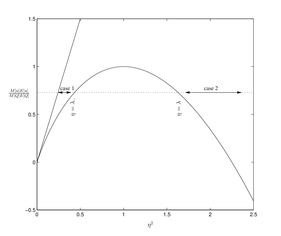
The following is a consequence of the continuity of the flow (see Figures 1–2). The proof is carried out in [9, Theorem 4.2].
Proposition 2.1 (dichotomy).
Let and be defined as above. Then exactly one of the following holds:
- (1)
The solution is global (i.e., and ) and
- (2)
The first case is only possible for .
Naturally, one can check the initial data (the value of ) to determine whether the solution is of the first or second type in Prop. 2.1. Note that the second case does not assert finite-time blow-up (this is the subject of this paper). In the first case, we proved in [9], [2] that more holds.
Theorem 2.2 (scattering).
If and the first case of Prop. 2.1 holds, then scatters as or . This means that there exist such that
| (2.7) |
Consequently, we have that
| (2.8) |
and
| (2.9) |
Let us justify (2.8)–(2.9) since they are not mentioned in [9], [2]. By (2.7), the Gagliardo-Nirenberg inequality, and mass conservation for the linear and nonlinear flows, we have
The statement in (2.8) then follows by the linear decay estimate and an approximation argument (to deal with the fact that ).44 4 As a result of this approximation argument, we lose the quantitative estimate of on the rate of decay. By (2.8), we have
Multiply by and use the Pohozhaev identities to obtain (2.9).
3. Virial identity and blow-up conditions
Now we turn our attention to the second case of Prop. 2.1. We begin by giving the classical derivation, using the virial identity, of the upper bound on the (finite) blow-up time under the finite variance hypothesis.
Proposition 3.1 (Finite-variance blow-up time).
Note that
and
As we remarked in the introduction, we feel that the dependence of on (or ideally a spatially truncated version of it) is quite natural, but the dependence on seems unsubstantiated, placing a very strong weight on the size of the solution at spatial infinity.
Proof.
The virial identity gives
By the Pohozhaev identities,
By definition of and ,
Since (and ), we have
Integrating in time twice gives
The positive root of the polynomial on the right-hand side is as given in the proposition statement. ∎
We next review the local virial identity. Let be radial such that
For define
| (3.1) |
Then direct calculation gives the local virial identity:
| (3.2) |
Note that
where, for suitable 55 5 Note that in the upper bound we do not need the term . This term was needed in the lower bound that was applied in the proof of the scattering theorem [2].
| (3.3) |
Using the local virial identity, we can prove a version of Prop. 3.1, valid without the assumption of finite variance but assuming that the solution is suitably localized in for all times. Define
Proposition 3.2 (Blow-up time for a priori localized solutions).
Let and and suppose that the second case of Prop. 2.1 holds (take to be as defined in (2.6)). Select such that , where is an absolute constant. Suppose that there is a radius such that for all , there holds . Define to be the scaled local variance:
Then blow-up occurs in forward time before (i.e., ), where
One could, in fact, define and obtain the same statement with a similar proof but a different Gagliardo-Nirenberg inequality.
Proof.
By the local virial identity and the same steps used in the proof of Prop. 3.1,
By the estimates (the first one is the exterior version of Gagliardo-Nirenberg)
| (3.4) |
and
| (3.5) |
applied to control the term, and using that , we obtain
The remainder of the argument is the same as in the proof of Prop. 3.1. ∎
For comparison purposes, we review the quantified proof of finite-time blow-up for radial solutions presented in [9].
Proposition 3.3 (Radial blow-up time).
Let and and suppose that the second case of Prop. 2.1 holds (take to be as defined in (2.6)). Suppose that is radial. Let
where is an appropriately large, but absolute, constant. Define to be the scaled local variance:
Then blow-up occurs in forward time before (i.e., ), where
We have that
where as (i.e., as ).
Proof.
We modify the proof of Prop. 3.2 only in (3.4) and (3.5) by using the radial Gagliardo-Nirenberg inequality [19] instead of (3.4)
and also
Then we have, for some absolute constant ,
We require that is large enough so that . Since increases as increases, and , we have
This gives
The restriction on in the proposition statement is such that
from which it follows that
The remainder of the argument is the same as in the proof of Prop. 3.1. ∎
4. Variational characterization of the ground state
For now, write (time dependence plays no role) in what follows in this section. The goal of this section is a variational characterization of the ground state stated below as Prop. 4.1. For the proof we will just show how it follows from scaling, the bounds depicted in Figure 1, and an existing characterization of appearing in Lions [12, Theorem I.2]. Prop. 4.1 will be one of the main ingredients in our treatment of the “near boundary case” in §5.
Proposition 4.1 (Variational characterization of the ground state).
There exists a function with as such that the following holds: Suppose there is such that
| (4.1) |
and
| (4.2) |
Then there exists and such that
| (4.3) |
and
| (4.4) |
where .
Remark 4.2.
Remark 4.3.
Define and note that . Now we can restate Proposition 4.1 as follows:
Suppose and there is such that
| (4.5) |
and
| (4.6) |
Then there exists and such that
| (4.7) |
and
| (4.8) |
In fact, Prop. 4.1 is equivalent to the above scaled statement.
We first restate the result from Lions [12, Theorem I.2] below as Prop. 4.4 and then show how the proof of Prop. 4.1 follows from Prop. 4.4.
Proposition 4.4.
[12, Theorem I.2] There exists a function , defined for small and such that , such that for all with
| (4.9) |
there exist and such that
| (4.10) |
Proof of Prop. 4.1.
We prove Remark 4.3 which is equivalent to Prop. 4.1 by rescaling off the mass. Set . Then (4.6) implies
| (4.11) |
Next, by (4.5) and (4.6) we have
Thus, in terms of , we obtain
| (4.12) |
Hence, (4.11) and (4.12) imply the condition (4.9) for (the factors in front of in both inequalities can be inconsequentially incorporated into ), and by Proposition 4.4, there exist and such that (4.10) holds for . Rescaling back to , we obtain exactly (4.7) and (4.8). ∎
5. Near-boundary case
We know by Prop. 2.1 that if and for some and , then for all . The next result says that cannot, globally in time, remain near .
Proposition 5.1 (Near boundary case).
Let . There exists (with the property that as ) such that for any , the following holds: There does not exist a solution of NLS with satisfying ,
| (5.1) |
and
| (5.2) |
Of course, the assertion is equivalent to: For every solution of NLS with satisfying ,
and
there exists a time such that
equivalently, there exists a sequence such that
for all . This seemingly stronger statement is seen to be equivalent by “resetting” the initial time for .
We shall need a version of Lemma 5.1 from [2].
Lemma 5.2.
The proof of this lemma is very similar to that of Lemma 5.1 in [2]. For the reader’s convenience, we carry it out in Appendix A.
Proof of Prop. 5.1.
The constants we introduce below are absolute constants. To the contrary, suppose that is a solution of the type described in the proposition statement, i.e., , and
| (5.4) |
Since , we have
By Prop. 4.1, there exist functions and such that
| (5.5) |
| (5.6) |
By continuity of the flow, we may assume that and are continuous. Let
Fix . Take in the local virial identity (3.2). By (5.5)-(5.6), there exists such that
Consequently, by taking small enough, we can make small enough so that for all ,
(Note that here, the closer is to , the smaller needs to be taken.) By integrating in time over twice, we obtain that
We have
and
and as a result
By taking sufficiently large and applying Lemma 5.2, we obtain
provided is selected small enough so that . Note this selection of is independent of . This is a contradiction. ∎
6. Profile decomposition
Let us recall the Keraani-type profile decomposition lemma and some associated results from [9], [2]. We first need to review the Strichartz norm notation from [9].
We say that is Strichartz admissible (in 3d) if
Let
Define
where is an arbitrarily preselected and fixed number ; similarly for . Now we consider dual Strichartz norms. Let
where is the Hölder dual to . Also define
We extend our notation , as follows: If a time interval is not specified (that is, if we just write , ), then the -norm is evaluated over . To indicate a restriction to a time subinterval , we will write or . We shall also use the notation to indicate the nonlinear flow map associated to (1.1).
The following proposition incorporates results from our earlier papers. The basic form of the (linear) profile decomposition is proved in [9, Lemma 5.2], [2, Lemma 2.1] (and the proof given there was modeled on a similar result of Keraani [11]). The proof of (6.2) is given in [2, Lemma 2.3] and the method of replacing linear flows by nonlinear flows appears as part of [9, Prop. 5.4, 5.5].
Proposition 6.1.
Suppose that is a bounded sequence in . There exist a subsequence of (still denoted ), profiles in , and parameters , so that for each ,
where (as ):
- •
For each , either 66 6 This is done by passing to another subsequence in and adjusting the profiles ; see also comment in Step 1 of the proof [2, Lemma 2.3]., , or .
- •
If , then and if , then .
- •
For ,
- •
is global for large enough with as . (Note: we do not claim that .)
We also have the Pythagorean decomposition: For fixed and , we have
| (6.1) |
We also have the energy Pythagorean decomposition 77 7 By energy conservation .:
| (6.2) |
A similar statement to (6.2) was proved in [2, Lemma 2.3] for the linear flows by establishing the orthogonal decomposition, and implicitly (by the existence of wave operators and the long-term perturbation argument) for the nonlinear flow:
| (6.3) |
and thus, the energy Pythagorean decomposition (6.2) follows.
The next lemma is taken from [9, Prop. 2.3] (the statement is slightly different, but the proof given there actually establishes the statement given below):
Lemma 6.2 (perturbation theory).
For each , there exists and such that the following holds. Fix . Let solve
on . Let and define
For each , if
then
We remark that does not actually enter into the parameter dependence in any way: depends only on , not on . In fact, in [9, Prop. 2.3], . Now, in our application below, it will turn out that , so ultimately there will be dependence upon , but it is only through .
The equation (6.1) gives asymptotic orthogonality at , but we will need to extend this to the NLS flow for . This is the subject of the next lemma, which does not appear in our previous papers.
Lemma 6.3 ( Pythagorean decomposition along the flow).
Suppose (as in Prop. 6.1) is a bounded sequence in . Fix any time . Suppose that exists up to time for all and
Let (which we know is global and, in fact, scattering). Then, for all , exist up to time and for all ,
| (6.4) |
Here, uniformly on .
Proof.
Let be such that for , we have ( is the small data scattering threshold defined in [9]). Reorder the first profiles and introduce an index , , so that
- (1)
For each , we have . If , that means there are no in this category.
- (2)
For each , we have . If , that means there are no in this category.
We then know from the profile construction that the for are scattering (in both time directions). It follows from Prop. 6.1 that for fixed and , we have as . Indeed, consider the case and . Then for , it is immediate from dominated convergence that implies . Since is constructed in Prop. 6.1 via the existence of wave operators [9, Prop. 4.6] to converge in to a linear flow at , it follows from the decay of the linear flow that .
Let . For each , define to be the maximal forward time on which . Let (if , then just take .) We will begin by proving that (6.4) holds for . It will then follow from (6.4) that for each , we have , and hence, . Thus, for the remainder of the proof, we work on . For each , we have
where we have used that by (6.1) with .
Let
Of course, also depends upon but we suppress this dependence from the notation. Also, let
We now outline a series of claims, which we do not prove here since the proofs closely follow the proof of [9, Prop. 5.4].
Claim 1. There exists (independent of but dependent on ) such that for all , there exists such that for all ,
Claim 2. For each and , there exists such that for ,
Remark 3. Note that since , there exists sufficiently large so that for each there exists such that implies
Recall we are given , and thus, by Claim 1, there is a large number . Then the statement of Lemma 6.2 gives us . Now select an arbitrary , and obtain from Remark 3 an index . Now select an arbitrary . Set . Then we conclude from Claims 1-2, Remark 3, and Lemma 6.2, that for ,
| (6.5) |
where .
Now we prove (6.4) on . We know that for each , we have . Let us discuss . As we’ve noted, as . By the Strichartz estimates, . By the pairwise divergence of parameters,
From (6.5), we conclude that
Lemma 6.4 (profile reordering).
Suppose that is an bounded sequence to which we apply the Prop. 6.1 out to a given . Let . Suppose that , with and for each . Then, the profiles can be reordered so that there exists and
- (1)
For each , we have and does not scatter as . (In particular, we are asserting the existence of at least one that falls into this category.)
- (2)
For each , we have and scatters as . (If , there are no with this property.)
- (3)
For each , we have that . (If , there are no with this property.)
Proof.
We first prove that there exists at least one such that converges as . Indeed, it follows that
Now if is such that , then . The claim now follows from (6.3). Note that if is such that converges as , then we might as well WLOG assume that (see also footnote 7).
Reorder the profiles so that for , we have , and for , we have . It only remains to show that there exists one , such that is nonscattering. If not, then for all , we have that all are scattering, and thus, . Let be large enough so that, for all , we have . By the orthogonality (6.6) along the flow, we have
| As , we have , and thus, the last line | ||||
This gives a contradiction. ∎
7. Outline of the inductive argument
Consider the following statement:
Definition 7.1.
Let . We say that holds if there exists a solution to NLS such that
and
can be read “there exist solutions at energy globally bounded by .”
By Prop. 5.1, is false for all .
Note that the statement “ is false” is equivalent to the statement: For every solution to NLS such that and such that for all , there exists a time such that . (In fact, there exists a sequence such that for all . This follows by resetting the initial time.)
We will induct on the statement “ is false.” Note that if , then “ is false” implies “ is false”, as is easily understood by writing down the contrapositive. We now define a threshold – see the illustration in Figure 3.

Definition 7.2 (The critical threshold).
Fix . Let be the supremum of all such that is false for all such that . The notation stands for “-critical.”
By Prop. 5.1, we know that .
Suppose and . Let be any solution with , , and . We claim there exists a sequence of times such that . Indeed, suppose not, and let be such that . Since there is no sequence along which , there exists such that for all . But this means that holds true, and thus, . Thus, in order to prove our theorem, we need to show that for every , we have .
Hence, we shall now fix and assume that , and work toward a contradiction. Clearly, it suffices to do this for close to , and thus, we shall make the assumption that . As we’ll see, this will be convenient later.
8. Existence of a critical solution
Lemma 8.1 (Existence of a critical solution).
There exist initial data and such that is global, , and
We have that for all and all , is false, i.e., there are no solutions for which , and
But on the other hand, we have found a solution such that , and
Thus, we call this the “critical solution” or “threshold solution”. In §9, we shall show that these properties induce a uniform-in-time concentration property of , and we then observe that all of the alleged properties of are inconsistent with the local virial identity (in particular, Prop. 3.2).
Proof.
By definition of , there exist sequences and such that and for which holds. This means that there exists with such that is global, , , and
Since is bounded, we can pass to a subsequence such that converges. Let . We know, of course, that .
In Lemma 6.4, take , and henceforth adopt the notation from that lemma. For , the scatter as and for , the also scatter in one or the other time direction – see Prop. 6.1. Thus, for all , we have . By (6.2),
For at least one , we have
We might as well take, WLOG, . Since we also have , we have
Thus,
for some . 88 8 This is of course different from the in the sequence used above. (In the case , we will have . In the case , we will have but might not have ). Since is a nonscattering solution, we cannot have , since it would contradict Theorem 2.2. We therefore must have .
Two cases emerge:
Case 1. . Since is false for each (the inductive hypothesis), there exists a nondecreasing sequence of times such that
Hence,
| (8.1) | ||||
Send (and hence, ). We conclude that all inequalities must be equalities. In particular, we conclude that in norm 99 9 This implies that in , since we know that is a scattering solution and have the bounds depicted in Fig. 1. We do not need this observation for the current proof, but do for the proof of Lemma 9.1., that for all , and that . Moreover, by Lemma 6.3, we have that for all ,
Hence, we take (), .
Case 2. . Then we do not have access to the inductive hypothesis, but we do know that for all ,
Replace the first line of (8.1) by the above inequality; the rest of the inequalities in (8.1) still hold (we might as well now take ). Send to get , a contradiction. Thus, this case does not arise.
∎
9. Concentration of critical solutions
In this section, we take to be a critical solution, as provided by Lemma 8.1.
Lemma 9.1.
There exists a path in such that
has compact closure in .
Proof.
As we showed in [2, Appendix A] it suffices to show that for each sequence of times , there exists (passing to a subsequence) a sequence such that converges in .
Take in Lemma 6.4. Arguing similarly to the proof of Lemma 8.1, we obtain that for and in as . Hence, in .
∎
As a result of Lemma 9.1, we have a uniform-in-time concentration of .
Corollary 9.2.
For each , there exists such that for all ,
The proof is elementary, but is given in [2, Cor. 3.3].
We next observe that the localization property of given by Corollary 9.2 implies that blows-up in finite time by Prop. 3.2. But this contradicts the boundedness of in , and hence, cannot exist.
This contradiction completes the proof of Theorem 1.1.
Appendix A Proof of Lemma 5.2
Here we will carry out the proof of Lemma 5.2, which closely follows the proof of Lemma 5.1 in [2]. We will adopt the notation from that paper.
Without loss of generality we may assume that . Let . It suffices to prove that there is an absolute constant such that for each with , we have
| (A.1) |
Consider such a . We know that for , we have . By (5.4) in [2] (and adopting the definition of in that paper), there is an absolute constant such that
By (5.3), for all there holds
Owing to the exponential localization of , we have upon integrating the above inequality over the bound
| (A.2) |
Due to the fact that , we have that there exists an absolute constant such that
| (A.3) |
Moreover, since , we have the simple bound
| (A.4) |
Appendix B Nonzero momentum
Suppose that we have a solution with and . We apply the Galilean transformation to the solution as in Section 4 of [2] to obtain a new solution :
Then
and
This choice of furnishes the lowest value of under any choice of . It is easier to have than , suggesting that we should always implement this transformation to maximize the applicability of Prop. 2.1. However, one should show for consistency that if the dichotomy of Prop. 2.1 was already valid for before the Galilean transformation was applied (i.e. ), then the selection of case (1) versus (2) in Prop. 2.1 is preserved.
Suppose , and . Define as above. Let , be defined in terms of by (2.6), and let be defined in terms of by (2.4). Let , and be the same quantities associated to .
Suppose that case (1) of Prop. 2.1 holds for . This implies, in particular, that for all . But clearly , and thus, case (1) of Prop. 2.1 holds for also.
Now suppose that case (1) of Prop. 2.1 holds for . Then for all . We must show that
This reduces to an algebraic problem. For convenience, let and . Then is the smaller of the two roots of while is the smaller of the two roots of . In moving forward from to , we increment the function by an amount at most . This completes the argument.
References
- [1] T. Cazenave, Semilinear Schrödinger equations. Courant Lecture Notes in Mathematics, 10. New York University, Courant Institute of Mathematical Sciences, New York; American Mathematical Society, Providence, RI, 2003. xiv+323 pp. ISBN: 0-8218-3399-5.
- [2] T. Duyckaerts, J. Holmer, and S. Roudenko, Scattering for the non-radial 3d cubic nonlinear Schrödinger equation, Math. Res. Lett. 15 (2008), no. 6, 1233–1250.
- [3] T. Duyckaerts and S. Roudenko, Threshold solutions for the focusing 3d cubic Schrödinger equation, arxiv.org/abs/0806.1752, to appear Revista Mat. Iber.
- [4] G. Fibich, Some Modern Aspects of Self-Focusing Theory in Self-Focusing: Past and Present, R.W. Boyd, S.G. Lukishova, Y.R. Shen, editors, to be published by Springer, available at http://www.math.tau.ac.il/fibich/publications.html.
- [5] L. Glangetas and F. Merle, A geometrical approach of existence of blow up solutions in for nonlinear Schrödinger equation, Rep. No. R95031, Laboratoire d’Analyse Numérique, Univ. Pierre and Marie Curie.
- [6] R. Glassey, On the blowing up of solutions to the Cauchy problem for nonlinear Schrödinger equation, J. Math. Phys., 18, 1977, 9, pp. 1794–1797.
- [7] J. Holmer, R. Platte and S. Roudenko, Behavior of solutions to the 3D cubic nonlinear Schrödinger equation above the mass-energy threshold, preprint.
- [8] J. Holmer and S. Roudenko, On blow-up solutions to the 3D cubic nonlinear Schrödinger equation, AMRX Appl. Math. Res. Express, v. 1 (2007), article ID abm004, 31 pp, doi:10.1093/amrx/abm004 .
- [9] J. Holmer and S. Roudenko, A sharp condition for scattering of the radial 3d cubic nonlinear Schrödinger equation, Comm. Math. Phys. 282 (2008), no. 2, pp. 435–467.
- [10] C. E. Kenig and F. Merle, Global well-posedness, scattering and blow-up for the energy-critical, focusing, non-linear Schrödinger equation in the radial case, Invent. Math. 166 (2006), no. 3, pp. 645–675.
- [11] S. Keraani, On the defect of compactness for the Strichartz estimates of the Schrödinger equation, J. Diff. Eq. 175 (2001), pp. 353–392.
- [12] Lions, P.-L., The concentration-compactness principle in the calculus of variations. The locally compact case. II, Ann. Inst. H. Poincarè Anal. Non Linèaire 1 (1984), no. 4, 223–283.
- [13] Y. Martel, Blow-up for the nonlinear Schrödinger equation in nonisotropic spaces, Nonlinear Anal. 28 (1997), no. 12, 1903–1908.
- [14] F. Merle, Blow-up results of virial type for Zakharov equations, Comm. Math. Phys. 175 (1996), no. 2, 433–455.
- [15] F. Merle and P. Raphaël, Blow up of the critical norm for some radial supercritical nonlinear Schrödinger equations, Amer. J. Math. 130 (2008), no. 4, 945–978.
- [16] H. Nawa, Asymptotic and limiting profiles of blowup solutions of the nonlinear Schrödinger equation with critical power, Comm. Pure Appl. Math. 52 (1999), no. 2, 193–270.
- [17] T. Ogawa and Y. Tsutsumi, Blow-up of solution for the nonlinear Schrödinger equation, J. Differential Equations 92 (1991), no. 2, pp. 317–330.
- [18] T. Ogawa and Y. Tsutsumi, Blowup of - solution for the one-dimensional nonlinear Schrödinger equation with critical power nonlinearity, Proc. Amer. Math. Soc. 111, 1991, pp. 487–496.
- [19] W. Strauss, Existence of solitary waves in higher dimensions, Comm. Math. Phys. 55 (1977), no. 2, pp. 149–162.
- [20] T. Tao, Nonlinear dispersive equations. Local and global analysis. CBMS Regional Conference Series in Mathematics, 106. Published for the Conference Board of the Mathematical Sciences, Washington, DC; by the American Mathematical Society, Providence, RI, 2006. xvi+373 pp. ISBN: 0-8218-4143-2.
- [21] S.N. Vlasov, V.A. Petrishchev, and V.I. Talanov, Averaged description of wave beams in linear and nonlinear media (the method of moments), Radiophysics and Quantum Electronics 14 (1971), pp. 1062–1070. Translated from Izvestiya Vysshikh Uchebnykh Zavedenii, Radiofizika, 14 (1971), pp. 1353–1363.
- [22] M. Weinstein, Nonlinear Schrödinger equations and sharp interpolation estimates, Comm. Math. Phys. 87 (1982/83), no. 4, pp. 567–576.
- [23] M. Weinstein, On the structure and formation singularities in solutions to nonlinear dispersive evolution equations, Comm. Partial Differential Equations 11, 1986, pp. 545–565.