Cosmic Parallax as a probe of late time anisotropic expansion
Abstract
Cosmic parallax is the change of angular separation between pair of sources at cosmological distances induced by an anisotropic expansion. An accurate astrometric experiment like Gaia could observe or put constraints on cosmic parallax. Examples of anisotropic cosmological models are Lemaitre-Tolman-Bondi void models for off-center observers (introduced to explain the observed acceleration without the need for dark energy) and Bianchi metrics. If dark energy has an anisotropic equation of state, as suggested recently, then a substantial anisotropy could arise at and escape the stringent constraints from the cosmic microwave background. In this paper we show that such models could be constrained by the Gaia satellite or by an upgraded future mission.
I Introduction
In recent times, there has been a resurgent interest towards anisotropic cosmologies, classified in terms of Bianchi solutions to general relativity. This has been mainly motivated by hints of anomalies in the cosmic microwave background (CMB) distribution observed on the full sky by the WMAP satellite [1, 2, 3, 4]. While the CMB is very well described as a highly isotropic (in a statistical sense) Gaussian random field, recent analyses have shown that local deviations from Gaussianity in some directions (the so called cold spots, see [3]) cannot be excluded at high confidence levels. Furthermore, the CMB angular power spectrum extracted from the WMAP maps has a quadrupole power which appears significantly lower than expected from the best-fit cosmological model [5]. Several explanations for this anomaly have been proposed (see e.g. [6, 7, 8, 9, 10]) including the fact that the universe is expanding with different velocities along different directions. While deviations from homogeneity and isotropy are constrained to be very small from cosmological observations, these usually assume the non-existence of anisotropic sources in the late universe. Conversely, as suggested in [11, 12, 13, 14, 15], dark energy with anisotropic pressure acts as a late-time source of anisotropy. Even if one considers no anisotropic pressure fields, small departures from isotropy cannot be excluded, and it is interesting to devise possible strategies to detect them.
The effect of assuming an anisotropic cosmological model on the CMB pattern has been studied by [16, 17, 18, 19, 20, 21]. The Bianchi solutions describing the anisotropic line element were treated as small perturbations to a Friedmann-Robertson-Walker (FRW) background. Such early studies did not consider the possible presence of a non-null cosmological constant or dark energy and were upgraded recently by [22, 23].
One difficulty of the anisotropic models that have been shown to fit the large-scale CMB pattern is that they have to be produced according to very unrealistic choices of the cosmological parameters. For example, the Bianchi VIIh template used in [23] requires an open universe, an hypothesis which is excluded by most cosmological observations. An additional problem is that an inflationary phase – required to explain a number of feature of the cosmological model – isotropizes the universe very efficiently, leaving a residual anisotropy that is negligible for any practical application. These difficulties vanish if an anisotropic expansion takes place only well after the decoupling between matter and radiation, for example at the time of dark energy domination [11, 12, 13, 14, 15].
The effect of cosmic parallax [24] has been recently proposed as a tool to assess the presence of an anisotropic expansion of the universe. It is essentially the change in angular separation in the sky between far-off sources, due to an anisotropic expansion. This all-sky change in separations can be used as a tracer of anisotropic behaviour of the spacetime metric. This effect has been investigated in the context of Lemaître-Tolman-Bondi (LTB) models with off-center observers [24]. In this paper we study the cosmic parallax in Bianchi I metrics (see also [25] for ellipsoidal universes). We will show that, since the cosmic parallax traces the geodesic of the metric to the present time, it can be used to constrain the late anisotropic behaviour induced, for example, by the above mentioned anisotropic dark energy models. This makes it a valuable tool with respect to primary CMB anisotropies which are frozen at .
While finalizing this paper another work analysing the cosmic parallax in Bianchi I models appeared [25]. We will discuss the main differences with this work later on.
II Cosmic parallax in Bianchi I
We consider a class of homogeneous and anisotropic models where the line element is of the Bianchi I type,
| (1) |
The expansion rates in the three Cartesian directions , and are defined as , and , where the dot denotes the derivative with respect to coordinate time. In these models they differ from each other, but in the limit of the flat FRW isotropic expansion is recovered. Among the Bianchi classification models the type I exhibits flat geometry and no overall vorticity; conversely, shear components are naturally generated, where is the expansion rate of the average scale factor, related to the volume expansion as with .
Cosmic parallax is the temporal change of angular separations between distant sources in the sky caused by large scale anisotropic expansion [24]. The sources are assumed to trace the evolution of the cosmic expansion (see for example also [26]); since the parallax induced by peculiar velocity is randomly distributed, it can be averaged out of a large sample and, in addition, decreases with distance from the observer [24].
For an off-centre observer in a LTB model the cosmic parallax is a pure dipole signal in the sky that might be affected by systematic noises like the observer’s peculiar velocity and acceleration (the latter induces aberration changes), even though an observational strategy using different source samples at different redshifts (say, within and outside the void) would help to discriminate between them. In homogeneous and anisotropic models like Bianchi I we expect the signal to have a different angular distribution, hence being even more predictive.
Let us consider two sources and in the sky located at physical distance from us observers , where and are spherical angular coordinates. Their angular separation on the celestial sphere reads
| (2) |
with . From now on we will mark spatial separations and temporal variations with and symbols, respectively. If then a cosmic parallax arises. In a homogeneous and isotropic model (like FRW) the geodesic are radial and sources are subjected to the same radial expansion rate, keeping their angular separation constant. On the other hand, if the expansion is anisotropic their spherical coordinates change dissimilarly in time leading to a modification of their angular separation:
| (3) | |||||
In the limit the relative motion is constrained on the (X,Z) plane and the cosmic parallax reduces to (see Fig. 1). Similarly, on the (X,Y) plane the signal is (see Fig. 2). Both in Fig. 1 and 2 we allowed the shear parameters at present to appreciably deviate from 0. This explains why the cosmic parallax is few orders of magnitude larger than the one in [25]. The main motivation for this will be presented in the first paragraph of Section IV.

The signal is in general a combination of both the anisotropic expansion of the sources themselves and the change in curvature induced by the shear on the photon path from the emission to the observer. In inhomogeneous and/or anisotropic models photons follow trajectories that, in general, are not radial. However, while in LTB models this effect on the cosmic parallax is enhanced by inhomogeneity (although a FRW description of null geodesic has been shown to be fairly good approximation [24]), in Bianchi I models we consider in this paper the geodesic bending for a single source amounts at most to about 7 (see Appendix A), which allow us to adopt the straight geodesics approximation.
The spherical angular coordinates are related to the Cartesian coordinates via and . Therefore their time evolution can be written as
| (4) | |||||
| (5) |
where we made use of the Hubble law in the three cartesian directions , valid for small time span (which we assume of the order of decades) relatively to the cosmic time.

In spherical coordinates Eqs. (4-5) can be expressed as
| (6) | |||||
| (7) |
where are the shear components at present as defined at the beginning of this section, satisfying the transverse condition .
Equations (6-7) describe a pure quadrupole signal in the and coordinate, respectively. This functional form of the signal is exactly the same as the one expected for the first non-vanishing multipole expansion of the CMB large scale relative temperature anisotropies in Bianchi I model [18] (remember we are neglecting all peculiar velocities, including our own). By combining them into the full spherical distance formula (3) the resulting cosmic parallax signal obviously exhibits a more complicated shape depending on the location on the sky.
Considering two sources with an initial angular separation such that and substituting Eqs. (6-7) in Eq. (3) we gain the full expression for the cosmic parallax in spherical coordinates , where the only further conjecture is that does not vary in . At first order, this seems reasonable for the time intervals under consideration. Notice that the signal turns out to be independent on the redshift: source pairs along the same line of sight undergo the same temporal change in their angular separation. This means that aligned quasars would stay aligned. In general of course the number density of quasars will change so that the number counts should show some level of anisotropy. This could provide an additional constraint on anisotropic expansions: we will discuss briefly this possibility in Sect. V.
If there were no anisotropies present at last scattering of course a late time anisotropic expansion would marginally affect the CMB via a late time direction dependent integrated Sachs- Wolf. Notice that the positional shift of the sources themselves is a completely different signal with respect to the bending of light ray during propagation time.
In Fig. 3, Mollweide projections on the sky of the cosmic parallax signal with respect to a fixed source located on the north pole and on the (X,Y) plane are shown. As expected, when the source is at an equatorial position the symmetry with respect to the (X,Y) plane is preserved, while when the source is at the north pole a symmetry with respect to the (X,Z) plane emerges. In a FRW universe the components of the shear simultaneously vanish and so does the cosmic parallax.
III Cosmic parallax forecastings
| Experiment | |||
|---|---|---|---|
| Gaia | 500,000 | 50as | 5yrs |
| Gaia+ | 1,000,000 | 5as | 10yrs |
As a next step, we would like to give an insight on whether accurate future satellite astrometry mission will be able to put constraints on the anisotropy parameters that are competitive with CMB quadrupole constraints [18]. An astrometry mission like Gaia will detect around 500,000 quasars in its 5 years flight time with positional error 10-200 as [27, 28]. Attributing to a Gaia-like experiment the capability of detecting the quasar angular positions at two different time separated by yrs (i.e. conceiving the possibility of two separated missions or just a longer one) we can adopt its instrumental characteristics to perform a Fisher matrix analysis. In these Bianchi I models the cosmic parallax signal depends on four parameters: the average Hubble function at present, the time span and the two Hubble normalized anisotropy parameters at present. However, for the allowed range of values, contours in the frame do not depend on the value of . Stretching the time interval between the two measurements or improving the instrumental accuracy would instead have an impact on the final constraints. In order to analyse these dependencies we make use of the Fisher formalism, namely the Fisher Matrix defined as
| (8) |
where all separations are taken with respect to a reference source and index runs from up to the number of quasars to take into account the spherical distances to all other sources. In fact, one should notice that the Gaia accuracy positional errors are obtained having already averaged over 2 coordinates.

We simulated a catalogue of up to 1,000,000 quasars with angular positions randomly generated from a uniform distribution on the celestial sphere. We then used the covariance matrix to construct the error ellipses with and contours in the plane.The positional accuracies should have a mild dependence on the magnitude. The quasars are expected to have magnitudes ranging from 12 to 20 and, correspondingly, accuracies from 10 down to 200 as, as pointed out in [28]. We could have weighted our non-redshift dependent signal with accuracies that are function of magnitude. However, for simplicity we adopt a single representative average accuracy of 50 as; it is immediate to rescale the final errors to a different accuracy. We also perform the calculation for an enhanced Gaia-like mission dubbed as Gaia+ (see specifications in Table 1).
The Fisher error ellipse are shown in Fig 4; the constraints turn out to be of the same order of magnitude of the CMB limits on the shear at decoupling. The 1 errors on and are and for Gaia and Gaia+, respectively. Although our null hypothesis was chosen to be the friedmannian isotropic expansion ( and km/s/Mpc), due to the linear dependence of the signal on the shear parameters, a change of the fiducial model corresponds to a simple translation of the same ellipse in the frame. Gaia data processing is incredibly complex and the experimental covariance matrix will probably be at the end non-diagonal. However, the Gaia collaboration have not provided yet a quantification of these correlations and giving a formal status to it is beyond the scope of this paper.

IV Cosmic parallax induced by dark energy: an example
The CMB provides very tight constraints on Bianchi models at the time of recombination [20, 21, 18] of order of the quadrupole value, i.e. . Usually, in standard cosmologies with a cosmological constant the anisotropy parameters scale as the inverse of the comoving volume. This implies an isotropization of the expansion from the recombination up to the present, leading to the typically derived constraints on the shear today, namely (resulting in a cosmic parallax signal of order as). However, this is only true if the aforementioned parameters are monotonically decreasing functions of time, that is if the anisotropic expansion is not generated by any anisotropic source arising after decoupling, e.g. vector fields representing anisotropic dark energy [12].
Motivated by this, we apply the cosmic parallax to a specific anisotropic phenomenological dark energy model in the framework of Bianchi I models [12, 11] (we refer to these papers for details). This description allows semi-analytical calculations and represents in a fairly conservative approach more complicated anisotropic models. Here the anisotropic expansion is caused by the anisotropically stressed dark energy fluid whenever its energy density contributes to the global energy budget. If the major contributions to the overall budget come from matter and dark energy, as after recombination, their energy-momentum tensor can be parametrized as:
| (9) | |||||
| (10) |
respectively, where and are the equation of state parameters of matter and dark energy and the skewness parameters and can be interpreted as the difference of pressure along the x and y and z axis. Note that the energy-momentum tensor (10) is the most general one compatible with the metric (1) [12]. Two quantities are introduced to define the degree of anisotropic expansion:
| (11) | ||||
The reason why the cosmic parallax is allowed to be few orders of magnitude larger than the one in [25] is based on the presence of this anisotropic source arising after decoupling. In particular, the value is not completely excluded by supernovae data, since it lies on the 2 contours of the gamma-delta plane, if a prior on and is assumed [12]. More phantom equation of state parameters and/or larger matter densities allow for larger value of delta. In addition, and more in general, time dependent delta and gamma functions, mimicking for example specific minimally coupled vector field with double power law potential, can escape these constraints. Our purpose is to use this parameterization to model a very late-time evolution of the shear, which is the reason why we linearised the dynamical solutions around the critical points as denoted in the following paragraphs.
Considering the generalized Friedmann equation, the continuity equations for matter and dark energy and no coupling between the two fluids, the derived autonomous system reads11 1 Notice that in [12] there is a spurious factor in the phase-space equations (8). [11, 12]:
| (12) | ||||
where and the derivatives are taken with respect to . In what follows we will consider for simplicity that , i.e. pressureless matter . System (12) exhibits many different fixed points, defined as the solutions of the system . Beside the Einstein-de Sitter case (), the most physically interesting for our purposes are the dark energy dominated solution
| (13) |
and the scaling solution
| (14) |
in which , i.e., the fractional dark energy contribution to the total energy density is constant. The latter is positive if the numerator and the denominator in the expression for are either both positive or both negative; moreover we should ensure the condition . If the numerator is positive then is required; the denominator is then positive only if , with being positive. Hence the most interesting case is when they both are negative, which translates into these conditions: 1) ; 2) , where now is negative. There are other conditions one should impose to such solutions, in particular stability: we refer the reader to Ref. [12, 11] for the details. All the specific cases discussed below satisfy these conditions. For simplicity we also assume and .
The cosmic parallax constrains the anisotropy at present, when the dark energy density is of order , hence not yet in the final dark energy dominant attractor phase (13). Therefore it must be either on its way to such a stage or, alternatively, on the scaling critical solution (14). We discuss separately these two alternative scenarios. In the scaling case, in order not to produce a too long accelerated epoch in the past, we ensure that we just entering the accelerated regime.
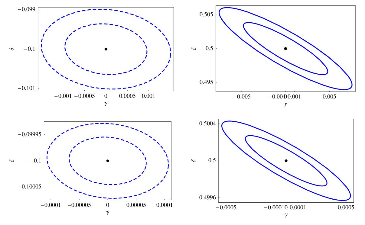
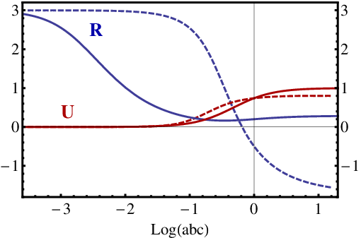
We map our Fisher matrix (8) with the same experimental specifications as in Table 1 into the new parameter space . Our intention is to infer the order of magnitude of the constraints this new cosmological tool would be able to put on the dark energy skewness parameters. We apply the parameter transformation , where . If we assume that the system has just entered the scaling solution, the critical point (14) approximately describes the dependence of the dark energy anisotropy on the skewness parameters at present. In this case we choose for the fiducial model and , namely an ellipsoidal Universe with (see Fig 6) and we choose initial conditions such that . The final attractor value is as expected rather close, . The error contours are shown in the right panels of Fig. 5, for both Gaia and Gaia+ configurations.
Conversely, if the expansion is driven towards a future dark energy dominated solution, equations (13) do not represent the anisotropy parameters at present (see Fig 6). In order to derive a more appropriate functional form for them, we solved the linearized system (12) around solution (13) and we fixed to select the present values. For this second case, results are shown in the left panels of Fig. 5. Notice that Fig 6 depicts a late time expansion history and aims just at illustrating the trend towards the critical points from different values of the anisotropy parameters (namely in an earlier stage, but it might set to be vanishing at decoupling by time dependent skewness parameters in specific models – see [12]).
The constraints on and are in the range . The current limits from SNIa data are then to orders of magnitude weaker [12] and, even if the number of supernovae will substantially increase in the near future, it might be hard to improve the constraints at such a high level because of the integral dependence of the luminosity distance on the skewness parameters. Therefore the cosmic parallax seems to be an ideal candidate for testing the anisotropically stressed dark energy.
The forecastings we presented in this section do not include possible systematic effects. In our Fisher analysis we just took into account the statistical errors. Several spurious effect must be considered by the time real data is available. For instance, the peculiar velocity of the objects need to be considered, although averaging it over a large sample of uncorrelated objects it should be possible to eliminate such a form of bias. Furthermore, this effect decreases with increasing angular diameter distance to the object [24]. The main source of noise however could be due to the aberration change induced by our own motion. Fortunately, both the aberration change and the observer peculiar velocity signal have a dipolar signature whereas cosmic parallax from Bianchi I models results in a superposition of quadrupoles. Other minor effects like the temporal changes of local lensing and microlensing (a parallax disturbances of few nanoarcseconds are expected due to the weak microlensing [29]), were not taken into account, as they require a more detail analysis, beyond the scope of this paper.
V Discussions
Any anisotropy will leave an imprint on the angular distribution of objects that are able to trace cosmic expansion. If such an anisotropy is present before the last scattering surface, the CMB map will also be affected. The temperature field will carry extra anisotropies mainly caused by the angular dependence of the redshift at decoupling. By resolving geodesic equations and expanding temperature anisotropies in spherical harmonics, it is straightforward to relate the low multipole components to the eccentricities of the model [12]. In Bianchi I models the first notable multipoles related to the CMB are the monopole and the quadrupole. The observed value of the latter puts constraints on the shear at last scattering of order , taking into account the cosmic variance. These constraints can be mapped into either magnetic field [9] or anisotropic dark energy limits, depending on the source that gives rise to the anisotropy. In addition, one expects the eccentricities to be non-vanishing if the expansion has been somewhat anisotropic at decoupling. However it is in principle also possible to escape detection from CMB if each scale factor has expanded the same amount since last scattering, no matter how anisotropically. Nonetheless, in all these analysis the anisotropy pattern is directly added to the intrinsic standard FRW perturbations, a simplistic way of treating the signal at large scale. In this still exploratory stage of analysis it is worth stressing that CMB is indeed a very powerful constraint on the shear at the time of decoupling, but with almost no direct impact on late time expansion history. Complementary to that, cosmic parallax, namely the temporal change of angular separation of distant sources, is a direct and potentially powerful test of anisotropy at small redshifts and at present.
The anisotropic stress of dark energy is expected to have a leading role in the generation of anisotropy at late times. It can be parameterized by skewness parameters in the stress-energy tensor formulations, which may be constant or time dependent functions. For example a minimally coupled vector field satisfying quadrupole constraints was presented in [12]. The only way to test these models is to use either the angular dependence of the magnitude or the angular distribution of objects in the sky at recent time, i.e. either distant source angular distribution or the real-time cosmic parallax, the two relying on different techniques and having independent systematics that complement each other.
We adopted a simple phenomenological model to describe late-time expansion of the universe, filled by pressureless matter and an anisotropically stressed dark energy component with two extra degrees of freedom, namely the skewness parameters. No matter what the evolution of both energy densities and shears was at high redshifts, we have shown that Gaia will be able to constrain the skewness parameters up to at 2, comparable to CMB tests at decoupling time, and 23 orders of magnitude better than current supernovae Ia limits [12] (a Gaia+ experiment would improve them by one order of magnitude).
In this paper we discussed in detail the real-time technique; before concluding we comment briefly on the possibility of testing anisotropy through the accumulated effect on distant source (galaxies, quasars, supernovae) distribution.
If sources shifts by as much as 0.1as/year during the dark energy dominated regime, then the accumulated shift will be of the order of 1 arcmin in years and up to fraction of a degree in the time from the beginning of acceleration to now. If the initial distribution is isotropic, this implies that sources in one direction will be denser than in an orthogonal direction by roughly . This anisotropy could be seen as a large-scale feature on the angular correlation function of distant sources, where we expect any intrinsic correlation to be negligible. The Poisson noise become negligible for : for instance, a million quasars could be sufficient to detect the signal. Although the impact of the selection procedure and galactic extinction is uncertain, this back-of-the-envelope calculation shows that the real-time effect could be complemented by standard large-scale angular correlation methods22 2 We are indebted to an anonymous referee for this suggestion..
While finalizing this manuscript another work analysing the cosmic parallax in Bianchi I models came out [25]. Our work differs in many aspects. In [25] the authors focused on the shear in models that isotropize, that is on solutions of the shear dynamical equations that are decreasing function of time. Hence the fact that they find a signal substantially lower than ours is not surprising. In fact, in [25] the background is described by a CDM model where the non-FRW quantities are driven by a constant equation of state. The analysis is restricted to ellipsoidal universes, where the dependence on the azimuthal angle is dropped and the signal is a pure quadrupole. Furthermore in order to accomplish forecasting we have performed a Fisher Matrix analysis of the signal contemplating two different experimental sets, Gaia and Gaia+.
More in general, we have shown that, differently from LTB models with off-centre observers [24], the cosmic parallax signal in Bianchi I models is a combination of two quadrupole functions of the two angular coordinates. Since the most important systematic noises, caused by peculiar velocities and aberration changes, have a dipolar functional form, Bianchi I models seem to be ideally testable, though even in LTB models specific observational strategy aiming at distinguishing the signal from the noise are possible [24].
Assuming that null geodesics are radial, we have provided an analytical expression for the cosmic parallax in general Bianchi I models. This assumption is motivated by a direct numerical calculation of the geodesic for a source at redshift (see Appendix A).
CMB and cosmic parallax detect anisotropy at two different times and, from an observational point of view, are completely independent on each other: combining them together one will have the opportunity to reconstruct the evolution of the anisotropy and test with high accuracy the Copernican Principle.
Acknowledgements
We would like to thank Tomi Koivisto for fruitful discussions.
Appendix A Geodesic equations
Restricting for simplicity to two dimensions, particularly to the (X,Y) plane (where ), we now want to check whether neglecting the curvature of null geodesic equations considerably affects our results. Photons follow trajectories that are described by the ensuing equations:
| (15) | |||||
| (16) | |||||
| (17) |
with the additional constraint (note that here is the redshift, not to be confused with the coordinate Z). Here primes denote derivative with respect to the affine parameter .
In order to solve system (15-17), the scale factors as functions of time are required and hence one has to couple to it the dynamical equations. Since we are integrating backward from the observer position to the source location, typically at redshift of order 1, we need to evaluate these functions in these redshift range. We adopt the linearized solution of the dynamical system (12) in the vicinity of the critical point (13): in this way we take into account the effect of the shear arising from an anisotropically stressed dark energy. The linearized equation for the anisotropy parameters with and are:
| (18) | |||||
| (19) | |||||

The full set of equations with , and is then :
| (20) | |||||
| (21) | |||||
| (22) | |||||
| (23) | |||||
| (24) | |||||
| (25) | |||||
| (26) | |||||
| (27) |
Results for a source located at z=1 are shown in Fig. 7.
References
- [1] A. de Oliveira-Costa, M. Tegmark, M. Zaldarriaga, and A. Hamilton, Phys. Rev. D 69, 063516 (2004), eprint arXiv:astro-ph/0307282.
- [2] P. Vielva, E. Martínez-González, R. B. Barreiro, J. L. Sanz, and L. Cayón, Astrophys. J. 609, 22 (2004), eprint arXiv:astro-ph/0310273.
- [3] M. Cruz, E. Martínez-González, P. Vielva, and L. Cayón, MNRAS 356, 29 (2005), eprint arXiv:astro-ph/0405341.
- [4] H. K. Eriksen, F. K. Hansen, A. J. Banday, K. M. Górski, and P. B. Lilje, Astrophys. J. 605, 14 (2004).
- [5] G. Efstathiou, MNRAS 348, 885 (2004), eprint arXiv:astro-ph/0310207.
- [6] S. Tsujikawa, R. Maartens, and R. Brandenberger, Physics Letters B 574, 141 (2003), eprint arXiv:astro-ph/0308169.
- [7] J. M. Cline, P. Crotty, and J. Lesgourgues, Journal of Cosmology and Astro-Particle Physics 9, 10 (2003), eprint arXiv:astro-ph/0304558.
- [8] S. DeDeo, R. R. Caldwell, and P. J. Steinhardt, Phys. Rev. D 67, 103509 (2003), eprint arXiv:astro-ph/0301284.
- [9] L. Campanelli, P. Cea, and L. Tedesco, Phys. Rev. D 76, 063007 (2007), eprint 0706.3802.
- [10] A. Gruppuso, Phys. Rev. D 76, 083010 (2007), eprint 0705.2536.
- [11] T. Koivisto and D. F. Mota, Journal of Cosmology and Astro-Particle Physics 6, 18 (2008a), eprint 0801.3676.
- [12] T. Koivisto and D. F. Mota, Astrophys. J. 679, 1 (2008b), eprint 0707.0279.
- [13] R. A. Battye and A. Moss, Phys. Rev. D 74, 041301 (2006), eprint arXiv:astro-ph/0602377.
- [14] L. P. Chimento and M. Forte, Phys. Rev. D 73, 063502 (2006), eprint arXiv:astro-ph/0510726.
- [15] A. Cooray, D. E. Holz, and R. Caldwell, ArXiv e-prints (2008), eprint 0812.0376.
- [16] C. B. Collins and S. W. Hawking, MNRAS 162, 307 (1973).
- [17] J. D. Barrow, R. Juszkiewicz, and D. H. Sonoda, MNRAS 213, 917 (1985).
- [18] E. Martinez-Gonzalez and J. L. Sanz, A&A 300, 346 (1995).
- [19] R. Maartens, G. F. R. Ellis, and W. R. Sroeger, A&A 309, L7 (1996), eprint arXiv:astro-ph/9510126.
- [20] E. F. Bunn, P. G. Ferreira, and J. Silk, Physical Review Letters 77, 2883 (1996), eprint arXiv:astro-ph/9605123.
- [21] A. Kogut, G. Hinshaw, and A. J. Banday, Phys. Rev. D 55, 1901 (1997), eprint arXiv:astro-ph/9701090.
- [22] J. D. McEwen, M. P. Hobson, A. N. Lasenby, and D. J. Mortlock, MNRAS 369, 1858 (2006), eprint arXiv:astro-ph/0510349.
- [23] T. R. Jaffe, S. Hervik, A. J. Banday, and K. M. Górski, Astrophys. J. 644, 701 (2006), eprint arXiv:astro-ph/0512433.
- [24] C. Quercellini, M. Quartin, and L. Amendola, Physical Review Letters 102, 151302 (2009), eprint 0809.3675.
- [25] M. Fontanini, M. Trodden, and E. J. West, ArXiv e-prints (2009), eprint 0905.3727.
- [26] F. Ding and R. A. C. Croft, ArXiv e-prints (2009), eprint 0903.3402.
- [27] C. A. L. Bailer-Jones, in IAU Colloq. 196: Transits of Venus: New Views of the Solar System and Galaxy, edited by D. W. Kurtz (2005), pp. 429–443.
- [28] L. Lindegren, C. Babusiaux, C. Bailer-Jones, U. Bastian, A. G. A. Brown, M. Cropper, E. Høg, C. Jordi, D. Katz, F. van Leeuwen, et al., in IAU Symposium (2008), vol. 248 of IAU Symposium, pp. 217–223.
- [29] M. V. Sazhin, V. E. Zharov, and T. A. Kalinina, MNRAS 323, 952 (2001), eprint arXiv:astro-ph/0005418.