Phase diagram of the ABC model on an interval
Abstract
The three species asymmetric model was initially defined on a ring by Evans, Kafri, Koduvely, and Mukamel, and the weakly asymmetric version was later studied by Clincy, Derrida, and Evans. Here the latter model is studied on a one-dimensional lattice of sites with closed (zero flux) boundaries. In this geometry the local particle conserving dynamics satisfies detailed balance with respect to a canonical Gibbs measure with long range asymmetric pair interactions. This generalizes results for the ring case, where detailed balance holds, and in fact the steady state measure is known only for the case of equal densities of the different species: in the latter case the stationary states of the system on a ring and on an interval are the same. We prove that in the limit the scaled density profiles are given by (pieces of) the periodic trajectory of a particle moving in a quartic confining potential. We further prove uniqueness of the profiles, i.e., the existence of a single phase, in all regions of the parameter space (of average densities and temperature) except at low temperature with all densities equal; in this case a continuum of phases, differing by translation, coexist. The results for the equal density case apply also to the system on the ring, and there extend results of Clincy et al.
1 Introduction
One dimensional systems play an important role in statistical mechanics. In addition to their intrinsic interest as models of physical systems in confined quasi-linear geometries, they are in many cases exactly solvable and in fact are, with few exceptions, the only exactly solvable many body systems [1, 2, 3, 4]. These exact solutions provide insights into both equilibrium and non-equilibrium collective behavior in higher dimensions.
An interesting connection between equilibrium and non-equilibrium phase transitions in one dimension is provided by the ABC model introduced by Evans et al. [5] (a model with similar behavior was discussed in [6]): a one dimensional system consisting of three species of particles, labeled , on a ring containing lattice sites (one may equivalently regard it as a model with two species and empty sites, or as a “clock” model with three states). We will here typically let , , or denote a particle type, and make the convention that , , denote the particle types which are successors to in the cyclic order . The system evolves by particle conserving nearest neighbor exchanges with asymmetric rates: (clockwise) with rate , where ; the total numbers of particles of each species are conserved and satisfy . Evans et al. argued that this system will, in the limit with and with for all , segregate into pure , , and regions, with rotationally invariant distribution of the phase boundaries. For the case and , the only case we will consider here, they showed further that when the dynamics satisfies detailed balance with respect to the Gibbs measure of a certain Hamiltonian having a long range pair interaction, so that the stationary state is an equilibrium state.
In a later development Clincy et al. [7] considered a weakly asymmetric version of this model in which ; the stationary state for the equal density case then becomes a Gibbs measure of the form , with energy equal, up to a constant, to the Hamiltonian of [5] divided by . The parameter thus plays the role of an inverse temperature: . (The energy is written as in [7], but here we adopt the convention that quantities with and without a circumflex refer respectively to the ring geometry and to the interval geometry introduced below.) Clincy et al. obtained the Euler-Lagrange equations for the minimizers of the free energy functional, which here is equivalent to the large deviation functional (LDF), of the rescaled particle densities , in the limit with and , and showed that the uniform density profiles are always a solution of these equations, but that for temperatures below the critical temperature there is also a nonuniform solution of the linearized equations which has a lower free energy than the uniform state. They interpreted this as a second order transition at from the uniform to the nonuniform state, and confirmed by numerical simulations that for the system is in a single phase with essentially no correlations (they are ) between the locations of particles of different species, while for there is segregation of the different species. They further argued that this transition will persist (possibly becoming first order) for unequal densities. In this case the stationary state is no longer an equilibrium state and is in fact unknown; despite this, they were able to obtain the LDF to order for all densities (see also [8]).
In the present work we consider the weakly asymmetric ABC system on a one-dimensional lattice of sites with zero flux boundary conditions: the dynamics are the same as above, except that a particle at site (respectively ) can only jump to the right (respectively left). We shall refer to this geometry as an interval. In contrast to the situation on the ring, there is for this system always, whatever the values of , , and , an energy function (see (2.1) below) such that the dynamics satisfies detailed balance with respect to an equilibrium measure .
When the energy for the system on the interval agrees with the energy on the ring [7], in the sense that if we (mentally) connect site to site 1 clockwise, and thus identify each configuration in the interval with a corresponding configuration on the ring, then and agree up to a constant which depends only on the . Thus the probabilities of the configurations and (at the same ) are the same, and the invariance under rotations of implies a rather surprising “rotation” invariance of and of the Gibbs measure on the interval. It follows also that all the results obtained in the present paper for the interval model in the case of equal densities give corresponding results on the ring. When the are not all equal one might of course use similarly to define an energy of a ring configuration, but this energy would then depend on which site is chosen for the origin. The resulting Gibbs measure on the ring would be neither rotationally invariant nor invariant under the time evolution of the ABC dynamics.
Using the Gibbsian nature of the invariant measure and following [7] we can obtain the free energy functional of the density profiles in the scaling limit , . The parameters of the model in this limit are the inverse temperature and the mean densities . Our main goal is to determine, for given values of these parameters, whether has a unique minimizing profile or whether, conversely, there is more than one minimizer and thus coexistence of phases, and in either case the form of the minimizing profile(s). We are able to establish uniqueness at high temperatures by a direct study of the functional . We further show that minimizers must satisfy the Euler-Lagrange equations for , and by a study of the solutions of these equations we establish the nonuniqueness of minimizers when and ; the nonuniqueness corresponds to the lack of rotational invariance for the minimizers on the ring. Conversely, we establish uniqueness of the minimizers (on the interval) whenever the densities are not all equal. In the process we also obtain the form of the minimizing density profiles as elliptic functions corresponding to pieces of the periodic trajectory of a particle moving in a quartic confining potential.
We remark that work on the ABC model on the ring has been carried out recently by Bodineau et al. [8]. They investigated analytically the pair correlations, and thus also the local density fluctuations, in the uniform state, and showed that the latter diverge as . They also suggested a possible formula for the large deviation and discussed the possibility of deriving this from the macroscopic fluctuation theory [9]. The model on the ring was also studied, in a different context, by Fayolle and Furtlehner [10], who obtained results which agree, for the case in which the system on the ring has the same stationary Gibbs measure as does the system on the interval, with those obtained here. Results concerning the relation between the hydrodynamic equations for the ABC model and the LDF were obtained by Bertini et al. [9].
The outline of the rest of the paper is as follows. In Section 2 we define the Gibbs measure with respect to which the dynamics satisfy detailed balance. We then study some properties of this measure; in particular, we describe its ground states, which are nonunique whenever two species have equal mean densities which are greater than or equal to . We investigate also some properties of the microscopic correlation functions at finite-temperature: the mean field nature of the interactions in this system leads in the limit to local measures which are exchangeable.
In Section 3 we consider the scaling limit of the model and briefly discuss the nature of possible limiting density profiles. In Section 4 we obtain the Helmholtz free energy as a functional of the scaled densities (this is equivalent to obtaining the LDF) as well as the Euler-Lagrange equations satisfied by minimizers of ; the proof that minimizers exist and must satisfy these equations is postponed until Section 10. In Section 5 we investigate the minimizers of by studying in detail the solutions of the Euler-Lagrange equations. These solutions, which describe all stationary points of , are given by periodic (elliptic) functions describing the motion of a particle in a one dimensional quartic potential. There are many such solutions for large ; despite this, we prove uniqueness of the globally minimizing density profiles for all so long as the mean densities are not all equal. Details of the uniqueness proof are given in Sections 6 and 7. In Section 8 we discuss the phase diagram of the model and describe a perturbation expansion around the uniform state. In Section 9 we show that is a convex functional of the ’s (with fixed ’s) at high temperature, which gives an alternate proof of the uniqueness of minimizers of in this regime. A concluding discussion is given in Section 11.
2 The steady state of the model
A configuration of the ABC model on the interval is an -tuple , with , , or . We will let be a random variable which specifies whether a particle of species is present at site : if and otherwise, so that and . The time invariant measure for the weakly asymmetric dynamics described in Section 1 is a canonical Gibbs measure,
| (2.1) |
where
| (2.2) |
and is the usual equilibrium normalization factor, that is, the (canonical) partition function with fixed particle numbers . To verify this invariance one checks detailed balance for the dynamics: if is a configuration with particles of types and on sites and , respectively (recall the convention that , , …run cyclically through , , and ), and is the configuration with these particles interchanged, then the transition rates are that at rate and at rate , and the detailed balance condition follows from (2.1) and (2.2). For , is the unique stationary measure; this follows from the transitivity of the dynamics on the set of all configurations consistent with . When all these configurations are equally likely.
One can rewrite (2.2) in various forms which differ from each other only by functions of , , and , and this does not affect when the are fixed. As an example, an equivalent energy is
| (2.3) |
We shall generally use the form given in (2.2), as it clearly exhibits the cyclic symmetry between the different species.
Remark 2.1.
(a) The energy of (2.3) is of particular interest when the species is not present, i.e., when . In this case we may call the particles just particles and the particles holes, and the model reduces to the weakly asymmetric simple exclusion process (WASEP). Then , which is the energy arising from an external field of magnitude pushing the particles to the right. See [11] and Section 7.2.2 of the review [12] for discussions of the partially asymmetric simple exclusion process on an interval.
(b) On the ring, the stationary measure for the WASEP gives equal weight to all configurations. In contrast to the situation on the interval, however, the dynamics is not reversible, i.e., does not satisfy detailed balance, with respect to this stationary measure. We thus have a true nonequilibrium stationary state (NESS).
2.1 Ground states
For there are many configurations stationary for the dynamics: all those of the form , where a boldface letter denotes a block of particles of the corresponding species. These configurations are local minimizers of the energy , in the sense that any interchange of adjacent particles of different species will raise the energy, but not all of them are obtained as limits of when . In this limit the measure will be concentrated on the ground states of , that is, on the global minimizers of [13]. As we will see, the energy per particle in the ground state is , where .
We describe the ground states by considering several cases. It is helpful to note that (2.2) may be summarized as saying that there is a contribution of to the energy each time a particle lies to the left of an particle, a to the left of a , or an to the left of a . We also remark that if a local minimizer contains a sequence of four blocks with a total of particles of type , then one may lower the energy by regrouping these particles into three blocks, , , or , unless (and similarly for and ).
(i) If one species is not present, say , then the ground state energy is zero and there is a unique ground state configuration with all particles of type to the left of all particles of type . This is the WASEP discussed in Remark 2.1. In this case there are no local minimizers other than the global minimizer.
From now on we suppose that none of the vanish.
(ii) If one of the is greater than the other two, say (other cases can then be found by cyclic permutation), then it is easy to see that there is a unique ground state consisting of three blocks ordered as , with .
(iii) If two of the are equal and the third is smaller, say , the ground state will be fold degenerate, consisting of three or four blocks ordered as , , or , that is, some of ’s will be at the left side of the interval, followed by all the ’s, then all the ’s, and finally the remaining ’s. Here .
(iv) If all of the are equal, , then the ground states are the shifts, by an arbitrary number of sites, of the configuration with three blocks ordered as ; see the discussion in Section 1 of the correspondence in this case with the model on the ring. The ground state is thus -fold degenerate, and .
The ground state phase diagram of the system in the right triangle where and is given in Figure 1 (remember that ). The ground state is unique everywhere except on the three line segments originating from and terminating at the midpoints of the sides of the triangle, corresponding to cases (iii) and (iv) above. On the edges of the triangle the system reduces to the WASEP.

2.2 Finite temperature correlations and local states
The correlation functions at finite are
| (2.4) |
where denotes the expectation with respect to the Gibbs measure . We point out here some simple relations that these satisfy, both in finite volume and in the limit , . (With some abuse of notation we will use to denote both the density in a finite system and the limiting value of the density in the limit.)
First, it is easy to check from (2.1) and (2.2) that, whenever all the are positive,
| (2.5) |
and this implies that for all ,
| (2.6) |
Note that when and the system on the interval coincides with that on the ring, (2.6) is a consequence of the translation invariance of the latter.
Next we note that there is a constant , which depends only on and the , such that for fixed , and integers with , and , , and distinct particle species,
| (2.7) |
where denotes the largest integer less or equal to . To see that the limit in (2.7) is independent of , , , , , and we first write , , and , and observe that if is a configuration with , , and , and is the configuration on sites which is obtained from by omitting the sites , , and and renumbering, then ; here the terms arise from those terms in the energy (2.2) involving the particles on sites , , and , and , which depends on , the , and the , satisfies . Thus from (2.1) and (2.2),
| (2.8) |
The corresponding expression for a different choice of the and will differ from (2.8) only in the replacement of by some , from which the result follows.
The results (2.6) and (2.7) are closely related: each shows that a product of three occupation numbers, or their expectations, is site independent. We will see another such relation in Section 5: for all scaled density profiles which are stationary points of the free energy functional (see Section 4) the product is in fact independent of .
Similar identities can help us understand the nature of local states [14] in this model. By the local state at position we mean the infinite volume state, if it exists, whose correlation functions for particles of type at sites are given by
| (2.9) |
(If such a local state does not exist then one may identify subsequences along which all the limits (2.9) do exist, and thus obtain a family of local states.) An argument similar to that establishing (2.7) shows that for , fixed, and any permutation of ,
| (2.10) |
This implies [15] that is a product measure or a superposition of product measures, which of course reflects the mean field nature of the interaction. Dynamically this corresponds to the fact that when , the exchanges become symmetric and the invariant measures are just superpositions of extremal product measures [14]. (In fact this last argument applies also on the ring with unequal densities .)
3 The scaling limit
We now turn to the properties of the model in the macroscopic scaling limit
| (3.1) |
We say that there is a unique (macroscopic) density profile in this limit when there exists a function such that [16]
| (3.2) |
for all , all , and all piecewise smooth functions on the interval [0,1]. Such must, of course, satisfy the conditions
| (3.3) |
Equation (3.2) expresses the convergence, in a certain sense, of the random profile to the non-random profile : specifically, for each the random variable converges in the sense of (3.2) to the non-random quantity . It may happen, on the other hand, that the limiting profile is itself random, in the sense that there is some family of limiting profiles , indexed by the variable lying in some sample space and each satisfying (3.3), and a measure on , such that for each test function ,
| (3.4) |
in the sense of convergence in distribution. (In fact, (3.2) is also convergence in distribution, to a non-random limit.) We would then say that the limiting profile is not unique and that the system can exist in more than one phase, i.e., is in a phase transition region. This is exactly what happens to the ferromagnetic Ising model in two or more dimensions in a periodic box at temperatures below the critical temperatures and fixed magnetization , where is the spontaneous magnetization [17]. In our system this happens, as we shall see, if and only if and . More generally, it may be that the limit in (3.4) will not exist; in that case, one would expect to obtain a limit in the given form by passing to a subsequence.
4 The free energy
The question of whether or not there exists a limiting profile(s) as given by (3.2) or (3.4), and of which of these alternatives applies, is related to the question of the existence and uniqueness of minimizers of the LDF for this system [18]. If denotes a general continuum density profile satisfying (3.3) (written in terms of rather than ) then the logarithm of the probability of finding the profile in the scaling limit is asymptotically , where is the LDF. Possible limiting density profiles are thus those which minimize .
To obtain from the microscopic measure the probability of finding the profile it is necessary (roughly speaking) to sum , as given in (2.1), over all (microscopic) configurations consistent with ; this summation will yield a restricted partition function divided by the full partition function . Taking the logarithm of this ratio, dividing by , and taking the scaling limit of the result will then yield
| (4.1) |
where is the Helmholtz free energy of the system restricted to having a density profile :
| (4.2) |
Here the macroscopic energy and entropy are the limits of the microscopic energy and entropy per site; as indicated, these limits depend only on the profile . For the energy, this is due to the mean field nature of the microscopic energy of (2.2). For the entropy, which is the logarithm of the number of microscopic configurations consistent with , this is due to the Bernoulli nature of each component of the local measure, which implies that all microscopic configurations consistent with have the same energy and hence the same weight. Thus
| (4.4) | |||||
| (4.5) |
The profiles minimizing (4.5)—that is, the candidates for limiting density profiles—will represent a compromise between the entropy, which wants to keep all the densities uniform, and the energy, which wants to keep the different particle types segregated.
The next theorem establishes the existence and properties of these minimizers.
Theorem 4.1.
Suppose that . Then given positive numbers , , and with , let denote the infimum the values of over (measurable) profiles satisfying the constraints (3.3). Then there exist infinitely differentiable functions , and , possibly non-unique, that satisfy these constraints and achieve the minimum:
| (4.6) |
Moreover, there is a so that each satisfies for all ; thus the minimizer is an interior point with respect to the constraint of taking values in and so satisfies the Euler-Lagrange equations (ELE) obtained from .
The proof of this theorem is given in Section 10. We note here, however, that the minimizers lie in the interior of the constraint region essentially because the entropy term has infinite normal derivative at the boundary. For , when only the energy counts, the densities minimizing will be the continuum limit of the ground state configurations described in section 2.1 and need not satisfy the ELE.
To obtain the Euler-Lagrange equations satisfied by the minimizing profiles we must take the variational derivatives of with respect to two of the density profiles while maintaining and ; here we will treat and as independent, with . Defining to be the variational derivative taken as if the profiles , , and were independent, we will then have
| (4.7) |
Imposing the constraints leads to the ELE
| (4.8) |
where
| (4.9) |
Simple manipulations then show that under the constraint the derivatives satisfy
| (4.10) |
which implies, rather surprisingly, that solutions of (4.8) will satisfy for all , i.e., that the functional derivatives of can be taken as if the were independent. From (4.9), then, the minimizing profile must satisfy the ELE
| (4.11) |
for all . It follows that
| (4.12) |
which is consistent with (2.5). The ELE may also be written in differential form:
| (4.13a) | ||||
| (4.13b) | ||||
| (4.13c) | ||||
These equations were derived in [7] for the case . One obtains minimizing profiles by solving these equations with the constraints
| (4.14) |
Remark 4.2.
As indicated above, one may consider as a function of and alone, with . The corresponding variational derivatives and are the local chemical potentials for the density profiles,
| (4.15) |
which are constant at a stationary point of (see (4.8)). These are given by
| (4.16) | |||||
| (4.17) | |||||
with the replacements and .
5 Solutions of the ELE equations
We now turn to a detailed study of the solutions of the Euler-Lagrange equations (4.13) with the constraints (4.14). As already noted in Theorem 4.1, for any given and there must exist at least one solution of these, corresponding to a minimizer of . There may, however, be many solutions; these will all correspond to stationary points of , and more than one of these stationary points may be a minimizer. In this section we determine all the minimizers.
5.1 The WASEP
We first consider briefly the case in which one of the densities is zero, say , when the system reduces to the WASEP (see Remark 2.1). This system, which can be solved explicitly on the interval, has in the scaling limit a unique limiting density profile—i.e., minimizer of the free energy—given by the solution of (4.13) with :
| (5.1) |
The constant is determined by the constraint . When , (5.1) reduces to the ground state configuration in which all the particles are pushed to the right:
| (5.2) |
The local measure in this model is, as expected, the Bernoulli measure with density . (On the ring the stationary state of the WASEP is a nonequilibrium one in which all configurations have equal weight and the limiting scaled density profile is constant.)
5.2 Properties of solutions.
Through the remainder of this section we suppose that all the are strictly positive. Let us begin by discussing the properties of some given solution of the ELE equations (4.13) with the constraints (4.14). By differentiating with respect to we see that the ELE imply that there is a constant such that
| (5.3) |
and that the condition
| (5.4) |
is preserved by the equations. Equation (5.3) is the scaling limit version of (2.7).
Since and have sum and product they must be the two roots of the equation , from which
| (5.5) |
Then squaring (4.13b) and using (5.5) we find that is a solution of
| (5.6) |
where
| (5.7) |
Of course, the same argument shows that and must also be solutions of (5.6).
To study (5.6) we write and let ; then satisfies
| (5.8) |
This is the equation of the zero energy solution of a mass 1 particle moving in a potential . Because is quartic in the solutions are elliptic functions; see Appendix A. For , is strictly positive for and so no solutions with in this range exist. For , has a local minimum with value 0 at , and (5.8) has constant solution . For , has four zeros, , , , and , where and for . See Figure 2. Since we are interested in solutions of (4.13) which satisfy we consider only the solutions of (5.8) which oscillate between and . Let denote the solution of (5.8) which satisfies ; then has period
| (5.9) |
For , is determined by inverting the relation
| (5.10) |
is then obtained for all by extending to an even function of period .

Remark 5.1.
We note some properties of this solution; those listed in (a) are elementary, and we relegate the proofs of (b) and (c) to Appendix B.
(a) is even, is periodic with minimal period , has local minima at integer multiples of and local maxima at half integer multiples of , and is monotonic between these points. Moreover, if and only if either or is an integer multiple of .
(b) and . Moreover, for any ,
| (5.11) |
and
| (5.12) |
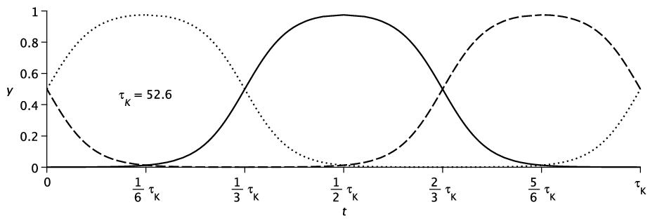
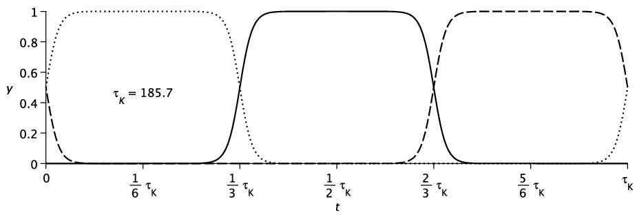
This means that in the limit the trajectory will spend two-thirds of its time near the origin and one-third near ; see for example the third trajectory shown in Figure 4.
(c) is a strictly monotonic decreasing function of for .
Now for there must be a phase shift such that
| (5.13) |
that is, each is obtained by looking at the solution within a window of length centered at some value , and rescaling from to . The phase shifts are not independent; in fact,
| (5.14) |
(see (27) of [7]). In verifying (5.14) the requirement (4.14) of certain average densities is not relevant. What matters is that we consider three solutions of the ELE (4.13) or equivalently (with the rescaling ) three solutions of (5.8) satisfying
| (5.15) |
with . We may assume that these are defined for all and without loss of generality that . It is helpful to view the trajectories in the - phase plane; see Figure 3. At time the B trajectory lies at the point on the axis marked B1. Since the velocity on the B trajectory is zero at this point, it follows from (5.15) that , that is, the A and C trajectories lie at points such as those marked A1 and C1, respectively; again from (5.15) we know that A1 must be in the upper half of the phase plane, since . Now follow the motion for a time period until reaches the axis at point A2; since now it follows that the B and C trajectories are at points B2 and C2 with equal coordinates, and it follows immediately (using the symmetry around the axis) that the travel time along each of the six orbital segments in the figure is . Thus , , and .

Let us introduce the notation
| (5.16) |
where , for the average of the function over the set (which will always be a union of intervals), and define . Then with (5.13) and (5.14), (4.14) becomes
| (5.17) |
The problem of solving (4.13) and (4.14) is now the problem of finding and satisfying (5.17). If either so that is constant, or is an integer multiple of , then is constant and (5.17) has a solution (with arbitrary ) if and only if .
Figure 4 shows the curves and for several values of . To obtain a solution of (5.17) for some one views the corresponding three curves in a window of length (corresponding to the full lattice, i.e., to the original unit interval after the variable change in (5.13)) centered at . In this context we label a solution by an integer which is one more than the number of full periods (plus, perhaps, a fraction of a period) fit into the window: we say that a solution of (5.17) with is of type , for , if
| (5.18) |
We do not assign a type to the constant solution , which exists for , , and every value of , as discussed above.

5.3 Uniqueness of solutions
The next theorem summarizes our results about solutions of the ELE and answers the questions posed in the first paragraph of this section. We consider the problem of finding and satisfying (5.17).
Theorem 5.2.
(a) If then there exist (i) the constant solution, (ii) for , , a solution of type unique up to translation, and (iii) no other solutions. The minimizer of the free energy is, for , the (unique) constant solution and, for , the type 1 solution.
(b) For values of other than there exists for all a unique type 1 solution which is a minimizer of the free energy.
In the remainder of this section we prove part (a) of this theorem and give an overview of some parts of the proof of part (b). More technical parts of the proof of (b) are given in Sections 6 and 7. Before beginning, we summarize some simple properties of the function of (5.17).
Remark 5.3.
(a) As remarked above, if either or is a multiple of then for all .
(b) For all other than those of (a) a plot and will look much like one of the sets of curves in Figure 4. In particular, since is even and -periodic, so is , and from it follows that is strictly monotonic between integer multiples of . From this we see that if then either or must be an integer multiple of .
(c) To find all triples for which (5.17) has a solution for a given it suffices to consider values of satisfying . For such the possible triples satisfy ; other orderings of the same sets of values are found for other ranges of .
Proof of Theorem 5.2(a): When , (5.17) becomes
| (5.19) |
For every , one solution of (5.19) is the constant corresponding to . Moreover, if then by Remark 5.1 there exist one-parameter families of nonconstant solutions (indexed by ) obtained by solving
| (5.20) |
for . Note that the solution (5.20) is of type . No other solutions are possible, because (5.19) is inconsistent with the final observation in Remark 5.3(b).
To complete the proof we note that, as is easily seen, perturbing the uniform solution via , where and , decreases the free energy when , so that this solution cannot be a minimizer, and that we will prove in Section 7 (see Theorem 7.1) that no solution of type with can minimize the free energy. ∎
Proof of Theorem 5.2(b): It was shown in Theorem 4.1 that for any positive , , and which satisfy there exists at least one minimizer of the free energy , and that this minimizer satisfies the ELE. By Theorem 7.1 no solution of type with can minimize the free energy, so this minimizer must be of type 1. It remains to prove uniqueness of this solution; we will give the full proof in Section 6 (see Theorem 6.1), but here we illustrate the idea of the proof by sketching the argument for the special case , , in which symmetry considerations considerably simplify the discussion.
We suppose then that for some such and some there are two distinct type 1 solutions of (5.17), and derive a contradiction. It follows from and Remark 5.3(b) that the phase shift must be zero for each solution, so that we are looking at some and on the interval which satisfy (see (5.16))
| (5.21) |
We take and write , so that (because these are type 1 solutions) . The situation is as in Figure 5;

the qualitative features of this figure, which we use below, are obtained from (which holds because , the smallest positive zero of the potential (5.7), decreases with ), the symmetry, and the fact that (5.21) implies that the curves and must cross in the interval . In the full proof below we will verify that the curves cross exactly twice, as shown.
We write and and observe that
| (5.22) |
Since is a (weighted) average of and , necessarily
| (5.23) |
Moreover,
| (5.24) |
where the first inequality holds because is decreasing to the left of the origin and increasing to the right, and the second because on . But then
| (5.25) | |||||
which contradicts (5.22). ∎
6 Uniqueness of type 1 solutions
Our goal in this section is to prove
Theorem 6.1.
Throughout the section we will consider two solutions of (5.8) with ; we write rather than , , for the corresponding periods, and note that by Remark 5.1(c). We begin with a preliminary result.
Lemma 6.2.
(a) For any and the curves and intersect exactly once in the interval .
(b) (i) If then
| (6.1) |
and (ii) if in addition then
| (6.2) |
Proof.
(a) Suppose that is even so that is increasing on the interval ; the proof for odd is similar. For all and the zeros and of (see (5.7)) satisfy
| (6.3) |
and since and , the existence of at least one intersection follows from the intermediate value theorem. On the other hand, if for some then from (5.7) and (5.8), , and this is inconsistent with the existence of two such intersection points.
(b) It follows from (a) that for any , and can intersect at most once on any interval of monotonicity of ). Thus it suffices to verify that (6.1) and (6.2) hold for and . For (6.1) this follows from (see (6.3)) and
| (6.4) |
For (6.2) it follows from and
| (6.5) |
where at the last step we have used monotonicity of on and the condition . ∎
In the remainder of this section we suppose that, given appropriate phase shifts, the solutions and considered above provide two type 1 solutions satisfying (5.17)–(5.14) for the given , , and , and from this derive a contradiction. It is convenient to view these solutions in the same interval, which we take to be . This means that there are phase shifts and such that if and for , then
| (6.6) |
By Remark 5.3(c) we may again assume that and that
| (6.7) |
The fact that these are type 1 solutions, and our assumption that , imply that
| (6.8) |
The key idea in the proof is the same as that for the simple case considered in Section 5.3, but the general case presents two additional difficulties. First, without guidance from symmetry the choice of the intervals and is more delicate, and in fact we must consider two distinct cases in which they are chosen by different prescriptions. Second, one must in some cases apply the reasoning to and , and in others to and , and one must show that one or the other is possible. Sorting out these cases requires some detailed analysis of the geometry of the curves.
Proof of Theorem 6.1: Equation (6.6) implies that the curves and must intersect at least once in the interior of the interval , and since the length of is less than , Lemma 6.2(a) implies that they cannot intersect more than three times. On the other hand, from (4.12) it follows that . It is convenient then to consider two possible alternatives:
z1: , , and the curves and intersect precisely twice within ;
z2: , , and either both inequalities are strict and the curves intersect precisely twice within , or both are equalities and the curves have one intersection within .
A similar analysis leads to corresponding alternatives for and :
w1: , , and the curves and intersect precisely twice within ;
w2: , , and either both inequalities are strict and the curves intersect precisely twice within , or both are equalities and the curves have one intersection within .
We will first show that if z1 (respectively w1) occurs then the argument of Section 5.3 may be applied to and (respectively and ) to derive a contradiction. Then we show that either z1 or w1 or must occur.
Now observe that necessarily . For otherwise, , so that is increasing on and by Lemma 6.2(a) cannot intersect more than once there. It is then helpful to further subdivide the situation into two cases in which we can explicitly identify intervals on which is monotonic:
Case 1: . In this case we write , where , , and .
Case 2: . Here we write , where and .
Then is decreasing on and and increasing on .
Suppose now that z1 occurs. Since and it follows from Lemma 6.2(a) that and intersect once on . We now consider separately the two cases introduced above.
Case 1: Define and , so that . Since has length , we again have (5.22) and therefore (5.23). Moreover, (5.24) follows from the monotonicity of on and then the fact that on , which follows from this monotonicity, Lemma 6.2(a), and the fact that intersects on . But then we may deduce a contradiction between (6.6) and (5.22), just as we did in (5.25).
Case 2: The argument is similar. Let , where and . Let , where and , be an interval of length satisfying , with and chosen so that
| (6.9) |
Now by arguing as in Case 1 we find that (5.24) holds with and replaced either by and or by and . Averaging these two equations (the weights for this averaging,
| (6.10) |
are independent of by (6.9)) we again find that (5.24) itself holds, and the argument proceeds to a contradiction as in Case 1.
If w1 occurs then we may derive a contradiction similarly: we need only replace by throughout and change the sign of some of the inequalities.
It remains to show that either z1 or w1 must occur; to do so we assume that z2 occurs and show that then w1 must also. The occurrence of z2 implies that we must be in Case 1, i.e., that
| (6.11) |
since if there can be no intersection of and on and hence the two intersections of these curves must occur on and , while if then there are three intersections which must occur on , and . We claim further that necessarily
| (6.12) |
For if (6.12) does not hold then
| (6.13) |
Here for the first inequality we have used (6.7), (6.8), (6.11), and the falsity of (6.12), which together imply that
| (6.14) |
and then the monotonicity of on . For the second inequality we use Lemma 6.2(b.i), which is applicable by (6.14). But now
| (6.15) | |||||
which implies w1. Here the first inequality is from Lemma 6.2(b.ii), applicable because (6.7), (6.8), and (6.11) imply
| (6.16) |
and (6.11) implies that and so , and the second from (6.12) and the monotonicity of on , which is applicable by (6.16) and the observation that (6.11) implies that . ∎
7 Solutions of type ,
It is easy to see that type solutions of (5.17) with do exist for certain but not all values of and . The next result, however, shows that these solutions are not of physical interest.
Theorem 7.1.
No type solution of (5.17) with minimizes the free energy.
We begin by rewriting the free energy in terms of the variable . Consider then triples of functions, defined in some interval of length and satisfying and . The free energy of is (see (4.5))
| (7.1) |
where
| (7.2) |
is the energy and
| (7.3) |
the entropy. We will use a rearrangement procedure for these triples.
Let be a partition of and for let . Given a permutation of we may rearrange the intervals in , together with the restrictions of to each interval, into the order , thus defining in the obvious way a new function on , the rearrangement of . A formal definition of (which we will not use in the sequel) may be given as follows: The permuted intervals arise from the partition , with , and this permutation is implemented by the map defined by
| (7.4) |
The rearrangement of is then , i.e., .
The entropy of and are the same. The energy of is
| (7.5) |
where
| (7.6) |
and for , with ,
| (7.7) | |||||
It is natural to think of (7.7) as expressing as a sum of “self energies” of the restrictions of to the intervals and “interaction energies” between the portions of in different intervals. The energy is obtained similarly; the self energy contribution will be the same and the interaction energies will differ only for interval pairs whose order is interchanged by the rearrangement; thus
| (7.8) | |||||
where
| (7.9) |
Proof of Theorem 7.1: Suppose that the triple as above gives a solution of (5.17) on the interval ; specifically, this means that for some and some phase shift , , , and , , and . Suppose also that the solution is of type for some , which implies in particular that . We will show that for some rearrangement of the change in free energy (7.8) is negative. Since clearly for all , will satisfy the same constraints as ; thus cannot be a minimizer of the free energy under those constraints.
The desired rearrangement will be defined in terms of a partition with , for , and ; here is the largest integer such that and is the smallest integer such that . Note that here and have length at most and , , has length exactly . It is easy to see that , so that from (5.18), and in particular .
Now for each , , there will be an such that for all (see Figure 4); we will then say that is a full -interval if it has length and a partial -interval if it has length less than (which is possible only if or ). The types of the intervals are in cyclic order (again see Figure 4): if is an -interval then is an -interval. Recalling that we focus on four consecutive intervals . Without loss of generality we may assume that is an -interval, and we will then write , , , and , i.e., the initial configuration is . Consider then the permutation of these intervals in which we first exchange and , then interchange with (they are now adjacent) and with , and finally exchange and , leading to . We will show that this rearrangement lowers the energy, completing the proof of the theorem.
The calculation is simplest when all four of the intervals are full, so we consider that special case first. For a full -interval we have and , where
| (7.10) |
and so . We may then compute from (7.9) and (7.10) the energy difference arising from reversing the order of a full -interval and a full -interval , where : if then , while if then , where . Rearranging the intervals as above thus first increases the energy by , then decreases it by ; the final exchange of and leaves the energy unchanged. The net change of energy is .
We now consider the general case in which either or or both may be partial intervals. After a translation, if necessary, of by a multiple of we may assume that , , , and for some with ; the condition comes from the fact that if is full then and if is full then , while if both are partial then . The energy change from the rearrangement is the sum, with , of
- •
from the exchange of and ,
- •
from the exchange of and ,
- •
from the exchange of and , and
- •
from the exchange of and .
This energy may conveniently be expressed in terms of
| (7.11) |
using
| (7.12) |
and
| (7.13) |
(see Figure 6). Finally, if we introduce the strictly positive quantities and , then the total energy change may be written, using the identity displayed in (7.13), in the manifestly negative form
| (7.14) |
∎

Remark 7.2.
Energy considerations for full intervals correspond closely to those of single particles: cyclic order is energetically favored, the energy cost of a reversed pair , , or is independent of the species involved, etc. The conclusion above that is favored over parallels the conclusion of Section 2.1 that the ground state of a particle system with a majority of ’s has a block containing all the between blocks of the ’s and the ’s. For partial intervals, energy considerations are more subtle; the final step in the rearrangement above, the interchange of and , is irrelevant when these intervals are full but is needed when they are partial because is richer in species than in and the reverse is true for .
8 Phase diagram of the ABC model
Our results about the minimizers of for specified , , and provide the following picture of the canonical phase diagram of the model (see Fig. 7). The three first order lines in the plane, discussed in Section 2, do not extend to finite temperatures. There is a first order line for which starts at and terminates at the critical temperature , i.e., as one crosses this line by varying the overall densities , the density profiles change discontinuously for . On the line of equal densities the transition at is second order; the divergence of the variance in local density fluctuations as one approaches from above on this line was investigated by Bodineau et al. [8] via a study of the dependence of the correlation function.

To see how the density profiles change as a function of the average densities near the line we take and vary . The density profiles change continuously at high temperatures as the profiles become uniform at . However, when , the particles prefer to be in the middle section of the interval for and to be symmetrically arranged at both ends for , and this change of profile is discontinuous. To see this discontinuity we define an order parameter,
| (8.1) |
and calculate it in the steady state. Figure 8, shows the order parameter as a function of for and . Clearly, for low temperatures, , shows a discontinuity at density .

8.1 Perturbation expansion
In this section we apply a perturbation expansion to calculate the density profiles for average densities which deviate slightly from . In particular we carry out a perturbation expansion of the profiles for average densities , and with small parameters and . For the density profiles are homogeneous (namely, ) at high temperatures, and they become non-homogeneous at . We now expand the density profiles around the homogeneous densities:
| (8.2) |
with small deviations and which satisfy . As a result of this constraint, one is left with two independent functions which we choose to be and . The average densities are then fixed by,
| (8.3) |
where, for convenience, the interval is taken to be . In terms of and the equations for the minimizers (4.13) reduce to
| (8.4) | |||||
| (8.5) |
We proceed by expanding and in terms of two small parameters and , which, at the end of the calculation, will be determined by and . To be explicit, let us write
| (8.6) |
where and are functions of which are of order in the small parameters and . To first order in and (8.5) yields the following equations for and
Solving these equations one finds
| (8.7) | |||||
| (8.8) |
with . Expanding and to second order in and the following equations are obtained for and ,
| (8.9) | |||||
| (8.10) |
These equations can be solved to yield
| (8.11) | |||||
| (8.12) |
The equations for the third order terms, and , are then
| (8.13) | |||||
| (8.14) |
where . To proceed with the analysis one eliminates from the equation for to obtain the following second order differential equation for
| (8.15) |
This equation may be solved to yield
| (8.16) |
Inserting this solution in (8.13) results in the following solution for
| (8.17) |
In summary, to third order in the density profiles are given by
| (8.19) | |||||
| (8.21) | |||||
| (8.22) |
To third order in these equations may be reexpressed as
| (8.23) | |||||
| (8.24) | |||||
| (8.25) | |||||
| (8.26) |
with
| (8.27) |
The expansion parameters and may be expressed in terms of and using (8.3). This leads to
| (8.28) | |||||
| (8.30) |
For a nonzero solution of (8.30) exists only if , and thus by (8.27) only if , i.e., . For , then, all profiles are homogeneous. For there exist type solutions with and small whenever is just above . Their amplitude is determined by via (8.27) but and are otherwise undetermined, corresponding to the translation invariance of the set of solutions.
For non-vanishing or it is convenient to expand (8.30) to third order:
| (8.31) | |||||
| (8.33) | |||||
| (8.35) | |||||
| (8.37) |
Then (8.37) has one or more non-vanishing solutions for or at any temperature. The equilibrium (minimizing) solution is the one which is of type . The minimizing density profiles, as has been shown, are non-homogeneous both above and below ; they vary continuously with the temperature , and no phase transition takes place.
The small and expansion may be used to verify the first order nature of the transition at just below the critical point. To demonstrate this point we take, for simplicity, and consider small and with . In this case , the amplitude satisfies
| (8.38) |
and the density profile is given by
| (8.39) |
At , equation (8.38) has three solutions,
| (8.40) |
Since the stable solution satisfies , it follows from (8.38) that for the stable solution one has . Thus for the negative solution is stable and , while for the positive solution is stable and . The density profile is therefore discontinuous at ; see Figure 8.
9 Convexity of the free energy at high temperature
It follows from Theorem 5.2 that if then for any positive , and with there is a unique solution of the ELE (4.13) with the constraints (4.14); that is, a unique stationary point of the free energy under those constraints. One would then like to know also the nature of the fluctuations about this equilibrium profile, and in particular to show that these fluctuations are Gaussian with a finite covariance. To establish this it is necessary to show that the free energy has a positive definite second variation at the minimizer in the space of density profiles satisfying the above constraints, which implies that it is a strictly convex functional in a neighborhood of the minimizer. We believe that this is indeed true generally, with the obvious exception of the line segment , . In this section we show a global convexity property in a restricted temperature range: for , (with the mean density of species constrained to be ) is globally strictly convex.
To establish the convexity we compute the second variation. Consider the free energy functional on the convex set of nonnegative densities satisfying
| (9.1) |
To make the variations, let and be bounded continuous functions with
| (9.2) |
Then for small values of ,
| (9.3) |
is an admissible variation, and all admissible variations are of this form.
The order contribution from the entropy is
| (9.4) |
where we have used the fact that for any positive , , and with the matrix
| (9.5) |
is positive semidefinite, since its diagonal entries are nonnegative and its determinant is . Because the energy is quadratic, the order contribution from the energy is independent of ; it is
| (9.6) |
However, since for functions and with ,
| (9.7) |
(9.6) reduces to
| (9.8) |
Now let be the Hilbert space of square integrable functions on with , and define on operator on
| (9.9) |
where is the orthogonal projection onto in . Then it is easy to see that
| (9.10) |
Combining the entropy bound (9.4) with (9.8) and (9.10), we see that the second variation is bounded below by
| (9.11) |
We need to show that this quadratic form is nonnegative definite for , which we shall do with a spectral calculation.
To do the calculation, define
| (9.12) |
Then one has
| (9.13) |
If we now write
| (9.14) |
then (9.11) becomes
| (9.15) |
This is nonnegative as long as , which proves the strict positivity of the second variation, and hence the convexity of for such
We also remark that if in the equal density case one considers quadratic variations around the constant profile then one can improve the lower bound (9.4) on the second variation of the entropy to
| (9.16) |
Some modification of the remainder of the argument then shows that the constant profile is indeed a local minimum all the way to .
10 Existence of minimizers
In this section we prove Theorem 4.1, that is, we show that there exist profiles which minimize the free energy functional of (4.5) and that these satisfy the corresponding Euler Lagrange equations. The latter cannot be taken for granted, as there may be situations in which the minimizing density profile is on the boundary of the permissible domain, e.g., one might have for some values of , and when that happens the minimizing profile need not satisfy the ELE. In the proof of existence we will consider the weak topology on profiles, in which a sequence converges to , where , if and only if
| (10.1) |
for all bounded and measurable functions . We will use the fact that, by the Dunford-Pettis Theorem [19], the subset of is compact in this topology (since it is clearly uniformly integrable). We need also one other preliminary result.
Lemma 10.1.
The free energy is lower semicontinuous in the weak topology, that is, if and , , are profiles with each sequence converging to in the sense of (10.1) then .
Proof.
It suffices to show that if and in the weak topology then
| (10.2) |
and
| (10.3) |
To verify (10.2), define and , and notice that by the definition of weak convergence,
| (10.4) |
almost everywhere. Then as each takes its values in , the dominated convergence theorem implies that converges to strongly in the norm. Fix , and pick so that for all . Then
| (10.6) | |||||
But since . Likewise, since , by the definition of weak convergence. Thus for all sufficiently large, , and (10.2) follows.
Equation (10.3) is an easy consequence of the convexity of the function on . Indeed, for any real number , the set is convex. It is also closed in the norm topology, for if is a norm convergent sequence in with limit then there is a subsequence converging almost everywhere, and passing to the subsequence and using the dominated convergence theorem, with the obvious bound , yields , so that as well. But by a theorem of Mazur [20], a convex set in a Banach space is closed if and only if it is weakly closed, and so is weakly closed. It follows easily from this that if converges weakly to , then
| (10.7) |
which is (10.3).∎
Proof of Theorem 4.1: Let be a minimizing sequence for , with , , and , so that
| (10.8) |
By the weak compactness of we can choose a subsequence along which each converges to some . From (10.1) it follows immediately that , from that , and from Lemma 10.1 that
| (10.9) |
Thus, .
We next show that each is uniformly bounded below by some constant . Suppose for example that this is not the case for , so that for each , the set has strictly positive measure . We can then “fill in the hole” in : we transfer some mass from the larger of and to , in a way that preserves the constraint , and then transfer mass in the opposite direction on a certain “safe” set to restore the constraints . Because “entropy abhors a vacuum”, these transfers will, for sufficiently small, strictly lower the value of , thus contradicting the optimality of .
On the set , should be strictly bounded below; we take and note that because has mean value . Next, let be any subset of with , let be the subset of on which , and let . Finally, define by
| (10.10) | |||||
| (10.11) | |||||
| (10.12) |
Using the fact that, on , , and on , , one sees easily that if then satisfies .
It is now easy to verify that for all sufficiently small,
| (10.13) |
Moreover, changes in , , and the energy components of are of order , and thus, for sufficiently small, , which contradicts the optimality of . Hence for some , it must be the case that is a null set. The same argument applies of course to and , and hence each of the is uniformly bounded below by a strictly positive constant. Then from the fact that almost everywhere, it follows that for almost every and each .
Finally, since we have an interior minimum, must satisfy the ELE for , that is, and must be constant (see (4.8)), which from (4.9) implies that and are differentiable. From this the constraint implies readily that all the are differentiable, and the argument of Section 3 them shows that they satisfy the ELE in the form (4.11). This implies infinite differentiability. ∎
11 Discussion and Conclusion
The dynamics defining the weakly asymmetric ABC model on the interval are entirely local and identical to those for the model on a ring, except for the insertion of a barrier between sites and 1. Remarkably, when this has no effect on the stationary state of the system, which (as was known before for the ring) is given by a Gibbs measure with mean field type asymmetric long range pair interactions (see (2.1), (2.2)). When the species numbers are unequal, however, the stationary state on the ring is a nonequilibrium one, with a net current, while the state on the interval is again given by a canonical Gibbs measure with the same interactions.
In the scaling limit , , the system on the ring with was known to have a second order transition at from a macroscopic state with uniform density profiles to one in which the density profiles are periodic, with period one. This transition, which by the isomorphism between the ring and interval systems at equal densities carries over to the interval, corresponds to a broken symmetry in which the phase of the typical density profile in the scaling limit is uniformly distributed over . This corresponds in (3.4) to , with the measure uniform on .
In the case of the ring there is strong evidence [8], but no proof so far, that there will be a transition from uniform to nonuniform typical configurations also for a range of unequal, but strictly positive, densities. It might then be natural to conjecture that something similar happens on the interval. Our results here, however, prove that this is not the case: for unequal densities the change from to is smooth, with unique density profiles for each . In the limit the system will segregate into three or four blocks of different species; see the discussion in Section 2.1 of the ground states of the finite system. When the limiting configuration has four blocks of particles, , with the particles evenly divided between the left and right ends of the interval, that is, the degeneracy of the ground state of the finite system, in which the particles could be arbitrarily divided between the two ends, is broken in the scaling limit when .
A striking characteristic of the resulting phase diagram (Fig. 7) is that one observes a phase transition at precisely one value of the external parameters (here and ) as the temperature is lowered. Such a feature is typically encountered for grand canonical ensembles of systems in the presence of an ordering field (e.g. the phase diagram of the model in a magnetic field ). Note, however, that here we are considering a mean field model and permitting only those changes in the system in which the densities , , and are kept strictly fixed. The question of what happens for more general variations, that is, if we consider a grand canonical ensemble, has to be investigated separately (see note 5 below). This is unlike the case of systems with short range interactions, where one has an equivalence of ensembles. What is interesting in this model compared with the usual mean field situation is the rich spatial structure of the equilibrium states, which is due entirely to the directional asymmetry of the interactions. Thus if we modified the energy function in (2.2) to involve a sum over all , not just , we would obtain which, in the canonical ensemble, would give uniform minimizing density profiles at all temperatures, since the interaction would not depend on the spatial structure and the entropy term prefers the uniform state.
As we have shown, the minimizing profiles are given by pieces of the graphs of elliptic functions describing the -periodic trajectory of a particle with zero energy in a quartic confining potential. It follows from the general analysis of the Euler-Lagrange equations that these elliptic functions have the property that while is independent of . It is not clear to us whether or not this property of these elliptic functions is known in the literature.
We note that, as pointed out in Section 2, the local measures must be either product measures or superpositions of product measures. Clearly when (3.2) holds, as it will wherever the minimizers are unique, will be a product measure with density , while for and the will be a superposition of the measures as varies uniformly over .
We end this section with several open problems.
1. It follows from our analysis that for large there will be solutions of the ELE of type which are stationary points, but not global minimizers, of . We have not determined whether or not these correspond to local minima.
2. It follows from the proof (see Section 9) of the strict convexity of for small that the fluctuations about the minimizing at fixed are (constrained) Gaussian. We know that this is not true for and , due to the existence of a one parameter family of minimizing profiles. What of the fluctuations about minimizing densities for other values of when is not very small?
3. As mentioned in the introduction, Evans et al. considered the ABC model on the ring with general rates and found that the stationary state is Gibbsian whenever is independent of . This is possible, of course, only when the ratio of any two of these logarithms is rational, and then only when is a multiple of some smallest possible system size, just as for the model considered in the body of this paper the stationary state can be Gibbsian only if is divisible by 3. To study the weakly asymmetric scaling limit one would take with some normalization, say . The energy
| (11.1) |
would then be translation invariant when . As in the current paper, however, one may use (11.1) to obtain a Gibbs measure on the interval for any values of the , and then study the scaling limit (3.1). It would be interesting to carry out an analysis of the free energy minimizing profiles also for this model.
4. The ABC model can be extended to higher dimensions either on a torus or in a box [21]. There does not, however, seem to be any natural way to extend the Gibbs measure to these systems for any values of the ’s.
5. Our analysis of has been carried out entirely for the canonical ensemble, the natural one for the exchange dynamics. From the point of view of the Gibbs measure (2.1) it is natural to consider also the grand canonical ensemble in which the are not fixed. In that case one would have to consider variations in the grand canonical partition function, the pressure, for fixed chemical potentials. It turns out that in this case there is a phase transition at values of less than . We have also found a natural generalization of the ABC dynamics which leads to a grand canonical Gibbs measure: one considers the system on a ring of sites, with one special particle (of type ) replacing the boundaries in the interval model, and permits exchanges , and cyclic permutations of these, at rates which satisfy detailed balance with the given chemical potentials. This will be the subject of future work.
Acknowledgments: We thank Lorenzo Bertini, Thierry Bodineau, Bernard Derrida, Erel Levine and Errico Presutti for helpful discussions. The work of J.L.L. and A.A. was supported by NSF Grant DMR-0442066 and AFOSR Grant AF-FA9550-04. Support of the Israel Science Foundation (ISF), the Minerva Foundation with funding from the Federal Ministry for Education and Research and of the Albert Einstein Center for Theoretical physics is gratefully acknowledged.
Appendix A The profiles as elliptic functions
The function defined in (5.10) is an elliptic function, since is a quartic polynomial in . To identify this function explicitly we introduce a fractional linear or Möbius transformation which sends the four roots , , , and of to the four roots of the polynomial which appears in the incomplete elliptic integral of the first kind [22],
| (A.1) |
We choose the parameter to satisfy and map . The formula for the transformation is
| (A.2) |
where
| (A.3) |
which implies
| (A.4) |
Writing the inverse Möbius transformation of (A.2) as
| (A.5) |
we can write (5.10) as
| (A.6) |
where
| (A.7) |
The period of oscillation (5.9) is then
| (A.8) |
The inverse of the elliptic integral is the Jacobi elliptic function , that is, . Then , so that
| (A.9) |
is the required solution to (5.8). The density profiles are then
| (A.10) |
As a check we have derived expressions for values of the elliptic functions at the special points and in a way analogous to computing (i.e., by showing that the desired value is the root of a polynomial obtained using trigonometric addition formulae), and then used the addition formulae of the elliptic functions [22] to verify directly the constancy of the sum (5.4) and the product (5.3) of the densities. These computations were very intensive and were assisted with the help of computer algebra package, Maple™.
Appendix B Proofs for Remark 5.1
Proof of Remark 5.1: (b) It is convenient to change variables in the integrals occurring in (5.9) and (5.11)–(5.12) by writing , so that for example (5.9) becomes
| (B.1) |
Then as the points , , and approach , , and , respectively, so approaches . Under this change of variable the integral in (5.11) becomes (assuming that is so small that )
| (B.2) |
where . As , and , so that and the second square root in (B.2) is uniformly on the integration range, from which
| (B.3) |
The argument for the limit in (5.12) is similar; the difference in the limiting values arises because is of order for small. Finally, a similar analysis shows that
| (B.4) |
is bounded as which, with (B.1), shows that .
(c) The proof is long, computational, and unilluminating. We show that ; as mentioned in Section 5.2, it is most convenient to consider as the fundamental parameter and show that (recall that so ). Our starting point is (B.1); writing
| (B.5) |
and we find that
| (B.6) |
where
| (B.7) |
Unfortunately, is not nonnegative for all , but the sum of and its reflection around the point is. This follows from the next lemma, whose proof is given immediately below.
Lemma B.1.
For and , (i) ; (ii) , and (iii) .
Using the lemma, we have from (B.6)
| (B.8) |
where the three inequalities in (B.8) are justified by parts (ii), (i), and (iii) of the claim, respectively. Note also that the first inequality is strict unless for all , in which case the last inequality will be strict (here we use the fact that neither nor vanish identically in for any ); thus (B.8) actually implies . ∎
Proof of Lemma B.1: For (i), note that
| (B.9) |
each of the factors on the right hand side is easily seen to be nonnegative for the range of variables in question. Before proceeding to (ii) and (iii) we make two preliminary observations. First, the coefficient
| (B.10) |
of in (which is a quadratic polynomial in ) is positive for all , for from , , and we see that a zero of in the open interval would imply two roots of there, contradicting strictly positive. Second, is positive on , for is negative on and since, as one easily checks, , we conclude that , , and are all positive. These observations immediately imply (iii) of the claim, since they imply that is for any a parabola in with positive minimum at .
We turn finally to (ii) of the claim. For fixed the minimum of occurs at
| (B.11) |
For those for which , the observations in the preceding paragraph imply , . But is an increasing function of , since
| (B.12) |
moreover, if then . Thus it suffices to show that
| (B.13) |
is nonnegative for . The denominator in (B.13) is easily seen to be positive in this range. We denote the numerator by ; then and , and positivity will follow once we prove that there is an with such that for and for . But if then
| (B.14) |
then, as is easily checked, , , and on , since , where
| (B.15) |
and
| (B.16) |
when written as polynomials in , have negative constant term and alternating signs, and hence are negative on . ∎
References
- [1] E. H. Lieb, D. C. Mattis (editors), Mathematical Physics in One Dimension, Academic Press, New York (1966).
- [2] J. K. Percus, Exactly solvable models of classical many-body systems, in Simple models of equilibrium and nonequilibrium phenomena, ed. J. L. Lebowitz, Amsterdam, North-Holland, 1987.
- [3] V. Privman (editor), Nonequilibrium statistical mechanics in one dimension, Cambridge University Press, Cambridge, 1997.
- [4] G. M. Schütz, Exactly solvable models for many-body systems far from equilibrium, in Phase Transitions and Critical Phenomena, 19, ed. C. Domb and J. L. Lebowitz, Academic Press, London, 2000.
- [5] M.R. Evans, Y. Kafri, H.M. Koduvely, and D. Mukamel, Phase separation in one-dimensional driven diffusive systems, Phys. Rev. Lett. 80, 425–429 (1998); Phase separation and coarsening in one-dimensional driven diffusive systems: Local dynamics leading to long-range Hamiltonians, Phys. Rev. E. 58, 2764–2778 (1998).
- [6] R. Lahiri, M. Barma, and S. Ramaswamy, Strong phase separation in a model of sedimenting lattices, Phys. Rev. E 61, 1648—1658 (2000).
- [7] M. Clincy, B. Derrida, and M.R. Evans, Phase transition in the model, Phys. Rev. E. 67, 066115 (2003).
- [8] T. Bodineau, B. Derrida, V. Lecomte, and F. van Wijland, Long range correlations and phase transition in non-equilibrium diffusive systems, J. Stat. Phys. 133, 1013–1031 (2008).
- [9] L. Bertini, A. De Sole, D. Gabrielli, G. Jona-Lasinio, C. Landim, Towards a nonequilibrium thermodynamics: a self-contained macroscopic description of driven diffusive systems, J. Stat. Phys 135, 857–872 (2009).
- [10] G. Fayolle and C. Furtlehner, Stochastic deformations of sample paths of random walks and exclusion models, in Mathematics and Computer Science III: Algorithms, Trees, Combinatorics and Probabilities (Trends in Mathematics) , ed. M. Drmota, P. Flajolet, D. Gardy, and B. Gittenberger, Birkhäuser, Basel, 2004; G. Fayolle and C. Furtlehner, Stochastic dynamics of discrete curves and multi-type exclusion processes, J. Stat. Phys. 127, 1049–1094 (2007).
- [11] S. Sandow and G. Schütz, On -symmetric driven diffusion, Europhys. Lett 26, 7–12 (1994).
- [12] R. A. Blythe and M. R. Evans, Nonequilibrium steady states of matrix-product form: a solver’s guide, J. Phys. A 40 R333 (2007).
- [13] M. Aizenmann and E. Lieb, The III Law of Thermodynamics and the Degeneracy of Ground States in Lattice Systems, J. Stat. Phys. 24, 279–297 (1981).
- [14] T. M. Liggett, Stochastic interacting systems: contact, voter and exclusion processes, Springer-Verlag, Berlin, 1999.
- [15] E. Hewitt and L. J. Savage, Symmetric measures on Cartesian products, Trans. Amer. Math. Soc. 80, 470–501 (1955).
- [16] C. Kipnis and C. Landim, Scaling limits of interacting particle systems, Grundlehren der Mathematischen Wissenschaften 320, Springer-Verlag, Berlin, 1999.
- [17] J.L. Lebowitz, Coexistence of Phases in Ising Ferromagnets, J. Stat. Phys. 16, 463–476 (1977).
- [18] R.S. Ellis, Entropy, large deviations, and statistical mechanics, Grundlehren der Mathematischen Wissenschaften 271, Springer-Verlag, Berlin, 1985.
- [19] N. Dunford and B. J. Pettis, Linear operators on summable functions, Trans. Amer. Math. Soc. 47, 323–392 (1940).
- [20] S. Mazur, Über konvexe Menge in linearen normierten Raumen, Studia Math. 4, 70–84 (1933).
- [21] Y. Kafri, D. Biron, M. R. Evans, and D. Mukamel, Slow coarsening in a class of driven systems, Euro. Phys. J. B 16, 669–676 (2000).
- [22] J.V. Armitage and W.F. Eberlein, Elliptic functions, London Mathematical Society Student Texts 67, Cambridge University Press, Cambridge, 2006.