HERACLES: The HERA CO–Line Extragalactic SurveyNote: Published in The Astronomical Journal (2009AJ, 137, 4670L
Abstract
We present the HERA CO–Line Extragalactic Survey (HERACLES), an atlas of CO emission from nearby galaxies that are also part of The H I Nearby Galaxy Survey (THINGS) and the Spitzer Infrared Nearby Galaxies Survey (SINGS). We used the HERA multi-pixel receiver on the IRAM 30-m telescope to map the CO line over the full optical disk (defined by the isophotal radius ) of each target, at angular resolution and km s-1 velocity resolution. Here we describe the observations and reduction of the data and show channel maps, azimuthally averaged profiles, integrated intensity maps, and peak intensity maps. The implied H2 masses range from to M⊙, with four low metallicity dwarf irregular galaxies yielding only upper limits. In the cases where CO is detected, the integrated H2-to-H I ratios range from – and H2-to-stellar mass ratios from to . Exponential scale lengths of the CO emission for our targets are in the range – kpc, or . The intensity-weighted mean velocity of CO matches that of H I very well, with a scatter of only km s-1. The CO line ratio varies over a range similar to that found in the Milky Way and other nearby galaxies, –, with higher values found in the centers of galaxies. The typical line ratio, , could be produced by optically thick gas with an excitation temperature of K.
Subject headings
galaxies: ISM — ISM: molecules — radio lines: galaxiesI. Introduction
Molecular hydrogen, H2, is the phase of the interstellar medium (ISM) most closely related to star formation. Clouds of molecular gas are thought to be birthplaces of virtually all stars and H2 often dominates the mass budget of the interstellar medium (ISM) in the inner, most vigorously star-forming parts of spiral galaxies (). Unfortunately, H2 lacks a dipole moment and typical temperatures in giant molecular clouds (GMCs) are too low to excite quadrupole or vibrational transitions. Therefore, indirect approaches are required to estimate the distribution of molecular hydrogen. Although not without associated uncertainties, CO line emission remains the most straightforward and reliable tracer of H2 in galaxies. It is relatively bright and its ability to trace the bulk distribution of H2 has been confirmed via comparisons with gamma rays [19, 35, e.g.,] and dust emission [10, 8, e.g.,].
Since the first detections of CO emission from Milky Way molecular clouds [40] and other galaxies [26, 33], a number of surveys have used CO to characterize the molecular content of galaxies. Young & Scoville [41] summarize the first two decades of such observations, during which CO was observed in galaxies. These data yielded a basic understanding of the radial distribution of CO in disk galaxies and the relationship between H I (atomic hydrogen), H2, and star formation as a function of morphology. This number expanded to with the publication of The Five Colleges Radio Astronomy Observatory (FCRAO) Extragalactic CO Survey [42, henceforth, the “FCRAO survey,”], which remains the definitive survey of CO in the local volume.
The FCRAO survey and most of its predecessors focused on the CO transition, i.e. the transition between the first rotationally excited state and the ground state. Braine et al. [4] observed both CO and emission from the centers of galaxies (finding a typical line ratio of ). These data support the idea that CO emission is a viable tracer of H2 in other galaxies; Israel et al. [15] and Sakamoto et al. [29] showed that the distribution of CO follows that of CO in the Milky Way.
In the past decade, technical improvements — especially the construction of several millimeter-wave interferometers — have allowed higher resolution imaging of CO in galaxies. These have obtained maps of Local Group galaxies with spatial resolution matched to the sizes of individual GMCs [13, 12, 20, 27, e.g.,] and observations of large samples of more distant galaxies with resolutions of only a few hundred parsecs [38, 28, e.g.,]. Of particular note, the Berkeley Illinois Maryland Association Survey of Nearby Galaxies [14, BIMA SONG;] mapped CO emission at resolution in nearby spirals. The relatively wide extent of the BIMA SONG maps (typical full width ) make this survey the first to systematically map the disks of normal spiral galaxies with resolution matched to the scales over which GMCs, the basic units of the molecular ISM, are believed to form.
Over the last few years another technical improvement, heterodyne receiver arrays on single-dish telescopes observing at – mm, has made it possible to efficiently map CO emission from large areas of the sky. This allows complete inventories of molecular gas in samples of nearby galaxies that were prohibitive with single-pixel receivers (the FCRAO survey, by contrast, only sampled the major axes of its targets). Schuster et al. [32] demonstrated this capability by using the Heterodyne Receiver Array [31, HERA,] on the IRAM 30-m to map CO emission from the whole disk of M 51. Kuno et al. [18] presented CO maps of 40 nearby spirals, largely carried out using the BEARS focal plane array on the Nobeyama 45-m. In both cases, the large diameter of the telescopes (and the fact that HERA observes at GHz) ensure a resolution of –, adequate to resolve spiral structure, bars, rings, and large star-forming complexes.
Here we present the HERA CO--Line Extragalactic Survey (HERACLES). HERACLES is a new survey of CO emission in nearby galaxies carried out with the HERA receiver array on the IRAM 30-m telescope11 1 IRAM is supported by CNRS/INSU (France), the MPG (Germany) and the IGN (Spain). The main motivation for this new survey is to quantify the relationship between atomic gas, molecular gas, and star formation in a significant sample of galaxies. To meet this goal, HERACLES differs from previous CO surveys in two main ways: the area surveyed and the sample.
In contrast to the FCRAO survey or BIMA SONG, we map the whole optical disk of each galaxy with full spatial sampling and good sensitivity. Despite the large area surveyed, we still achieve a relatively good resolution of , pc at the median distance of our sample. Because we use a single dish telescope rather than an interferometer, we are sensitive to extended structure that may be missed by the latter (which do not recover extended structure on the sky by design).
The HERACLES sample overlaps that of The H I Nearby Galaxy Survey [37] and the Spitzer Infrared Nearby Galaxies Survey [17], ensuring an immediately accessible multiwavelength database spanning from radio to UV. These data offer windows on the diffuse ISM, dust, embedded star formation, photodissociation regions, and both young and old stars.
This paper describes the HERACLES observing (§II) and data reduction (§III) strategies. We show the distribution of CO emission (§IV) and compare HERACLES results to previous observations of the H I 21-cm (§V.3) and the CO (§V.4) lines in the same galaxies. Two papers present the first round of in-depth scientific analysis. In Bigiel et al. [1], we combine HERACLES with Hi, IR, and UV data to measure the relationship between the surface densities of H I, H2, and star formation rate (the “Schmidt Law”). In Leroy et al. [21] we use the same data to measure the star formation per unit gas as a function of environment, comparing these measurements to proposed theories.
II. Observations
| Galaxy | Dist. | Incl. | P.A. aaPosition angle of major axis, measured north through east. | bbRadius of the -band 25 mag/arcsec2 isophote. |
|---|---|---|---|---|
| (Mpc) | () | () | () | |
| NGC 628 | 7.3 | 7 | 20 | 4.9 |
| NGC 925 | 9.2 | 66 | 287 | 5.3 |
| Holmberg II | 3.4 | 41 | 177 | 3.8 |
| NGC 2841 | 14.1 | 74 | 154 | 5.3 |
| NGC 2903 | 8.9 | 65 | 204 | 5.9 |
| Holmberg I | 3.8 | 12 | 50 | 1.6 |
| NGC 2976 | 3.6 | 65 | 335 | 3.6 |
| NGC 3184 | 11.1 | 16 | 179 | 3.7 |
| NGC 3198 | 13.8 | 72 | 215 | 3.2 |
| IC 2574 | 4.0 | 53 | 56 | 6.4 |
| NGC 3351 | 10.1 | 41 | 192 | 3.6 |
| NGC 3521 | 10.7 | 73 | 340 | 4.2 |
| NGC 4214 | 2.9 | 44 | 65 | 3.4 |
| NGC 4736 | 4.7 | 41 | 296 | 3.9 |
| DDO 154 | 4.3 | 66 | 230 | 1.0 |
| NGC 5055 | 10.1 | 59 | 102 | 5.9 |
| NGC 6946 | 5.9 | 33 | 243 | 5.7 |
| NGC 7331 | 14.7 | 76 | 168 | 4.6 |
| Galaxy | Scan P.A.aaOrientation of major axis scans measured from north through east. See Figure 1. | Scan LegsbbNumber of fully-sampled (i.e., back and forth) scans along short long edge. Width of one scan is . | Dates Observed | SpectraccNumber of spectra in the final reduction. Each represents an 0.5 second integration by one polarization on one receiver. One hour integrating on source yields spectra. |
|---|---|---|---|---|
| () | () | |||
| NGC 628 | 10, 12, 13, 14 Jan 2007 | 105 | ||
| NGC 925 | 23ddFor this day, we adjusted the rejection threshold to remove more than the 10% of spectra with the highest RMS about the baseline fit (see §III.3)., 30 Oct 2007; 12eeFor this day, only one polarization was usable., 13 Jan 2008; 25, 26 Mar 2008 | 55 | ||
| Holmberg II | 21, 22 Feb 2008 | 28 | ||
| NGC 2841 | 26, 27, 30 Oct 2007 | 31 | ||
| NGC 2903 | 27ddFor this day, we adjusted the rejection threshold to remove more than the 10% of spectra with the highest RMS about the baseline fit (see §III.3). Nov 2007; 13, 16, 17, 21 Feb 2008eeFor this day, only one polarization was usable. | 87 | ||
| Holmberg I | 30 Oct 2007; 1, 3 Nov 2007 | 18 | ||
| NGC 2976 | 27, 28, 31 Oct 2007; 3 Nov 2007 | 44 | ||
| NGC 3184 | 31 Oct 2007; 1, 4, 5 Nov 2007 | 66 | ||
| NGC 3198 | 26, 28 Oct 2007; 2 Nov 2007 | 31 | ||
| IC 2574 | 17, 21, 22, 25, 27 Feb 2008; 25, 26 Mar 2008 | 125 | ||
| NGC 3351 | 31 Oct 2007; 1, 2 Nov 2007; 17 Jan 2008 | 70 | ||
| NGC 3521 | 2, 3, 4 Nov 2007 | 50 | ||
| NGC 4214 | 5 Nov 2007; 10, 11, 12 Jan 2008 | 38 | ||
| NGC 4736 | 19, 20 Jan 2007; 21, 24ddFor this day, we adjusted the rejection threshold to remove more than the 10% of spectra with the highest RMS about the baseline fit (see §III.3)., 25, 26 Feb 2007 | 75 | ||
| DDO 154 | 13, 16 Feb 2008 | 16 | ||
| NGC 5055 | 13eeFor this day, only one polarization was usable., 14, 15, 16 Jan 2007 | 95 | ||
| NGC 6946 | 13, 14, 15, 17, 18, 19 Jan 2007 | 207 | ||
| NGC 7331 | 23ddFor this day, we adjusted the rejection threshold to remove more than the 10% of spectra with the highest RMS about the baseline fit (see §III.3)., 24ddFor this day, we adjusted the rejection threshold to remove more than the 10% of spectra with the highest RMS about the baseline fit (see §III.3)., 26, 27 Oct 2007; 10, 11, 12 Jan 2008 | 63 |

The HERACLES sample consists of galaxies that are targets of THINGS, far enough north to be easily observed by the 30-m, and not prohibitively large (). These spiral and irregular galaxies are listed in Table 1. We draw the inclination, position angle, and distances in this table from Walter et al. [37] and the isophotal radius, , from the LEDA database.
From January 2006 through March 2008, we used the HERA on the IRAM 30–m telescope to map CO emission from these galaxies. HERA is a multi–pixel receiver that simultaneously observes 9 positions on the sky at two orthogonal linear polarizations.
We tuned HERA to observe the CO transition near GHz and attached the HERA receivers to the Wideband Line Multiple Autocorrelator (WILMA) backend. WILMA consists of units, each with 2 MHz channel width and 930 MHz bandwidth, yielding a velocity resolution of km s-1 and velocity coverage of km s-1 at the wavelength of the CO line.
Table 2 (column 4) gives the dates when individual galaxies were observed. We generally observed only under good winter conditions, meaning zenith opacities at 225 GHz. During most runs, the opacity was better than this, often . System temperatures varied with pixel, receiver, and semester but typical values were – K for the 9 receiver pixels of the first polarization (HERA1) and - K for the 9 receiver pixels of the second polarization (HERA2). On average, data from one pixel (not always the same one) could not be used due to unreliable baselines. During a few days, indicated in Table 2, only one polarization was usable.
We used on-the-fly mapping mode and scanned across the galaxy at sec-1, writing out a spectrum every seconds, i.e., integrating over of scanning. Approximately every minutes, we observed a reference position near the galaxy for – seconds. This was chosen using the THINGS H I maps to pick a position free of gas that lies outside but near the optical disk of the galaxy. Every – minutes we calibrated the intensity scale of the data using sky emission from the reference position and the backend counts from loads at ambient and cold (liquid nitrogen) temperatures.
In most cases the target area was the optical disk of the galaxy, defined by the 25th magnitude -band isophote (), though in several galaxies we extended the map to probe obvious H I peaks or filaments outside the optical disk.
To construct a single map of a galaxy, we observed the target area using a series of parallel scans. These “long edge” scans were usually aligned with the major axis of the galaxy and were spaced to cover the whole target area. We then immediately made a series of “short edge” scans covering the same area, but oriented perpendicular to the original long edge scans. The goal of this cross–hatched observing strategy was to minimize artifacts in the final data by ensuring that each area of the sky was observed by many different receivers. Figure 1 illustrates this approach for NGC 3521, an inclined Sb galaxy. The beam-print of the array is shown at the reference position and arrows over the body of the galaxy indicate individual scans. Here there are 3 “long edge” scans and 7 “short edge” scans. The second and third columns in Table 2 give the orientation of the long edge — measured north through east — and the number of scans along the short and long edges ( for NGC 3521).
In order to fully sample the (FWHM) beam of the 30–m, we used the derotator to rotate the beam pattern of HERA by relative to the direction of scanning22 2 For a full description and illustration of this observing mode see the HERA User Manual (Version 2) by Schuster et al. (2006), available online at http://www.iram.fr/IRAMES.. This yields a pixel spacing of on the sky but leaves a gap between the HERA pixels, which are separated by . We filled this gap by offsetting the next scan by perpendicular to the scan direction and then repeating the original scan leg in reverse. This strategy yields a fully sampled map with spectra spaced by both along and perpendicular to the scan direction.
We repeated the full set of long and short edge scans – times for each galaxy. This yielded the equivalent of – minutes of integration per independent beam. The fifth column in Table 2 lists the number of individual spectra used in the final data cube for each galaxy (in units of ). Each spectra corresponds to a 0.5 second integration with one receiver, so that the full 18-element array produces 36 spectra each second of on-source integration and an hour on source produces spectra. Note that these numbers come after rejection of high-RMS spectra and removal of bad pixels (§III) and that this time estimate takes no account of reference observations, calibrations, slewing, tuning, or other overheads.
III. Reduction
III.1. Basic Calibration and Reference Subtraction
We carried out the basic data reduction using the Multichannel Imaging and Calibration Software for Receiver Arrays (MIRA)33 3 http://www.iram.fr/IRAMFR/GILDAS/doc/html/mira-html/mira.html., which is part of the Grenoble Image and Line Data Analysis Software (GILDAS) package44 4 http://www.iram.fr/IRAMFR/GILDAS. This consisted of combining each scan with the nearest reference measurement and calibration observation via
| (1) |
Here On refers to the backend count rate from the on-source measurement, Off to the count rate from the reference (empty sky) measurements before and after the on-source measurement, to the count rate from the ambient load during the calibration observation, and to a calibration factor determined from the calibration observation55 5 For a full discussion of the “chopper wheel” calibration applied to the IRAM 30-m telescope, see “Calibration of Spectral Line Data at the IRAM 30-m Telescope” by Kramer (1997) available online at http://www.iram.fr/IRAMES.. The resulting antenna temperature, , is defined to be the brightness temperature of a source filling the entire steradians in front of the telescope and outside the atmosphere.
The data, in units of , were written out for further reduction using the Continuum and Line Analysis Single-dish Software (CLASS) package, which is also part of GILDAS.
III.2. Fitting Baselines Based on H I Velocity

After this basic reduction, total power variations in both the receiver and the atmosphere and nonlinearities in the backend and receiver still made it necessary to fit baselines to individual spectra before combining them into data cubes. Because the data total spectra, this needed to be done in an automated manner.
The CO line typically covers a small but variable part of the bandpass, so fitting a linear baseline to a single wide window did not yield satisfactory results. Instead, we used the THINGS H I data cubes to define the region of the spectrum likely to contain the CO line and to fit a linear baseline to a restricted part of the spectrum. This yielded good results and was straightforward to automate. The underlying assumption is that H I and H2 (traced by CO) are reasonably well-mixed, so that the mean velocity of CO emission is similar to the mean H I velocity. This is a reasonable expectation: the two lines both trace dissipative gas moving in the same potential well and H2 is believed to form out of H I. In §V.3 we use our data to verify this assumption, indeed finding an excellent match between the mean velocities of H I and CO.
The exact approach, illustrated in Figure 2, was:
- 1.
We defined a window over which the CO line was likely to appear. This window was centered on the mean H I velocity and – km s-1 wide, depending on the galaxy. For many galaxies, we defined two windows: one used near the center of the galaxy and another used over the rest of the disk with the fitting region varying smoothly between the two regimes. We selected the window widths for each galaxy based on a preliminary reduction.
- 2.
Adjacent to this window, we defined two regions of the spectrum that we used to fit a linear baseline. These had the same width as the central window, which was not included in the fit. The fit is subtracted from the whole spectrum.
- 3.
We blank all data outside the fitting windows, so that only the fitting windows and the central region — the likely location of signal — are left.
In this way, we fit baselines to all spectra in each galaxy. We reduced each data cube three times. First, we made a crude reduction fitting baselines to a fairly wide area around the H I line. Based on the results, we refined the fitting region (white areas in Figure 2, step 1 above), defining a central window that was as narrow as possible while still including all of the CO emission seen in the preliminary reduction. With the third reduction, we iterated the process, using the second reduction to further refine our fitting regions and more carefully identifying and removing pathological data (§III.3).
III.3. Rejecting Remaining Pathological Spectra
A small fraction of spectra are still not well–fit by our approach. If included in the final data cube, these introduce artifacts and obscure signal. To remove them in a straightforward, systematic way, we discard the of the data with the highest RMS residuals about the baseline fit from each day of observing (note that these residuals are determined from the fitting region, which is chosen to be signal free). Removing of the data causes a negligible decrease in signal–to–noise but removing the pathological spectra yields a noticeable increase in the quality of the data cubes. In a few cases where a clear population of high RMS spectra survive the baseline fitting, we adjust the rejection threshold to reject more data (these observations are indicated in Table 2). Typical values for the percentile are – K for 2.6 km s-1 wide channels.
III.4. Constructing a Data Cube
We combine the reduced spectra into a table and use the CLASS gridding routine xy_map to construct a data cube with pixel size and km s-1 channel width. This routine convolves the irregularly gridded OTF data with a Gaussian kernel with a full with width of the FWHM beam size, yielding a final angular resolution approximately and noise correlated on scales of .
Because the noise is correlated on scales that are small compared to the beam (response to astronomical signal), smoothing the data slightly offers a significant gain in sensitivity while minimally degrading the beam size [22, e.g.,]. In the rest of this paper, we show data that have been convolved with a (FWHM) Gaussian, yielding a final resolution of .
We converted the units of the data cube from antenna temperature, , to main beam temperature, . Main beam temperature is the temperature of a source filling only the main beam of the telescope (recall that refers to a source filling the full forward of the sky). To convert from to , we replaced the forward efficiency, , with the main beam efficiency, , yielding (efficiencies were adopted from the 30-m online documentation). For the remainder of the paper, we work in units of .
III.5. Uncertainties
Table 3 lists the RMS noise for each galaxy (column 2). We estimate this from signal-free parts of the cube, which has angular resolution and km s-1 channel width. Typical values are in the range 20 – 25 mK. Mostly this noise averages in the expected manner, but on very large scales our method of calibration introduces an additional consideration. Because we subtract the same reference measurements from all spectra along an individual scan leg (Section II), low level correlated noise is present in the maps. As a result, the RMS noise of spectra derived from integrating entire data cubes is – times higher than expected from averaging independent, normal noise; this ratio is consistent with the ratio of observing time spent on the reference to that on source.
We calculated how the integrated intensity of regions with very high () signal–to–noise ratio (SNR) varied when measured with different polarizations and on different days. We identified such regions in NGC 2903, 3351, 3521, 5055, and 6946 and then reduced the data separately for each day and polarization. The RMS day-to-day scatter in the integrated intensity from these high SNR regions is . This is an approximate, but by no means rigorous, measure of the uncertainty in the calibration of the telescope (e.g., it includes the effect of pointing errors but not the uncertainty in the assumed efficiencies of the telescope).
We tested the uncertainty associated with our method of reduction and baseline fitting by reducing all of the data for one galaxy independently. We flagged bad data and identified baseline fitting regions by eye. Over regions of significant emission ( in 3 successive channels at resolution) the two reductions agree very well. The best-fit line relating our automated reduction to the “by-hand” one in these regions has a slope of and an intercept of K km s-1. Along lines of sight with strong CO emission ( K km s-1), the ratio of the two reductions scatters by (RMS). This check offers an estimate of the uncertainty associated with how we carry out the data reduction and verifies that our automated approach (which is less subjective and much simpler to apply) agrees well with a “by-hand” reduction.
A final important uncertainty is related to our observing strategy. In some cases, pixel-to-pixel variations in gain, system temperature, and bandpass shape leave the imprint of our cross-hatch observing strategy in the data. This may be seen in the channel and integrated intensity maps present (§IV) as striping along the two scan directions (i.e., it is possible to see the scanning path of individual pixels in the noise). The magnitude of this striping is usually comparable to or below that of the statistical noise and mostly these artifacts do not obscure or mimic signal. The exceptions are four highly inclined spirals — NGC 2841, 2903, 3521, and 7331 — in which significant striping is visible in individual channel maps. The likely cause is a breakdown in our baseline fitting: because the CO line is often wide in these galaxies, we are forced to use relatively broad fitting windows.
IV. The Distribution of CO Emission


Our basic result is the distribution of CO emission in our targets. In galaxies, extended emission is clearly detected. Here, we show that emission using channel maps, peak intensity maps, integrated intensity maps, and radial profiles. We make several basic measurements, summarized in Table 3, including the integrated flux, luminosity, and exponential scale length.
| Galaxy | ||||||||
|---|---|---|---|---|---|---|---|---|
| (mK) | ( K km s-1 arcsec2) | ( K km s-1 pc2) | (kpc) | () | ||||
| NGC 628 | 22 | 1.8 | 23 | 2.4 | 0.72 | 0.24 | 0.10 | 0.52 |
| NGC 925 | 21 | 0.25 | 4.9 | 3.2 | 0.17 | 0.04 | 0.04 | 0.90 |
| Holmberg II | 36 | aa upper limits. | aa upper limits. | |||||
| NGC 2841 | 44 | 0.61 | 28 | 0.65 | 0.13 | 0.03 | 0.22 | |
| NGC 2903 | 23 | 2.9 | 53 | 1.6 | 0.47 | 0.50 | 0.25 | 0.77 |
| Holmberg I | 24 | aa upper limits. | aa upper limits. | |||||
| NGC 2976 | 21 | 0.40 | 1.2 | 1.2 | 0.53 | 0.36 | 0.05 | 0.18 |
| NGC 3184 | 20 | 1.0 | 30 | 2.9 | 0.55 | 0.39 | 0.09 | 0.33 |
| NGC 3198 | 17 | 0.25 | 11 | 2.7 | 0.43 | 0.04 | 0.04 | 1.03 |
| IC 2574 | 33 | aa upper limits. | aa upper limits. | |||||
| NGC 3351 | 20 | 0.78 | 19 | 2.5 | 0.41 | 0.63 | 0.05 | 0.12 |
| NGC 3521 | 22 | 2.8 | 76 | 2.2 | 0.95 | 0.38 | 0.08 | 0.29 |
| NGC 4214 | 18 | 0.09 | 0.17 | 0.33 | 0.02 | 0.01 | 0.80 | |
| NGC 4736 | 23 | 2.2 | 11 | 0.8 | 1.33 | 1.13 | 0.03 | 0.06 |
| DDO 154 | 18 | aa upper limits. | aa upper limits. | |||||
| NGC 5055 | 24 | 4.1 | 98 | 3.1 | 0.67 | 0.43 | 0.08 | 0.26 |
| NGC 6946 | 25 | 10.8 | 88 | 1.9 | 0.86 | 0.86 | 0.16 | 0.35 |
| NGC 7331 | 20 | 2.2 | 113 | 3.1 | 0.61 | 0.50 | 0.07 | 0.21 |
Note. — Column 1: galaxy; Column 2: RMS intensity n a 2.6 km s-1-wide channel map with (FWHM) angular resolution; Column 3: integrated flux of CO emission (see Equation 2 for conversion to Jy km s-1); Column 4: integrated luminosity of CO emission (see Equation 3 for conversion to H2 mass); Column 5: exponential scale length of CO emission; Column 6: radius of most extended high SNR detection (§IV.2); Column 8: ratio of H2 to H I mass; Column 9: ratio of H2 to stellar mass; Column 10: ratio of total gas () to stellar mass.
IV.1. Channel, Integrated, and Peak Intensity Maps


Figures 3 – 16 show channel maps (i.e., intensity integrated over a succession of velocity ranges) of each clearly detected galaxy. These span approximately the velocity range over which we find CO emission and show the area of uniform sensitivity (i.e., the inner rectangle in Figure 1). The gray scale and final channel width vary from galaxy to galaxy and are indicated in each caption. Data at velocities outside the baseline fitting region (§III.2) are blanked in the reduction and appear as zeroes (smooth gray regions) in the channel maps.
The left column in Figures 17 – 30 shows integrated intensity for the same galaxies. A bar next to each figure indicates the color stretch, which varies from galaxy to galaxy. Contours in the integrated intensity maps run from 1 K km s-1 (gray), increasing by factors of 2 each step. The first black contour, K km s-1, corresponds to M⊙ pc-2 in a face-on spiral galaxy (Equation 4). This approximately indicates where the ISM is dominated by H2. The first white contour, K km s-1, corresponds to M⊙ pc-2, roughly the surface density of an individual Galactic GMC [34]. Regions with such high surface densities over a large area are rare but not unknown in our survey (e.g., the bar of NGC 2903 and the centers of NGC 2903, 3351, 4736, 5055, 6946).
We created the integrated intensity maps by summing along the velocity axis over regions that contain signal. To identify these regions, we first smooth the data to angular resolution and bin to reach a velocity resolution equal to half the width of the channel maps (this varies with galaxy, see Figures 3 – 16). All regions with in two consecutive velocity channels in these low resolution cubes were labeled “signal,” and we integrated the original cube over these regions to yield the maps in Figures 17 – 30. This procedure has a low false positive rate ( expected per cube) so that most emission seen here is real with high confidence, though in a few cases (NGC 2841, 2903, 7331) artifacts from baseline fitting persist. Because the condition to identify signal is fairly restrictive these maps are not ideal indicators of low brightness, extended emission.
The peak intensity maps in the right column of Figures 17 – 30 give a clearer view of the area mapped, extent of low brightness emission, and morphology. These are created by measuring the peak brightness along each line of sight at 2.6 km s-1 velocity resolution. This procedure suppresses the worst artifacts in our data, which tend to persist at a low level over many consecutive channels. It also lowers the contrast between bright and faint regions, which arise partially from differences in the line width. As a result, several interesting low-lying features are visible in these maps: e.g., arms extending out from the molecular rings in NGC 3521 and NGC 7331; faint filamentary structure in the disk of NGC 4736; and a faint, previously unidentified molecular complex in the southwest of the dwarf starburst NGC 4214 [38, c.f.,].
Peak intensity maps of inclined systems tend to show radial structure on small scales. In order for emission to add constructively in such a map, it must be at the same velocity. When a galaxy with a rapidly changing velocity field is observed with finite angular resolution and then collapsed to a peak intensity map, signal will tend to be smoothed along isovelocity contours, leaving them faintly visible in the final image.
The channel, integrated, and peak intensity maps show extended molecular structures covering the inner part of the disk in most of our galaxies. The detailed morphologies are fairly varied. Spiral structure is particularly evident in the Sc galaxies NGC 628, NGC3184, and NGC 6946. NGC 2903 is dominated by a central, bright bar. The Sb galaxies NGC 3351 and NGC 7331 both show well-defined molecular rings and similar structures are suggested by the channel maps for NGC 2841 and NGC 3198. Molecular gas completely covers the inner parts of NGC 3521, NGC 4736, and NGC 5055. Over this area, NGC 3521 and NGC 4736 show ring-like structure and outside this central region, NGC 3521, NGC 4736, NGC 5055, and NGC 7331 show spiral structure. The late-type galaxies NGC 925 and NGC 4214 both show only faint CO emission, which is common for late-type galaxies. The other low mass galaxy that we detect, NGC 2976, defies this trend, showing bright CO dominated by two large star–forming complexes.
IV.2. Radial Profiles


Despite different morphologies, our targets show a common behavior on large scales: azimuthally averaged CO intensity declines steadily as a function of radius in most galaxies. This is clear from Figure 31, in which we plot integrated intensity as a function of radius for each detected galaxy. To make these profiles, we collapse the data cubes without masking into integrated intensity maps and then average these over a series of concentric tilted rings. These rings assume the position angle and inclinations in Table 1 and are each in width, about 1 resolution element. Note that these profiles do not include any correction for inclination (i.e., they correspond to the observed values). Error bars show the uncertainty in the mean integrated intensity, derived by measuring the RMS scatter within the tilted ring and dividing by , where is the number of independent data points in the ring. Measurements with significance appear as black circles, those with less as gray triangles.
Thick gray lines show exponential fits to the profiles, carried out over the region bracketed by the arrows at the top of each plot. The corresponding scale lengths, given in Table 3, span from to kpc. In most galaxies, an exponential decline captures the large-scale behavior well, though we cannot reliably fit NGC 2841 or NGC 4214. Studying BIMA SONG, which overlaps our sample, Regan et al. [25] found the same variations in detailed morphology averaging into a common exponential decline. They discuss this topic in more detail. Both Regan et al. [25] and Helfer et al. [14] noted deviations from these fits in galaxy centers, which we also observe in the form of depressions (e.g., NGC 3521, NGC 7331) and excesses (e.g., NGC 3351, NGC 6946).
The exponential decline results from the combination of a decreasing filling fraction of CO emission and decreased intensity along individual lines of sight. To illustrate the relative contributions of these two effects, Figure 31 also shows the maximum integrated intensity inside each ring. Filled diamonds indicate rings where this maximum value is and significantly () larger than the absolute value of the minimum integrated intensity (roughly accounting for artifacts). Open diamonds show where the maximum intensity is below this value and we are correspondingly uncertain that the measurement is not biased by noise and artifacts. Comparing the two profiles, we observe a fairly close correspondence in the central parts of galaxies and then a shallow decline in maximum intensity compared to average intensity at larger radii. The difference corresponds to the decreasing area subtended by bright CO emission.
Although H I typically dominates the ISM outside , we detect individual regions in the outskirts of several galaxies at high significance. In Figure 31 and Table 3, we report the largest radius at which we detect a “high signal spectrum.” We define this as a region with three consecutive velocity channels at significance over 10 spatially contiguous pixels. This conservative definition generates no false positives in the whole survey when applied to the negative portions of the data. Figure 31 clearly shows that more extended, but lower significance, signal is present in many maps.
For the most part, these detections are simply associated with the outer part of the star forming disk and can be clearly identified with structures seen in H I, UV, or IR maps that extend continuously from the inner to outer galaxy. This is the case for the detections at – in NGC 628, NGC 3521, NGC 5055, and NGC 6946 [5, the outer region in the latter corresponds to positions P10, 11, and 12 observed by]. The notable exception is the bright CO emission at in NGC 4736. This relatively narrow-line width feature is clearly visible in the channel map centered at 405 km s-1 in Figure 13. The emission is (projected distance of kpc) from the center of the galaxy and well outside the main region of active star formation [21, e.g., see maps in]. This feature matches the velocity and position of an H I filament outside the main body of the galaxy; it also shows UV and mid-IR (24m) emission, indications of recent massive star formation.
IV.3. Flux, Luminosity, and H2 Mass
Columns 3 and 4 of Table 3 report the integrated CO flux and luminosity for each target, measured by summing the same integrated intensity maps used to make the radial profiles. In all cases, the statistical uncertainty from Gaussian noise alone is small, meaning that the choice of area to integrate over, artifacts, and calibration of the telescope are the dominant sources of uncertainty. We estimate the uncertainty in the calibration at (Section III.5) and find that applying masking (e.g., as in Figures 17 – 30) alters the flux by (slightly more in the cases of NGC 925, NGC 4214, and NGC 2841).
In four low metallicity dwarf irregulars (Holmberg I, Holmberg II, IC 2574, and DDO 154) we do not detect an extended distribution of CO. Instead, Table 3 gives upper limits on their CO content. To derive these, we create an integrated spectrum for each cube and estimate the RMS noise at velocities offset from the H I line, regions expected to be signal-free. Combining this RMS noise with the H I line width [37, from] and area of the map yields the upper limits on in Table 3. This approach takes into account the low-level correlated noise discussed in Section III.5.
We quote CO flux, , in units of K km s-1 arcsec2 (). This may be converted to Jy km s-1 via
| (2) |
We report CO luminosity, , in units of K km s-1 pc2 (). This may be combined with a CO-to-H2 conversion factor to estimate the mass of molecular gas via
| (3) |
IV.4. GMC Filling Fraction and Point Source Sensitivity


In the Milky Way and nearby disk galaxies, CO emission is observed to come mostly from GMCs. These clouds have approximately constant surface densities, M⊙ pc-2, and brightness temperatures K [34]. We expect that these clouds similarly dominate the ISM across the disks of our sample.
The contrast between our measured surface densities and those of Galactic GMCs may give an idea of the filling factor of GMCs inside a resolution element. To translate CO intensity, , into molecular gas surface density, , one can apply an analog of Equation 3,
| (4) |
The contours in Figures 17 – 30 thus correspond to (gray), (first black), , , , (first white) M⊙ pc-2, and so on, values that can be explained if , , , , , and of the area inside the beam is covered by Galactic GMCs. Most area where we see CO emission has relatively low filling factors, –.
The peak intensity maps allow a similar comparison. If K is the typical brightness for a Galactic cloud, and K — values that bracket most of the observed peak temperatures — correspond to filling factors of and .
The point mass sensitivity of our maps corresponds to a collection of several Galactic GMCs. For a source with full line width of km s-1 [34, typical for Galactic GMCs,], our typical RMS sensitivity translates to a point source sensitivity of K km s-1 pc2, where is the distance to the source divided by 10 Mpc. From Equation 4, this corresponds to an H2 mass of M⊙, which is near the high end found for Galactic GMCs [2, clouds with masses – M⊙ account for most of the Galactic H2, e.g.,]. For reference, the most massive Milky Way GMC, the most massive cloud detected in M33, and the Orion molecular complex have masses of M⊙, M⊙, and M⊙, respectively [34, 12, 39].
V. Comparison With Other Data
Previous observations of our targets at wavelengths from radio to UV allow a range of comparisons. Here we use these data to calculate the -to-H I and -to-stellar mass ratio, to test our assumption that H I and CO exhibit the same mean velocity, to check our observations against previous CO measurements, and to estimate the CO line ratio. More detailed comparisons to H I, IR, and UV data may be found in Leroy et al. [21] and Bigiel et al. [1].
V.1. Relative Masses of H2, H I, and Stars
Columns 7, 8, and 9 in Table 3 list the ratios of H2 mass to H I mass (), H2 mass to stellar mass (), and gas to stellar mass () for each galaxy. We adopt from Walter et al. [37], scaling by to account for helium. The stellar masses are taken from Leroy et al. [21], who estimate them from SINGS 3.6m imaging assuming a Kroupa IMF [9, NGC 2903 comes from]. de Blok et al. [9] investigate possible variations in the m mass-to-light ratio and find a factor of plausible.
The range of is –, with most values between and . spans from to , with most targets in the range – (in our sample only NGC 4736 appears to have more H2 than H I). Combined, these ratios yield a wide range of gas-richness, from in relatively early type spirals to in our late-type, low-mass nondetections.
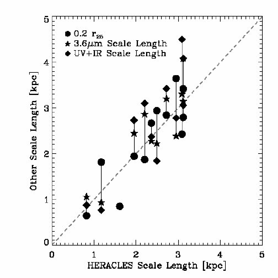
V.2. Scale Lengths At Other Wavelengths


Figure 33 shows the size of our galaxies at other wavelengths as a function of the exponential scale lengths that we measure from azimuthally averaged CO profiles, . Filled circles show , which Young et al. [42] found to be a typical scale length of CO emission. We observe the same here, with a scatter of . Stars show the exponential scale length fit to median profiles of m emission [21, from], a tracer of the distribution of old stellar mass. Diamonds plot the exponential scale length fit to profiles of star formation surface density, estimated from a combination of GALEX FUV emission and Spitzer 24m data [21, from]. All three quantities scatter about equality, with on average – lower than the other two, not a significant difference. The plot underscores the well-established close association between CO emission and stellar light in disk galaxies [41, 42, 25, e.g.,] and the similar match between the distributions of CO and star formation [21, e.g.,].
V.3. HERACLES CO and THINGS Hi Velocities


The THINGS data allow us to test our assumption that CO and H I have the same mean velocity (§III.2). To do so, we assemble a set of spatially independent spectra, each with peak SNR greater than . For each spectrum, we measure the intensity-weighted mean velocity of CO emission, , and extract the intensity-weighted mean H I velocity, , from the THINGS first moment maps [37].
The gray histogram in Figure 34 shows the distribution of for all spectra. The mean velocities of CO and H I appear closely matched for most spectra. A Gaussian fit to the distribution (thick dashed line) has width km s-1 and a center consistent with zero offset ( km s-1). The scatter in is much smaller than the – km s-1 width of our baseline fitting regions (§III.2), so the agreement is not a product of our reduction. The extended wings come almost entirely from a few inclined, massive spirals (NGC 2841, 2903, 3521, 7331), galaxies that also sometimes show multiple components in a single H I spectrum. These outliers are interesting, but here we emphasize the basic result that H I and CO gas show approximately the same mean velocity.
V.4. Comparison to CO Observations


CO emission has been mapped for many galaxies in our sample. Here we compare HERACLES to the FCRAO survey [42, resolution ], BIMA SONG [14], and the Nobeyama CO Atlas of Nearby Spiral Galaxies [18, resolution ]. We use two data sets drawn from BIMA SONG: on-the-fly maps made with the NRAO 12-m (resolution ) and the combined BIMA + 12-m data (typical resolution ). We refer to the former as the “NRAO 12-m” and the latter as BIMA SONG.
Our method of comparison is the following:
- 1.
We convolve each plane of each HERACLES data cube with a series of Gaussian kernels to create data cubes with angular resolutions of , , and , appropriate for comparison with Kuno et al. [18], the FCRAO survey, and the NRAO 12-m data. We convolve BIMA SONG to resolution in the same manner and compare it to HERACLES at this resolution.
- 2.
For each galaxy, we extract spectra from each data cube at a series of independent pointings. When comparing to the FCRAO survey, these are the FCRAO pointings, which are usually spaced by a full () beam width along the major axis. When comparing with Kuno et al. [18], BIMA SONG, and the NRAO 12-m, the pointings are on a grid that covers most of the galaxy with sampling points spaced by a full beam width — i.e., and .
- 3.
We smooth these spectra in velocity so that they all have comparable velocity resolution, km s-1 (chosen to match the FCRAO survey).
- 4.
We discard all spectra where the peak SNR is less than 5. When comparing with the FCRAO survey, we consider only pointings where Young et al. [42] report a peak temperature, mean velocity, and line width.
The result is a series of reasonably high SNR spectra at matched positions with matching angular and velocity resolutions. For each spectrum, we measure four parameters: the peak intensity of the line, (in K); the intensity-weighted mean velocity of the line, (in km s-1); the full width at half maximum of the line, (in km s-1); and the integrated intensity of the line, (in K km s-1). Because the FCRAO survey data are not electronically available, we use the values of these parameters reported by Young et al. [42].
V.4.1 CO Velocity and Line Width



| Quantity | FCRAO Survey | NRAO 12-m | BIMA SONG | Kuno et al. [18] |
|---|---|---|---|---|
| (km s-1)aaValues are mean difference (HERACLES - other survey) or ratio (HERACLES/other survey) giving equal weight to each galaxy. | -2.9 | 3.6 | 2.4 | -0.4 |
| ratio of aaValues are mean difference (HERACLES - other survey) or ratio (HERACLES/other survey) giving equal weight to each galaxy. | 1.01 | 1.05 | 1.18 | 0.93 |
| ratio of aaValues are mean difference (HERACLES - other survey) or ratio (HERACLES/other survey) giving equal weight to each galaxy. | 0.76 | 0.87 | 0.67 | 0.81 |
| ratio of aaValues are mean difference (HERACLES - other survey) or ratio (HERACLES/other survey) giving equal weight to each galaxy. | 0.71 | 0.87 | 0.84 | 0.74 |
The line width and mean velocity are not expected to vary strongly between the CO and transition. Therefore comparing our measurements of these quantities to those from earlier surveys allows a basic check on our data. Overall, this exercise confirms that we measure the same basic line shapes found by previous surveys at matched positions and resolution. We show this in the top two panels of Figure 35 and the first two lines of Table 4, which give mean velocity offset and line width ratio (with equal weight to each galaxy).
The top left panel of Figure 35 shows the distribution of differences between the intensity-weighted mean CO (HERACLES) velocity and the intensity-weighted mean CO velocity. Each comparison survey appears as a separate, normalized histogram. A thick dashed line shows a Gaussian fit to the average of the BIMA SONG, NRAO 12-m, and Kuno et al. [18] histograms. This Gaussian is centered at km s-1 and has width km s-1, identical with the uncertainties to what we found comparing CO to H I.
The top right panel of Figure 35 shows the FWHM line width, , from HERACLES measured as a function of from other surveys. Error bars show uncertainty, estimated by repeatedly adding the measured noise to each spectrum and re-measuring (without the FCRAO spectra, we cannot estimate uncertainties for these data). As with the mean velocity, there is general good agreement between HERACLES, BIMA SONG, the NRAO 12-m, and Kuno et al. [18]. There are systematic differences: BIMA SONG tends to show slightly lower line widths than the other data sets while the Kuno et al. [18] yield slightly higher line widths. These have magnitude and affect the intercomparison of CO data as much as the comparison between HERACLES and the other surveys.
The outlier this comparison is the FCRAO survey. These data do not agree as well with our own as the other three data sets. Specifically, there are several pointings where the mean velocity and line width disagree strongly with our data. Most of these locations also overlap with BIMA SONG or the Kuno et al. [18] survey and in these cases, these surveys also disagree with the FCRAO survey. We note that 1) the FCRAO survey is the only data set from which we do not ourselves measure the line parameters, so methodology may drive some of the difference; 2) these are the only data which are not maps, so it is not easy to tell whether pointing offsets may affect the comparison.
V.4.2 CO Line Ratio
| Galaxy | FCRAO Survey | NRAO 12-m | BIMA SONG | Kuno et al. [18] | OtherbbIntegrated intensity (not peak temperature) ratios drawn from the literature. References: NGC 628, NGC 3351, NGC 7331 — Braine et al. [4]; NGC 2903 — Jackson et al. [16]; NGC 6946 — Crosthwaite & Turner [7] |
|---|---|---|---|---|---|
| NGC 628 | 0.93 | 1.01 | |||
| NGC 2841 | 0.72 | ||||
| NGC 2903 | 0.91 | 0.90 | 0.68 | 0.82 | – |
| NGC 3184 | 0.59 | 0.60 | |||
| NGC 3351 | 0.50 | 0.62 | 0.59 | 0.95 | 1.65 |
| NGC 3521 | 1.14 | 0.81 | 0.59 | 0.86 | |
| NGC 4736 | 0.70 | 1.02 | 0.83 | 1.12 | |
| NGC 5055 | 0.71 | 0.77 | 0.64 | 0.79 | |
| NGC 6946 | 0.85 | 1.03 | 0.77 | 0.92 | |
| NGC 7331 | 0.82 | 0.79 | 0.60 |
The ratio of CO measured by HERACLES to CO emission measured by previous surveys reflects both the relative calibrations of the telescopes and the line ratio, , which depends on the optical depth and excitation temperature of the gas. Generally speaking, indicates warm, optically thin gas. Optically thick gas produces – with the value reflecting the temperature of the gas, though in low density regions the levels may not be populated according to local thermodynamic equilibrium [LTE; see, e.g., 11, for a more thorough discussion].
In the bottom left panel of Figure 35 we plot the peak temperatures measured by HERACLES (-axis) as a function of the peak temperature measured from other surveys at matched position and resolution (-axis). We use the peak temperature because it avoids any concern related to the line profile or range of integration. We do not plot error bars, but recall that our condition to include a spectrum in this analysis was that have SNR (meaning the statistical uncertainty on the ratio is always ). Table 5 compiles the average peak temperature ratio for each galaxy and survey and notes several measurements from the literature.
The ratios in Table 5 span –, with most values between and . These values agree with previous observations of the Milky Way and other galaxies. CO emission in the Milky Way comes mostly from optically thick regions and typical line ratios are – in the disk and towards the Galactic center [29, 23, 24]. In the central regions of other galaxies, Braine & Combes [3] found an average line ratio . Casoli et al. [6] compile observations on a number of galaxies and report typical values of in galaxy nuclei and – in galaxy disks.
If the gas is optically thick, a ratio of corresponds to an excitation temperature of K, to K, and to K. Higher excitation temperatures yield a line ratio . The average of all the values in Table 5 is , which is consistent with optically thick gas with an excitation temperature K. One should treat this temperature with caution: we do not constrain the optical depth (e.g., using one of the isotopes of CO) and we have no verification that our sources are in LTE, so sub-thermally excited, low-density envelopes — which are observed in Galactic GMCs — may lower the overall intensity ratio [30, e.g.,].
There is noticeable scatter among the peak temperatures ratios derived from different data sets for the same galaxy. Some scatter may arise from differences in resolutions or area considered (the set of spectra with peak SNR varies with comparison survey). If we ignore these explanations, Table 5 suggests that there are systematic calibration differences among the various surveys at the level and that the calibration of a given galaxy in a given survey is uncertain by . These uncertainties seem reasonable for millimeter line observations and agree with the scatter in comparisons with the FCRAO survey carried out by Helfer et al. [14, their Figure 51] and Kuno et al. [18, their Figure 1].
Because is observed to vary between the center and the disk in both the Milky Way and other galaxies, the bottom right panel of Figure 35 shows the ratio of in the two transitions as a function of galactocentric radius. This plot shows only data from HERACLES and Kuno et al. [18]. These data most closely match our own in observing strategy, instrumentation, and resolution making them the best option for this comparison. Black points connected by lines show the median ratio in bins with the first bin centered at . In the centers of galaxies, we observe the same trend noted by Casoli et al. [6] and found in the Milky Way: the ratio is high () in the center of the galaxy and then drops rapidly to , remaining almost constant at this value out to the edge of our comparison at . This constancy must be interpreted with care. By selecting only high significance spectra, we bias ourselves to bright regions. This may have the effect of creating a homogeneous data set while omitting lower intensity emission that accounts for a significant fraction of the emission at large radii.
VI. Summary


This paper presents the HERA CO-Line Extragalactic Survey (HERACLES), a new survey of CO emission from nearby galaxies obtained using the IRAM 30m. Because on-the-fly mapping mode with the multi-pixel HERA allows us to efficiently map large areas with good sensitivity and adequate resolution, HERACLES targets a wider area than previous surveys. Most maps extend to the edge of the optical disk, defined by the isophotal radius .
Our sample overlaps THINGS and SINGS, allowing easy comparison to data from radio to UV wavelengths. One application of this multiwavelength data allows us to automate our reduction. We use the mean H I velocity from THINGS as a prior to define baseline fitting regions and are thus able to reduce spectra in a robust, automated manner. We verify the assumption that CO and H I exhibit the same mean velocity by direct comparison of HERACLES and THINGS mean velocities, finding little or no systematic difference. We also confirm that our automated approach matches a by-hand reduction well.
We clearly detect 14 galaxies and place upper limits on CO emission from 4 low metallicity, irregular dwarf galaxies. For a Galactic CO-to-H2 conversion factor, the implied H2 masses are mostly – times the H I mass and – times the stellar mass. More detailed analysis of the relationship between H2, H I, stars, and star formation in our sample is presented elsewhere [1, 21].
We illustrate the distribution of CO in the detected galaxies via channel maps, azimuthally averaged profiles, and intensity maps. Where we find emission, the brightness is usually consistent with – of the area inside the beam being covered by Galactic GMCs, though in a few regions the implied surface density averaged over our pc beam exceeds that of a Galactic GMC. The line width and mean velocity that we derive agree reasonably with previous (CO ) surveys; systematic differences among surveys do exist, with magnitude –, but HERACLES never appears to be an outlier.
The ratio of CO intensity to CO intensity for high significance spectra lies mostly in the range – with an average value of , comparable to that found in the inner Milky Way. This could be produced by optically thick gas with an excitation temperature K, though this temperature should not be over-interpreted without constraints on the optical depth or applicability of LTE. This line ratio is higher () in the centers of galaxies and then roughly constant as a function of radius, though we caution that strong selection effects may be at work.
Our detections include high significance emission from the outer part of the star-forming disk in several galaxies. We also find bright CO emission associated with an H I filament outside the main disk of NGC 4736 (radius ). The azimuthally averaged intensity usually declines smoothly even beyond these detections and we are sensitive to only the most massive individual GMCs. Therefore we would expect to find many more such regions with improved sensitivity.
Although the channel and integrated intensity maps show a variety of morphologies, the azimuthally averaged profiles are well-described by exponential declines. The best-fit scale lengths range from – kpc and correlate closely with optical radius, near-IR (stellar mass) scale length, and UV+IR (star formation) scale length. These results are in good agreement with previous findings that CO emission closely follows both the stellar light and distribution of star formation on large scales. The exponential decline in CO brightness is a combination of decreasing maximum brightness of CO emission and a decreased filling fraction of bright CO emission at large radii.
References
- [1] Bigiel, F., Leroy, A., Walter, F., Brinks, E., de Blok, W. J. G., Madore, B., & Thornley, M. D. 2008, AJ, 136, 2846
- [2] Blitz, L. 1993, in Protostars and Planets III, ed. E. H. Levy & J. I. Lunine, 125–161
- [3] Braine, J., & Combes, F. 1992, A&A, 264, 433
- [4] Braine, J., Combes, F., Casoli, F., Dupraz, C., Gerin, M., Klein, U., Wielebinski, R., & Brouillet, N. 1993, A&AS, 97, 887
- [5] Braine, J., Ferguson, A. M. N., Bertoldi, F., & Wilson, C. D. 2007, ApJ, 669, L73
- [6] Casoli, F., Dupraz, C., Combes, F., & Kazès, I. 1991, A&A, 251, 1
- [7] Crosthwaite, L. P., & Turner, J. L. 2007, AJ, 134, 1827
- [8] Dame, T. M., Hartmann, D., & Thaddeus, P. 2001, ApJ, 547, 792
- [9] de Blok, W. J. G., Walter, F., Brinks, E., Trachternach, C., Oh, S.-H., & Kennicutt, R. C. 2008, AJ, 136, 2648
- [10] Désert, F. X., Bazell, D., & Boulanger, F. 1988, ApJ, 334, 815
- [11] Eckart, A., Downes, D., Genzel, R., Harris, A. I., Jaffe, D. T., & Wild, W. 1990, ApJ, 348, 434
- [12] Engargiola, G., Plambeck, R. L., Rosolowsky, E., & Blitz, L. 2003, ApJS, 149, 343
- [13] Fukui, Y., Mizuno, N., Yamaguchi, R., Mizuno, A., Onishi, T., Ogawa, H., Yonekura, Y., Kawamura, A., Tachihara, K., Xiao, K., Yamaguchi, N., Hara, A., Hayakawa, T., Kato, S., Abe, R., Saito, H., Mano, S., Matsunaga, K., Mine, Y., Moriguchi, Y., Aoyama, H., Asayama, S.-i., Yoshikawa, N., & Rubio, M. 1999, PASJ, 51, 745
- [14] Helfer, T. T., Thornley, M. D., Regan, M. W., Wong, T., Sheth, K., Vogel, S. N., Blitz, L., & Bock, D. C.-J. 2003, ApJS, 145, 259
- [15] Israel, F. P., de Graauw, T., van der Biezen, J., de Vries, C. P., Brand, J., Habing, H. J., Leene, A., van de Stadt, H., van Amerongen, J., Wouterloot, J. G. A., & Selman, F. 1984, A&A, 134, 396
- [16] Jackson, J. M., Eckart, A., Cameron, M., Wild, W., Ho, P. T. P., Pogge, R. W., & Harris, A. I. 1991, ApJ, 375, 105
- [17] Kennicutt, Jr., R. C., Armus, L., Bendo, G., Calzetti, D., Dale, D. A., Draine, B. T., Engelbracht, C. W., Gordon, K. D., Grauer, A. D., Helou, G., Hollenbach, D. J., Jarrett, T. H., Kewley, L. J., Leitherer, C., Li, A., Malhotra, S., Regan, M. W., Rieke, G. H., Rieke, M. J., Roussel, H., Smith, J.-D. T., Thornley, M. D., & Walter, F. 2003, PASP, 115, 928
- [18] Kuno, N., Sato, N., Nakanishi, H., Hirota, A., Tosaki, T., Shioya, Y., Sorai, K., Nakai, N., Nishiyama, K., & Vila-Vilaró, B. 2007, PASJ, 59, 117
- [19] Lebrun, F., Bennett, K., Bignami, G. F., Caraveo, P. A., Bloemen, J. B. G. M., Hermsen, W., Buccheri, R., Gottwald, M., Kanbach, G., & Mayer-Hasselwander, H. A. 1983, ApJ, 274, 231
- [20] Leroy, A., Bolatto, A., Walter, F., & Blitz, L. 2006, ApJ, 643, 825
- [21] Leroy, A. K., Walter, F., Brinks, E., Bigiel, F., de Blok, W. J. G., Madore, B., & Thornley, M. D. 2008, AJ, 136, 2782
- [22] Mangum, J. G., Emerson, D. T., & Greisen, E. W. 2007, A&A, 474, 679
- [23] Oka, T., Hasegawa, T., Handa, T., Hayashi, M., & Sakamoto, S. 1996, ApJ, 460, 334
- [24] Oka, T., Hasegawa, T., Hayashi, M., Handa, T., & Sakamoto, S. 1998, ApJ, 493, 730
- [25] Regan, M. W., Thornley, M. D., Helfer, T. T., Sheth, K., Wong, T., Vogel, S. N., Blitz, L., & Bock, D. C.-J. 2001, ApJ, 561, 218
- [26] Rickard, L. J., Palmer, P., Morris, M., Turner, B. E., & Zuckerman, B. 1975, ApJ, 199, L75
- [27] Rosolowsky, E. 2007, ApJ, 654, 240
- [28] Sakamoto, K., Okumura, S. K., Ishizuki, S., & Scoville, N. Z. 1999, ApJS, 124, 403
- [29] Sakamoto, S., Hasegawa, T., Hayashi, M., Handa, T., & Oka, T. 1995, ApJS, 100, 125
- [30] Sakamoto, S., Hayashi, M., Hasegawa, T., Handa, T., & Oka, T. 1994, ApJ, 425, 641
- [31] Schuster, K.-F., Boucher, C., Brunswig, W., Carter, M., Chenu, J.-Y., Foullieux, B., Greve, A., John, D., Lazareff, B., Navarro, S., Perrigouard, A., Pollet, J.-L., Sievers, A., Thum, C., & Wiesemeyer, H. 2004, A&A, 423, 1171
- [32] Schuster, K. F., Kramer, C., Hitschfeld, M., Garćıa-Burillo, S., & Mookerjea, B. 2007, A&A, 461, 143
- [33] Solomon, P. M., & de Zafra, R. 1975, ApJ, 199, L79
- [34] Solomon, P. M., Rivolo, A. R., Barrett, J., & Yahil, A. 1987, ApJ, 319, 730
- [35] Strong, A. W., Bloemen, J. B. G. M., Dame, T. M., Grenier, I. A., Hermsen, W., Lebrun, F., Nyman, L.-A., Pollock, A. M. T., & Thaddeus, P. 1988, A&A, 207, 1
- [36] Strong, A. W., & Mattox, J. R. 1996, A&A, 308, L21
- [37] Walter, F., Brinks, E., de Blok, W. J. G., Bigiel, F., Kennicutt, R. C., Thornley, M. D., & Leroy, A. 2008, AJ, 136, 2563
- [38] Walter, F., Taylor, C. L., Hüttemeister, S., Scoville, N., & McIntyre, V. 2001, AJ, 121, 727
- [39] Wilson, B. A., Dame, T. M., Masheder, M. R. W., & Thaddeus, P. 2005, A&A, 430, 523
- [40] Wilson, R. W., Jefferts, K. B., & Penzias, A. A. 1970, ApJ, 161, L43+
- [41] Young, J. S., & Scoville, N. Z. 1991, ARA&A, 29, 581
- [42] Young, J. S., Xie, S., Tacconi, L., Knezek, P., Viscuso, P., Tacconi-Garman, L., Scoville, N., Schneider, S., Schloerb, F. P., Lord, S., Lesser, A., Kenney, J., Huang, Y.-L., Devereux, N., Claussen, M., Case, J., Carpenter, J., Berry, M., & Allen, L. 1995, ApJS, 98, 219