Estimating Trees from Filtered Data: Identifiability of Models for Morphological Phylogenetics

Elizabeth S. Allman Address: Department of Mathematics and Statistics, University of Alaska Fairbanks, PO Box 756660, Fairbanks, AK 99775, U.S.A Mark T. Holder Address: Department of Ecology and Evolutionary Biology, University of Kansas, 1200 Sunnyside Avenue, Lawrence, Kansas 66045, U.S.A John A. Rhodes Address: Department of Mathematics and Statistics, University of Alaska Fairbanks, PO Box 756660, Fairbanks, AK 99775, U.S.A

Abstract

As an alternative to parsimony analyses, stochastic models have been proposed (Lewis, 2001; Nylander et al., 2004) for morphological characters, so that maximum likelihood or Bayesian analyses may be used for phylogenetic inference. A key feature of these models is that they account for ascertainment bias, in that only varying, or parsimony-informative characters are observed. However, statistical consistency of such model-based inference requires that the model parameters be identifiable from the joint distribution they entail, and this issue has not been addressed.

Here we prove that parameters for several such models, with finite state spaces of arbitrary size, are identifiable, provided the tree has at least $8$ leaves. If the tree topology is already known, then $7$ leaves suffice for identifiability of the numerical parameters. The method of proof involves first inferring a full distribution of both parsimony-informative and non-informative pattern joint probabilities from the parsimony-informative ones, using phylogenetic invariants. The failure of identifiability of the tree parameter for $4$ -taxon trees is also investigated.

Keywords:

maximum likelihood , morphology , parsimony-informative , Mkv Model

2008 MSC

92D15 , 60J20 , 62M99

1 Introduction

Currently, the vast majority of phylogenetic inference from morphological data is based on the parsimony criterion – the preference for the phylogeny that can explain the data with the fewest number of changes in character states. Lewis (2001) discussed the obstacles to the application of Markov models for phylogenetic inference to discrete morphological data. He argued that, despite its limitations, the simplest continuous-time Markov model offers advantages over relying solely on parsimony. He referred to this model as the M $k$ model, for “Markov” with $k$ -states. The M $k$ model is a generalization of some of the earliest models used in phylogenetics by Jukes and Cantor (1969), Neyman (1971), Farris (1973), and Cavender (1978); it assumes that all states have the same frequency and all transitions between different states occur at the same rate. Maximum likelihood (ML) inference under the M $k$ model should be able to infer trees more accurately than parsimony, because use of the M $k$ model allows one to take into account that some branches on the tree may be longer than others. This branch length heterogeneity could arise from differences in the temporal duration of branches, differences in the rate of character evolution, or both. Parsimony does not attempt to correct for the fact that convergent changes may not be equally likely to occur on every branch of the tree; as a result, it has been shown to be susceptible to “long-branch attraction” when branch-length heterogeneity is present (Felsenstein, 1978).

As Lewis (2001) pointed out, complications arise when applying the M $k$ model to morphological characters. The definitions of both characters (also referred to as “transformation series”) and character states are problematic in morphological systematics. Systematists disagree about the most appropriate meanings of concepts such as homology (Sereno, 2007; Rieppel and Kearney, 2007; Wiley, 2008, cf. ) which are crucial to character coding. Even if one chooses a particular definition of homology, doing so does not establish a clear-cut set of rules for “atomizing” the complete morphology of an organism to a set of characters that can be treated as independent instances of a general model of character evolution (but see Ramirez, 2007, for one example of an attempt to create an objective system for character coding). While there are rarely clear criteria for delimiting character states or identifying homologous traits between species, systematists try to find traits that can be cleanly scored into one of a few discrete bins. For example, the degree contact of bones in the skull could be scored as a $2$ -state character with state 0 representing “not touching” and state 1 representing “in contact.” If these characters are heritable and do not change too quickly over evolutionary time, then even simple, discrete-state coding scheme can provide information about evolutionary relationships. Of particular concern here is the fact that variation across the taxa under investigation is vital to the process of recognizing characters and character states. This means that it is not appropriate to view the coded character matrix as a random sampling of characters generated by the evolutionary process, since it is biased to contain characters thought to be phylogenetically useful. Such ascertainment bias, in which the collected data fails to be representative of the entire population of characters, must be corrected for in a valid statistical analysis.

It is difficult to precisely describe the biases inherent in the process of the coding of morphological traits into columns of a data matrix. For one thing, it is relatively rare for systematists to even report their methods for excluding potential characters from consideration; Poe and Wiens (2000) found that fewer than 20% of papers in morphological systematics reported such criteria. The requirement that there be variability among the taxa of interest is clearly one important aspect of character coding. As noted by Sereno (2007), several definitions of “character” or “homology” given by systematists include the idea that a character differentiates between taxa. For example he pointed out the following definitions of “character” in systematics:

•

“Any attribute of an organism or a group of organisms by which it differs from an organism belonging to a different category or resembles an organism of the same category” (Mayr et al., 1953, p. 315,)
•

“We will call those peculiarities that distinguish a semaphoront (or a group of semaphoronts) from other semaphoronts ‘characters’ $\ldots$ ”(Hennig, 1966, p. 7,)
•

“an observation that captures distinguishing peculiarities among organisms $\ldots$ ” (Rieppel and Kearney, 2002)

The emphasis on variability among taxa means that constant characters generally do not appear in morphological character matrices. When they do occur, it is often the result of pruning the list of taxa (the characters had been chosen because of variation among members of a larger set of taxa). As Lewis (2001) noted, this bias cannot be corrected by morphologists changing their systems for encoding characters. How many constant characters should be encoded to represent a complex feature that is identical across a set of taxa? The question seems intractable because there are no strict rules about how many aspects of a trait should be coded as independent characters.

The absence of constant characters is the most obvious effect of the ascertainment biases in the coding of morphological data matrices. Lewis (2001) proposed a corrected model, M $k$ v, which can be used to calculate a likelihood from a data set conditional on the fact that only variable characters are sampled (Felsenstein, 1992, see also).

Nylander et al. (2004) further noted that many morphological matrices only contain parsimony-informative characters. A parsimony-informative character is one which does not have the same parsimony score on every tree. In order for a character to be parsimony-informative, it must have more than one character state that is shared by multiple taxa. For instance, if a character ‘wing shape’ for a collection of insects has 3 states, and there is exactly one taxon with shape 2 and one with shape 3, with all others having shape 1, then the character is variable, but not parsimony-informative. If, one the other hand, at least two taxa have shape 1 and at least 2 taxa have shape 2, then the character is parsimony-informative.

If parsimony-noninformative characters are avoided in the process of character coding, then one has data from a smaller set of characters than for the M $k$ v model and should condition the likelihood calculations based on the parsimony-informative ascertainment bias. We will refer to this model as $\text{M$k$}_{\text{pars-inf}}$ . It was introduced by Nylander et al. (2004), and implemented in the freely available software, MrBayes (Ronquist and Huelsenbeck, 2003).

The use of the M $k$ v and $\text{M$k$}_{\text{pars-inf}}$ model in phylogenetic inference has grown steadily. Dozens of studies using these models have now been published. Unfortunately, in many cases, authors do not report which form of conditioning is used during analyses, so it is impossible to ascertain the relative frequency of the M $k$ v model compared to the $\text{M$k$}_{\text{pars-inf}}$ model.

The statistical inconsistency of parsimony as an estimator of phylogenetic trees was one of Lewis’s (2001) primary reasons for proposing the M $k$ v model as an improved basis of inference. However, Lewis (2001) did not prove that ML inference using the M $k$ v model is a consistent estimator of the phylogeny. Nor did Nylander et al. (2004) prove the consistency of ML inference under the $\text{M$k$}_{\text{pars-inf}}$ model.

Recall that statistical consistency of a method of inference under a model means that if data is generated according to the model, then as the amount of data grows, the probability of inferring the correct model parameters (e.g., the tree topology and numerical parameters such as edge lengths) approaches 1. There is a standard approach to proving consistency under maximum likelihood (Wald, 1949) that reduces the issue to proving the model has identifiable parameters. This means the crucial step is to show that any two different choices of model parameters lead to a different distribution of data. Identifiability of model parameters is equally essential for their inference in Bayesian analyses, and non-identifiability of parameters that are not the focus of such an analysis may also be problematic (Rannala, 2002).

The identifiability of the M $k$ model can be proved through arguments based on an appropriate generalization of the Jukes-Cantor distance. However, the question that we address is whether we can identify the tree and model parameters when the data is filtered to contain only variable patterns, or only parsimony-informative patterns. This filtering greatly changes the problem, so that a straightforward modification of the proof for M $k$ to $\text{M$k$}_{\text{pars-inf}}$ fails. One instance of the question of tree identifiability using only parsimony-informative pattern frequencies was investigated by Steel et al. (1993). Although that paper is focused on other issues, in the appendix it is shown that for the CFN model on 4-taxon trees, several explicit choices of edge lengths on different tree topologies can lead to identical distributions of parsimony-informative (and constant) patterns.

Here we demonstrate that the tree topology is identifiable under the M $k$ v model under sufficiently broad circumstances to justify its use in data analysis. While we show that under the $\text{M$k$}_{\text{pars-inf}}$ model, $k\geq 2$ , the tree topology is not identifiable for 4-taxon trees, more importantly we establish that the tree topology is identifiable when eight or more taxa are involved. Moreover, if the tree is known, then the branch lengths are identifiable on trees of seven or more taxa. (The need for seven or eight taxa in these statements may be an artifact of our methods; we do not fully analyze the cases of trees with five, six, or seven taxa.)

Our results are actually valid for more general models, the variable-patterns-only and parsimony-informative-patterns-only versions of the $k$ -state general Markov model GM $k$ , a generalization of the M $k$ model in which the transition probabilities on edges are not constrained to be equal among the different states. The identifiability of the tree topology for the unfiltered GM $k$ was proven by Steel (1994), and the identifiability of all numerical parameters for this model by Chang (1996). Identifiability results for a 2-class mixture model of GM $k$ with invariable sites (GM $k$ +I) were investigated by Allman and Rhodes (2008a). That model is quite closely related to a variable-patterns-only model, as the invariable class essentially makes direct observation of constant patterns from variable characters impossible. Our results here in fact imply strengthenings of some of the theorems in Allman and Rhodes (2008a). Furthermore, since the general Markov model includes as submodels the general time-reversible models with fixed rate-matrices describing the substitution process across the tree, our results apply to the filtered versions of those models as well.

Interestingly, one implication of this work and that of Steel et al. (1993) which seems not to have been widely noticed, is that the most basic example used to explain phylogenetic inference to students is actually an example of an intractable problem. Assuming any model encompassing the M $k$ model underlies the data, if we attempt to infer an unrooted four-leaf tree using only those characters that are parsimony-informative, then no method of inference can consistently identify the correct tree, even if given an infinite sample of characters. We establish that each of the three possible binary tree topologies can lead to all possible positive distributions of parsimony-informative patterns, thus strengthening the result of Steel et al. (1993).

We emphasize that the non-identifiability in this case is not an argument for ignoring the ascertainment bias. If characters are filtered to contain only parsimony-informative patterns and the ascertainment bias is ignored then inference can be positively misleading in the sense that Felsenstein (1978) used the phrase – the incorrect tree can be preferred with increasing support as the number of characters increases. Indeed, using standard software to perform a maximum likelihood analysis of filtered 4-taxon data under the misspecified M $k$ model often results in the erroneous inference of a particular tree topology. While maximum likelihood inference under the correctly-specified $\text{M$k$}_{\text{pars-inf}}$ model does not prefer any tree topology, it will at least not lead to rejection of the true tree (except when some parsimony-informative patterns do not occur, due to sampling error).

We also note that the M $k$ v and $\text{M$k$}_{\text{pars-inf}}$ models may be appropriate in contexts outside of morphological systematics. For example, one (admittedly flawed) method for incorporating information from insertion/deletion events (indels) in a molecular sequence analysis is to code the absence or presence of a base as a 0/1 character. Because columns without indels are generally not coded, and columns in which all taxa lack a nucleotide are impossible to correctly code, such binary characters should be analyzed under a model that conditions on the variability of the characters. (More appropriate ways of modeling indels are discussed by Thorne et al. (1991) and Diallo et al. (2007).) In a similar vein, one of the models included in our analysis, GM2v, the variable-patterns-only version of the model GM2, has recently been used for a likelihood analysis of intron loss and gain by Csűrös et al. (2007).

Finally, we emphasize that while establishing identifiability of parameters for a model is essential for its use in statistical inference, there are other important issues that we do not address in this work. In particular, efficiency concerns how many characters are needed for inference by a particular method such as maximum likelihood to perform well, and robustness concerns how well the method performs on data deviating from the assumed model. Even for unfiltered phylogenetic models these questions have mainly been investigated by simulation, rather than theoretically.

2 Parsimony-informative models

The models of sequence evolution we consider are submodels of the general Markov model, with observations restricted to variable or parsimony-informative patterns. In this section, we make this more precise.

By an $n$ -taxon tree $T$ , we mean an unrooted, $n$ -leaf, topological phylogenetic tree, with leaves labeled by the taxa $a_{i}$ , $i\in[n]$ . We do not assume the tree $T$ is binary; it need not be fully resolved. However, we do assume $T$ has no internal nodes of valence $2$ .

The $k$ -state general Markov substitution model, GM $k$ , on $T$ is parameterized as follows: First, arbitrarily choose some node of $T$ to be the root. Designating character states by elements of $[k]=\{1,2,\dots,k\}$ , a row vector $\boldsymbol{\pi}=(\pi_{i})\in[0,1]^{k}$ , with entries summing to 1, gives probabilities of each state $i\in[k]$ occurring at the root. On each edge $e$ of $T$ , directed away from the root, a $k\times k$ Markov matrix $M_{e}$ , with rows summing to 1, gives conditional probabilities of each possible state change occurring on that edge. We refer to the entries of $\boldsymbol{\pi}$ and the $M_{e}$ as the numerical parameters of GM $k$ , in contrast to the tree parameter $T$ , which is non-numerical.

Throughout, we assume that

(1)

all entries of $\boldsymbol{\pi}$ and the $M_{e}$ are strictly positive, and
(2)

all $M_{e}$ are non-singular.

Condition (1) is a biologically natural one, implying that all states and all state transitions can occur. It also ensures that, the probability distribution arising for one choice of the root of $T$ and numerical parameters is identical to one for any other choice of the root, with a corresponding appropriate choice of numerical parameters that are unique up to permutations of character states at internal nodes of $T$ (Steel et al., 1994; Allman and Rhodes, 2003). This means that identifiability of numerical parameters for GM $k$ can only be claimed up to the arbitrary choices of the root and orderings of states at internal nodes. Condition (2), which when restricted to continuous-time models is just the requirement that edge lengths be finite, is needed to avoid other sources of non-identifiability (such as a situation in which all terminal edges have infinite length, so that no information about internal tree structure is retained in the joint distribution).

Following Lewis (2001), we use M $k$ to denote the submodel of GM $k$ which assumes a uniform root distribution, $\boldsymbol{\pi}=(1/k,\dots,1/k)$ , and that for each Markov matrix all off-diagonal entries are equal. Thus M4 is also known as the Jukes-Cantor (JC) model, while M2 is the Cavender-Farris-Neyman (CFN) model. While Lewis (2001) presents a continuous-time formulation of this model, that is equivalent to the submodel of the one given here by making an additional assumption that off-diagonal matrix entries are smaller than diagonal entries. As our methods are primarily algebraic, we do not focus on the continuous-time formulation.

For the GM $k$ (or M $k$ ) model on a fixed $n$ -taxon tree $T$ , the joint probability distribution of character states at the leaves of the $T$ can be expressed by polynomial formulas in the entries of $\boldsymbol{\pi}$ and the $M_{e}$ . Denote a pattern of states at the leaves of a tree by a vector $\mathbf{i}=(i_{1},i_{2},\dots,i_{n})=i_{1}i_{2}\dots i_{n}\in[k]^{n}$ , where the leaf labeled by taxon $a_{j}$ displays state $i_{j}$ . We use $p_{\mathbf{i}}$ to denote the probability of observing pattern $\mathbf{i}$ that arises from a specific model, tree, and numerical parameters.

We wish to modify the above models to describe data that is collected only on parsimony-informative patterns. We will not explicitly treat a variable-patterns-only model, as the necessary modifications are straightforward.

Denote the set of parsimony-informative patterns by

\mathcal{I}=\{\mathbf{i}={i_{1}i_{2}i_{3}\cdots i_{n}}~|~i_{j_{1}}=i_{j_{2}}\neq i_{j_{3}}=i_{j_{4}},\ \text{for some distinct $j_{l}$}\}.

For fixed $k$ , the total number of patterns grows exponentially with $n$ , while the number of parsimony-noninformative ones grow only polynomially. Thus the cardinality of $\mathcal{I}$ grows exponentially with $n$ .

Suppose that from a total number of $M$ independent, identically distributed characters described by the GM $k$ model, we may obtain only data counts $n_{\mathbf{i}}$ for those patterns $\mathbf{i}\in\mathcal{I}$ . Since assumption (1) implies $p_{\mathbf{i}}>0$ for all $\mathbf{i}$ , we have that

\mathcal{P}(n_{\mathbf{i}}>0\text{ for some }\mathbf{i}\in\mathcal{I})\to 1\text{ as }M\to\infty.

With $N=\sum_{\mathbf{i}\in\mathcal{I}}n_{\mathbf{i}}$ , the total count of observed characters, then $N\leq M$ and $\mathcal{P}(N>0\text{)}\to 1$ as $M\to\infty$ .

If we were able to observe all patterns, including parsimony-noninformative ones, then observed pattern frequencies would be $\hat{p}_{\mathbf{i}}={n_{\mathbf{i}}}/M,$ which, by the strong law of large numbers converges to $p_{\mathbf{i}}$ almost surely as $M\to\infty$ . However, since $M$ is unknown from data, we cannot compute $\hat{p}_{\mathbf{i}}$ directly for $\mathbf{i}\in\mathcal{I}$ . We instead introduce the observed frequencies

\hat{q}_{\mathbf{i}}=\frac{n_{\mathbf{i}}}{N}.

These are estimators for conditional probabilities, $q_{\mathbf{i}}$ , that one observes $\mathbf{i}$ given that a parsimony-informative pattern is observed. Thus

q_{\mathbf{i}}=\mathcal{P}(\mathbf{i}~|~\text{pattern is parsimony-informative})=\frac{p_{\mathbf{i}}}{p},

(1)

where

p=\mathcal{P}(\text{pattern is parsimony-informative})=\sum_{\mathbf{i}\in\mathcal{I}}p_{\mathbf{i}}.

Note that $\hat{q}_{\mathbf{i}}\to q_{\mathbf{i}}$ almost surely as $M\to\infty$ .

We thus define a parameterized model, $\text{GM$k$}_{\text{pars-inf}}$ , which gives values of the $q_{\mathbf{i}}$ , $\mathbf{i}\in\mathcal{I}$ , as a function of the usual GM $k$ parameters. For any fixed tree, explicit formulas for the $q_{\mathbf{i}}$ as rational functions of the numerical model parameters are easily obtained. Restricting to any submodel of GM $k$ , we similarly obtain a parsimony-informative version of the submodel. For instance, $\text{M$k$}_{\text{pars-inf}}$ denotes the model describing the restriction of observations of the M $k$ model to parsimony-informative patterns.

Similarly, one can define parameterized models GM $k$ v and M $k$ v in which the non-constant patterns can be observed, by conditioning on the variableness of patterns rather than their parsimony-informativeness.

3 Results

As mentioned, Steel et al. (1993) showed that from parsimony-informative patterns alone the tree topology is not identifiable for the CFN (i.e., M2) model on a 4-taxon tree, at least for certain parameter choices. We begin by extending this negative result to models with more character states, and to the full parameter space.

Consider the model $\text{M$k$}_{\text{pars-inf}}$ on a 4-leaf tree $a_{1}a_{2}|a_{3}a_{4}$ . Since there are $3k(k-1)$ parsimony-informative patterns for the $k$ -state model, a probability distribution arising from this model is represented by a vector of $3k(k-1)$ probabilities. However, these vector entries are all the same for patterns of the same form (i.e, $q_{xxyy}$ is the same for all choices of distinct states $x$ and $y$ , etc.). Thus the distribution can be represented by a vector

\vec{Q}=(Q_{xxyy},Q_{xyyx},Q_{xyxy}),

where $Q_{xxyy}=k(k-1)q_{xxyy}$ , etc., so that

Q_{xxyy}+Q_{xyxy}+Q_{xyyx}=1.

In 3-space, $\vec{Q}$ lies on the part of the plane $x+y+z=1$ in the non-negative octant. This set, the probability simplex $\Delta$ , is an equilateral triangular patch, with corners $(1,0,0)$ , $(0,1,0)$ , and $(0,0,1)$ .

Theorem 1.

The set of all probability distributions arising from the model $\text{M$k$}_{\text{pars-inf}}$ with positive probabilities of a substitution on each edge of the binary tree $a_{1}a_{2}|a_{3}a_{4}$ is precisely the interior of $\Delta$ .

As the set of probability distributions described in the theorem is independent of the tree topology, we immediately obtain the following.

Corollary 2.

Suppose $T$ is a 4-taxon tree. Then the topology of $T$ is not identifiable for the model $\text{M$k$}_{\text{pars-inf}}$ or $\text{GM$k$}_{\text{pars-inf}}$ , for any $k\geq 2$ .

Corollary 3.

Suppose data is generated by the $\text{M$k$}_{\text{pars-inf}}$ or $\text{GM$k$}_{\text{pars-inf}}$ model, on a 4-taxon tree with parameters resulting in a positive probability of observing every parsimony-informative pattern. Then any method of inference of the tree topology either (a) always returns all three trees, or (b) can be positively misleading.

The proof of Theorem 1 given in Appendix A uses explicit calculations and topological arguments.

Note that standard numerical maximum likelihood software generally infers a particular tree topology when 4-taxon data produced by the $\text{M$k$}_{\text{pars-inf}}$ model is analyzed under the misspecified M $k$ model. Thus this model misspecification can lead to positively misleading inference.

For larger trees, one might expect that omitting parsimony-noninformative data would result in little loss of information. To establish positive results on the identifiability of parameters for the models $\text{GM$k$}_{\text{pars-inf}}$ and $\text{M$k$}_{\text{pars-inf}}$ , we focus on $\text{GM$k$}_{\text{pars-inf}}$ , since results about it apply to its submodels. We separately address the identifiability of the tree topology and identifiability of the numerical model parameters, since the tree topology must be fixed before the numerical parameters are even meaningful.

Theorem 4.

Suppose $n\geq 8$ . Then any $n$ -taxon tree topology is identifiable for the $\text{GM$k$}_{\text{pars-inf}}$ model, and its submodels, such as $\text{M$k$}_{\text{pars-inf}}$ .

Note that we do not claim $n=8$ is the minimal number of taxa ensuring identifiability for either $\text{GM$k$}_{\text{pars-inf}}$ or $\text{M$k$}_{\text{pars-inf}}$ , either for all $k$ or for any fixed choice. Our method of proof simply does not apply when $n\leq 7$ .

Since from a distribution for the GM $k$ v model one may compute that of the $\text{GM$k$}_{\text{pars-inf}}$ model with the same parameters, we immediately obtain the following.

Corollary 5.

Suppose $n\geq 8$ . Then any $n$ -taxon tree topology is identifiable for the GM $k$ v model, and its submodels, such as M $k$ v.

The proof of Theorem 4 is given in Appendix B, and depends on the construction of phylogenetic invariants for $\text{GM$k$}_{\text{pars-inf}}$ (i.e., polynomials that vanish on any joint distribution of patterns for $\text{GM$k$}_{\text{pars-inf}}$ arising from a fixed tree topology). These invariants are close in spirit to an encoding of the well-known 4-point condition of Buneman (1971), using the log-det distance (Cavender and Felsenstein, 1987; Steel, 1994), but the restriction to parsimony-informative patterns introduces complications.

Assuming the tree topology is already known, we next consider the identifiability of numerical parameters. Although our result on identifiability of the tree topology required at least 8 taxa, fewer taxa suffice for our remaining arguments.

For small trees, though, there are certainly instances of non-identifiability. For instance, in the 4-taxon case, for either of the models $\text{GM2}_{\text{pars-inf}}$ or $\text{M2}_{\text{pars-inf}}$ , we cannot have identifiability of numerical parameters. The easiest way to see this is a dimension count: There are only 6 parsimony-informative patterns for $\text{GM2}_{\text{pars-inf}}$ on a 4-taxon tree, yet the model has 11 free numerical parameters. However, the continuous parameterization of the model cannot injectively map any full-dimensional subset of $\mathbb{R}^{11}$ into a 5-dimensional subspace of $\mathbb{R}^{6}$ . In fact, any distribution arising from the model must arise from infinitely many choices of parameters. Similarly, the model $\text{M2}_{\text{pars-inf}}$ on a 4-taxon tree has 5 free numerical parameters, but up to symmetry there are only 3 parsimony-informative patterns.

In Appendix C we give the outline of the proof of the following, though the work of Appendix E is needed to complete the argument.

Theorem 6.

Suppose $n\geq 7$ and $T$ is a known $n$ -taxon tree. Then numerical parameters of the model $\text{GM$k$}_{\text{pars-inf}}$ , and its submodels, such as $\text{M$k$}_{\text{pars-inf}}$ , on $T$ are identifiable, up to choice of a root for $T$ and permutation of the states at the internal nodes of $T$ .

The issue of identifiability of GM parameters only up to a permutation of states at internal nodes of $T$ is a well-known one (Allman and Rhodes, 2003), arising because the joint distribution gives no information on which hidden state is which. Chang (1996) removed this ambiguity through a biologically-motivated assumption that all Markov matrices have their largest entries in each row appearing on the diagonal. As permuting the states at internal nodes has the effect of reordering the rows and columns of the Markov matrices, the highly-structured pattern of entries in the Markov matrices for M $k$ enables one to remove the ambiguity even without Chang’s assumption. Thus the identifiability of numerical parameters for the $\text{M$k$}_{\text{pars-inf}}$ model is, in fact, complete.

For trees with fewer than $7$ taxa, we obtain a slightly weaker result on identifiability of numerical parameters, as stated and proved in Appendix D. Although that result is perhaps of less interest for biological application, we include it as it provides a good introduction to the method of proof of Theorem 6. These proofs again depend on phylogenetic invariants, but invariants not for the model $\text{GM$k$}_{\text{pars-inf}}$ , but rather for GM $k$ (Allman and Rhodes, 2008b; Allman and Rhodes, 2007). These invariants lead to algebraic formulas for determining the values of $p_{\mathbf{i}}$ for all $\mathbf{i}\in[k]^{n}$ from the values of $q_{\mathbf{i}}$ for those $\mathbf{i}\in\mathcal{I}$ . Then the identifiability of parameters for the GM $k$ model established by Chang (1996) completes the proof.

An interesting aspect of the work in Appendix D is that our arguments for the $\text{M2}_{\text{pars-inf}}$ model on 5-taxon trees establish parameter identifiability for generic parameter choices, but fail under a molecular clock assumption. Thus what one might consider the simplest assumption actually leads to a more difficult mathematical analysis, due to the symmetries inherent in it.

4 Acknowledgements

The authors thank the Isaac Newton Institute, and the organizers of its Fall 2007 programme in Phylogenetics, for funding enabling the visits where this work was begun. MTH thanks the University of Kansas for travel funds to attend the INI. Funds from the National Science Foundation, grant DMS 0714830, made these visits possible for ESA and JAR, as well as supported the conclusion of the research.

All authors contributed equally to this work.

Appendix A Non-identifiability of 4-taxon trees

Our proof of Theorem 1 will require the notion of the the fundamental group of a space, from algebraic topology. As this does not commonly appear in the phylogenetics literature, Massey (1991) provides a good development for those unfamiliar with it. The arguments in this appendix have little in common with those of the rest of the paper, so readers interested primarily in other results may elect to move on to Appendix B.

Recall $\Delta$ denotes the 2-dimensional probability simplex, as defined in Section 3. To simplify some formulas, it will be convenient to represent a vector $\vec{Q}=(Q_{1},Q_{2},Q_{3})\in\Delta$ by homogeneous coordinates $[Q_{1},Q_{2},Q_{3}]$ which are not all zero and are determined only up to rescaling by a non-zero constant. That is, $[Q_{1},Q_{2},Q_{3}]=[\lambda Q_{1},\lambda Q_{2},\lambda Q_{3}]$ for any $\lambda\neq 0$ . Thus $[Q_{1}^{\prime},Q_{2}^{\prime},Q_{3}^{\prime}]$ represents $\vec{Q}$ with $Q_{i}=Q_{i}^{\prime}/(Q_{1}^{\prime}+Q_{2}^{\prime}+Q_{3}^{\prime})$ .

Associate to each of the five edges of the tree $a_{1}a_{2}|a_{3}a_{4}$ a parameter giving the probability of a substitution occurring on that edge, with $s_{1},s_{2},s_{3},s_{4}$ denoting the parameters on pendant edges leading to taxa $a_{1},a_{2},a_{3},a_{4}$ , respectively, and $s_{5}$ the parameter on the central edge. Thus the Markov matrix $M_{i}$ has diagonal entries $1-s_{i}$ and off-diagonal entries $s_{i}/(k-1)$ . We focus on the subset of the parameter space defined by

S=\left\{(s_{1},s_{2},s_{3},s_{4},s_{5})~|~s_{i}\in\left(0,1-1/k\right)\right\},

which corresponds to finite, positive edge lengths. However, for technical reasons we will also need to consider the extension of the parameterization to the larger set

S^{\prime}=\left\{(s_{1},s_{2},s_{3},s_{4},s_{5})~|~s_{i}\in\left[0,1-1/k\right),\text{ and either }s_{5}>0\text{ or two }s_{i}>0\right\}.

We let

\phi:S^{\prime}\to\Delta

denote the (extended) parameterization map giving $\vec{Q}$ as a function of the 5 edge probabilities.

For any $\epsilon>0$ , let $D_{\epsilon}=\{\vec{Q}\in\Delta~|~\min Q_{i}<\epsilon\}$ denote an open neighborhood in $\Delta$ of $\partial\Delta$ , the boundary of $\Delta$ . We also use $\partial\Delta$ to denote a loop, starting and ending at $[1,0,0]$ , parameterizing $\partial\Delta$ in the counterclockwise direction in Figure 1.

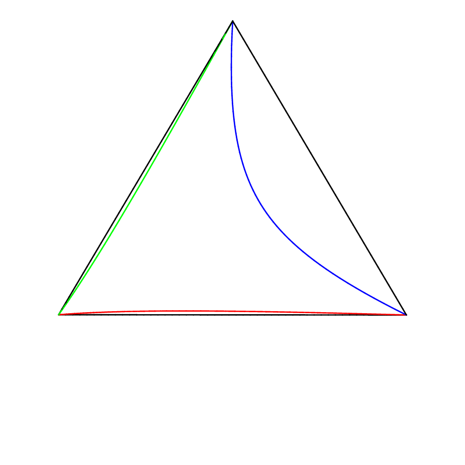
Refer to caption — Figure 1: The two-dimensional probability simplex $\Delta$ , with vertices $[1,0,0]$ (bottom left), $[0,1,0]$ (bottom right), and $[0,0,1]$ (top). The three curves form the loop $\phi\circ\gamma$ constructed in Lemma 7, for $k=4$ and $\delta=0.3$ , with the image of $\phi\circ\gamma_{1}$ in red, $\phi\circ\gamma_{2}$ in blue, and $\phi\circ\gamma_{3}$ in green. For smaller $\delta$ , the loop would be closer to the boundary of $\Delta$ .

Lemma 7.

For any $\epsilon>0$ , there exists a loop $\gamma$ in $S^{\prime}$ such that $\phi\circ\gamma$ is a loop in $D_{\epsilon}$ , starting and ending at $[1,0,0]$ , that is homotopic in $D_{\epsilon}$ to $\partial\Delta$ .

Proof.

We construct the loop $\gamma$ (see Figure 1), in three parts, with $\gamma_{1}$ chosen so $\phi\circ\gamma_{1}$ is a path from $[1,0,0]$ to $[0,1,0]$ which is near the edge of $\Delta$ joining those points, $\gamma_{2}$ chosen so $\phi\circ\gamma_{2}$ is a path from $[0,1,0]$ to $[0,0,1]$ which is near the edge of $\Delta$ joining those points, and $\gamma_{3}$ chosen so $\phi\circ\gamma_{3}$ is a path from $[0,0,1]$ to $[1,0,0]$ which is near the edge of $\Delta$ joining those points. As the construction requires some explicit elementary, but quite long, calculations, we provide these in a worksheet file for the computer algebra software Maple, available as supplementary material on our website (Allman et al., 2009).

One can give an explicit formula for $\phi$ (using, for instance, equations (1),(2),(3) of Schulmeister (2004)), and check that

	$\displaystyle\phi(0,0,0,s_{4},s_{5})$	$\displaystyle=[1,0,0],\text{ for }s_{4},s_{5}\in(0,1-1/k),$
	$\displaystyle\phi(s_{1},0,0,s_{4},0)$	$\displaystyle=[0,1,0],\text{ for }s_{1},s_{4}\in(0,1-1/k),$
	$\displaystyle\phi(0,s_{2},0,s_{4},0)$	$\displaystyle=[0,0,1],\text{ for }s_{2},s_{4}\in(0,1-1/k).$

For small $\delta>0$ , and for $t\in[0,1]$ , let

\gamma_{1}(t)=\left(\frac{2\delta t}{1+2\delta t},0,0,\frac{1}{3},\frac{\delta(1-t)}{1+\delta(1-t)}\right),

so $\gamma_{1}(0)=\left(0,0,0,\frac{1}{3},\frac{\delta}{1+\delta}\right)$ and $\gamma_{1}(1)=\left(\frac{2\delta}{1+2\delta},0,0,\frac{1}{3},0\right)$ , and one computes

\phi\circ\gamma_{1}(t)=\left[1-t,\frac{t}{k-1},\frac{(1-t)t\delta}{(k-1)^{2}}\right].

Note $\phi\circ\gamma_{1}(0)=[1,0,0]$ , $\phi\circ\gamma_{1}(1)=[0,1,0]$ , and there exists a $\delta_{1}>0$ such that for all $0<\delta\leq\delta_{1}$ the image of $\phi\circ\gamma_{1}$ lies in $D_{\epsilon}$ .

Next, let

\gamma_{2}(t)=\left(\frac{2\delta(1-t)}{1+2\delta(1-t)},\frac{2\delta t}{1+2\delta t},0,\frac{1}{3},0\right),

so $\gamma_{2}(0)=\left(\frac{2\delta}{1+2\delta},0,0,\frac{1}{3},0\right)$ and $\gamma_{2}(1)=\left(0,\frac{2\delta}{1+2\delta},0,\frac{1}{3},0\right)$ . Then it can be shown that

\phi\circ\gamma_{2}(t)=\left[4(1-t)t\delta,1-t,t\right],

so $\phi\circ\gamma_{2}(0)=[0,1,0]$ and $\phi\circ\gamma_{2}\"{A}(1)=[0,0,1]$ . Furthermore, there exists a $\delta_{2}>0$ so that for all $0<\delta\leq\delta_{2}$ , the image of $\phi\circ\gamma_{2}$ lies in $D_{\epsilon}$ .

The third segment of the path is defined similarly to the first, with

\gamma_{3}(t)=\left(0,\frac{2\delta(1-t)}{1+2\delta(1-t)},0,\frac{1}{3},\frac{\delta t}{1+\delta t}\right),

so $\gamma_{3}(0)=\left(0,\frac{2\delta}{1+2\delta},0,\frac{1}{3},0\right)$ and $\gamma_{3}(1)=\left(0,0,0,\frac{1}{3},\frac{\delta}{1+\delta}\right)$ . One checks that

\phi\circ\gamma_{3}(t)=\left[t,\frac{(1-t)\delta t}{(k-1)^{2}},\frac{1-t}{k-1}\right],

Then for some $\delta_{3}>0$ , if $\delta\leq\delta_{3}$ then $\phi\circ\gamma_{3}$ is a path in $D_{\epsilon}$ from $[0,0,1]$ to $[1,0,0]$ .

Finally, for any $\delta\leq\min(\delta_{1},\delta_{2},\delta_{3})$ a loop with the desired properties is given by traversing these paths consecutively, by $\gamma=\gamma_{1}*\gamma_{2}*\gamma_{3}$ .∎

We next obtain a similar result for the parameter space of interest, $S$ .

Lemma 8.

For any $\epsilon>0$ , there exists a loop $\gamma$ in $S$ such that the loop $\phi\circ\gamma$ is in $D_{\epsilon}$ and homotopic in $D_{\epsilon}$ to $\partial\Delta$ .

Proof.

By Lemma 7, there is a loop $\gamma^{\prime}$ in $S^{\prime}$ such that $\phi\circ\gamma^{\prime}$ is a loop in $D_{\epsilon}$ that is homotopic to $\partial\Delta$ in $D_{\epsilon}$ . Since $\phi^{-1}(D_{\epsilon})$ is open in $S^{\prime}$ and contains the compact set $\operatorname{im}(\gamma^{\prime})$ , there exists some $\delta^{\prime}>0$ such that if $\vec{s}\in S$ and $\operatorname{dist}(\vec{s},\operatorname{im}(\gamma^{\prime}))<\delta^{\prime}$ , then $\phi(\vec{s})\in D_{\epsilon}$ . Thus for sufficiently small $\delta>0$ , the loop defined by $\gamma(t)=\gamma^{\prime}(t)+\delta(1,1,1,1,1)$ is in $S$ and $\phi\circ\gamma$ has image in $D_{\epsilon}$ . Since $\gamma$ is homotopic to $\gamma^{\prime}$ in $\phi^{-1}(D_{\epsilon})$ , then $\phi\circ\gamma$ is homotopic to $\partial\Delta$ in $D_{\epsilon}$ . ∎

Proof of Theorem 1.

It is clear that parameters in $S$ lead to positive probabilities of each parsimony-informative pattern, so $\phi(S)\subseteq\Delta\smallsetminus\partial\Delta$ .

Let $P\in\Delta\smallsetminus\partial\Delta$ , and suppose $P\notin\phi(S)$ . Choose $\epsilon>0$ so $P\notin D_{\epsilon}$ , and let $\gamma:[0,1]\to S$ be a loop whose existence is asserted by Lemma 8. Since a parameterization of $\partial\Delta$ is non-trivial in the fundamental group $\pi_{1}(\Delta\smallsetminus\{P\})$ , $\phi\circ\gamma$ is non-trivial in that fundamental group as well.

However, since $S$ is contractible, there is a homotopy $g$ deforming $\gamma$ to a constant map. Then $h=\phi\circ g$ is a homotopy in $\Delta$ deforming $\phi\circ\gamma$ to a constant map. Since $P\notin\phi(S)$ , this is actually a homotopy in $\Delta\smallsetminus\{P\}$ . Thus $\phi\circ\gamma$ is trivial in the fundamental group. This contradiction shows $P\in\phi(S)$ .

Thus $\phi(S)=\Delta\smallsetminus\partial\Delta$ . ∎

Appendix B Identifiability of larger trees

Our argument establishing Theorem 4 is at some level similar to ones establishing tree identifiability for more standard models using the existence of a phylogenetic distance. However, because of the filtered nature of the model, we cannot easily define a distance directly. Instead, we construct certain phylogenetic invariants that can distinguish tree topologies. While these invariants are motivated by a statement of the 4-point condition for the log-det distance, the details of the construction are much more involved.

For proving both Theorem 4 and subsequent results, it will be convenient to use the following notation. Suppose for some choice of parameters for the model GM $k$ on an $n$ -taxon tree the resulting distribution of patterns is given by $\{p_{\mathbf{i}}\}_{\mathbf{i}\in[k]^{n}}$ . Then let $P$ denote the $k\times\dots\times k$ $n$ -dimensional array whose entries are $P(i_{1},\dots i_{n})=p_{i_{1}\cdots i_{n}}$ . Similarly, for the same parameters for the model $\text{GM$k$}_{\text{pars-inf}}$ , suppose the resulting distribution of parsimony-informative patterns is given by $\{q_{\mathbf{i}}\}_{\mathbf{i}\in\mathcal{I}}$ . Then let $Q$ denote a $k\times\dots\times k$ $n$ -dimensional array whose entries are $Q(i_{1},\dots i_{n})=q_{i_{1}\cdots i_{n}}$ for $i_{1}\cdots i_{n}\in\mathcal{I}$ , and are undefined for $i_{1}\cdots i_{n}\notin\mathcal{I}$ . (In this section, we will avoid reference to any undefined entries of $Q$ , but in subsequent sections we will give meaning to them.)

Definition.

Suppose $S$ is some subset of the taxa $\{a_{1},\dots,a_{n}\}$ . Then for any pattern $\mathbf{i}\in[k]^{n}$ , let $\operatorname{proj}_{S}(\mathbf{i})$ denote the vector in $[k]^{|S|}$ of only those components $i_{j}$ of $\mathbf{i}$ with $a_{j}\in S$ . Thus $\operatorname{proj}_{S}(\mathbf{i})$ is the subpattern of $\mathbf{i}$ of states at the taxa in $S$ .

Proof of Theorem 4.

By Theorem 6.3.5 of Semple and Steel (2003), it is enough to show we can identify the topology of the induced subtree for every quartet of taxa. Without loss of generality, we may focus on identifying the topological tree relating $a_{1}$ , $a_{2}$ , $a_{3}$ , $a_{4}$ . We may also assume the tree is rooted at the node of our choice: the node where paths leading from $a_{1}$ , $a_{2}$ , and $a_{3}$ join.

Let $S=\{a_{5},\dots,a_{n}\}$ . Choose and fix any pattern $\mathbf{i}_{0}=(i_{5},i_{6},\dots,i_{n})\in[k]^{n-4}$ of states for taxa in $S$ that is parsimony-informative for $S$ . (This requires that $n\geq 8$ .) Consider the 4-dimensional array $Q_{0}$ whose entries are all $q_{\mathbf{i}}$ such that $\operatorname{proj}_{S}(\mathbf{i})=\mathbf{i}_{0}$ . This is a 4-dimensional ‘slice’ of the array $Q$ in which only the states at taxa $a_{1},a_{2},a_{3},a_{4}$ vary. However, $Q_{0}$ has no undefined entries, as all its entries arise from patterns in $\mathcal{I}$ .

Next we apply the essential idea behind the log-det distance on 4-taxon trees, but modify it to deal with the array $Q_{0}$ . Our argument is similar to that of Steel (1994), but new details require a full presentation.

Suppose the true quartet tree relating $a_{1},a_{2},a_{3},a_{4}$ displays the split $a_{1}a_{2}|a_{3}a_{4}$ . Then to each of the 4 (in the unresolved case) or 5 edges $\tilde{e}$ of the quartet tree, we associate a matrix $N_{\tilde{e}}$ in the following way:

Any edge $\tilde{e}$ in the quartet tree corresponds to a path $e_{1},e_{2},\dots,e_{r}$ in the full tree $T$ , possibly with branches leading off toward some of the $a_{i}$ with $i\geq 5$ , as illustrated by the representative cartoons of Figure 2.

Consider first a binary tree $T$ . Each subtree of $T$ coming off the path at the node at the end of an $e_{i}$ contains leaves labeled by taxa in a set $S_{i}\subseteq S$ . To this subtree, associate a vector $\mathbf{v}_{i}\in(0,1)^{k}$ giving the conditional probabilities that each of the states at this node produces the pattern $\operatorname{proj}_{S_{i}}(\mathbf{i}_{0})$ . While polynomial formulas could be given for these vectors in terms of entries of the Markov matrix parameters, we do not need explicit expressions, so we omit them. Now to an edge $\tilde{e}$ in the quartet tree associate the matrix

N_{\tilde{e}}=M_{e_{1}}\operatorname{diag}(\mathbf{v}_{1})M_{e_{2}}\operatorname{diag}(\mathbf{v}_{2})M_{e_{3}}\cdots\operatorname{diag}(\mathbf{v}_{r-1})M_{e_{r}},

(2)

where the $M_{e_{i}}$ are the Markov matrix parameters on $T$ . Thus $N_{\tilde{e}}$ gives probabilities of changes to all states at the end of $\tilde{e}$ and to $\operatorname{proj}_{S_{i}}(\mathbf{i}_{0})$ at the taxa in $S_{i}$ conditioned on the state at the start of $\tilde{e}$ .

If $T$ is not a binary tree, this expression for $N_{\tilde{e}}$ is not yet well defined. By specifying that subtrees attached to internal nodes of the quartet tree are considered to be attached to specific pendant quartet tree edges, we remove some ambiguity, though the expression for $N_{\tilde{e}}$ for pendant edges may now begin with one or more diagonal matrices, rather than an $M_{e}$ . We also must allow more than one adjacent diagonal matrix factor in the expression for $N_{\tilde{e}}$ given in equation (2) due to multifurcations in $T$ along $\tilde{e}$ . In case the quartet tree is also not binary, we may for convenience consider a resolved quartet tree and assume the product associated to the internal quartet edge is empty, with $N_{\tilde{e}}=I$ . Note that by our assumption that all $M_{e_{i}}$ have all positive entries, the non-binary quartet tree is the only case in which any $N_{\tilde{e}}=I$ , and otherwise all entries of $N_{\tilde{e}}$ are positive.

In all cases, our hypotheses ensure $N_{\tilde{e}}$ is non-singular.

Now for the quartet tree associated to the split $a_{1}a_{2}|a_{3}a_{4}$ , let $N_{i}$ , $i=1,2,3,4$ be the four such matrices associated to the edges leading to the leaves, and $N_{5}$ the matrix associated to the interior edge, as described above. Redefine the sets $S_{i}\subseteq S$ to be the set of taxa $a_{i}$ , $i\geq 5$ , which are in subtrees of $T$ coming off of each of those five quartet edges. The entries of the matrices $N_{i}$ then give conditional probabilities, conditioned on the state at the start of the quartet edge, of observing each state at the end of the quartet edge and also observing $\operatorname{proj}_{S_{i}}(\mathbf{i}_{0})$ . Although their entries are probabilities, the $N_{i}$ are typically not Markov matrices, as entries in each row add to 1 only when $S_{i}=\emptyset$ .

For $i=1,2,3,4$ , let $\mathbf{w}_{i}=N_{i}\mathbf{1}$ where $\mathbf{1}$ is the column vector with all entries 1. The entries of $\mathbf{w}_{i}$ , therefore, give the probabilities of observing $\operatorname{proj}_{S_{i}}(\mathbf{i}_{0})$ , conditioned on the state at the start of the pendant quartet edge, since we are simply marginalizing $N_{i}$ over the index corresponding to $a_{i}$ .

Let $\mathbf{w}_{34}$ be the column vector of probabilities of observing $\operatorname{proj}_{S_{3}\cup S_{4}\cup S_{5}}(\mathbf{i}_{0})$ conditioned on the state at the root, so

\displaystyle\mathbf{w}_{34}=N_{5}\operatorname{diag}(\mathbf{w}_{3})\operatorname{diag}(\mathbf{w}_{4})\mathbf{1}=N_{5}\operatorname{diag}(\mathbf{w}_{3})\mathbf{w}_{4}=N_{5}\operatorname{diag}(\mathbf{w}_{4})\mathbf{w}_{3}.

Let $\mathbf{w}_{12}$ be the vector of probabilities of observing $\operatorname{proj}_{S_{1}\cup S_{2}\cup S_{5}}(\mathbf{i}_{0})$ , conditioned on the state at the node where the quartet edges leading to taxa $a_{3},a_{4}$ join. Using Bayes’ formula to ‘reroot’ the quartet tree at the second internal node, we similarly find

	$\displaystyle\mathbf{w}_{12}$	$\displaystyle=\operatorname{diag}(\boldsymbol{\pi}N_{5})^{-1}N_{5}^{T}\operatorname{diag}(\boldsymbol{\pi})\operatorname{diag}(\mathbf{w}_{1})\mathbf{w}_{2}$
		$\displaystyle=\operatorname{diag}(\boldsymbol{\pi}N_{5})^{-1}N_{5}^{T}\operatorname{diag}(\boldsymbol{\pi})\operatorname{diag}(\mathbf{w}_{2})\mathbf{w}_{1}.$

Under our hypotheses, all entries of every $\mathbf{w}_{i}$ and $\mathbf{w}_{ij}$ are positive, as there is a positive conditional probability of every state change occurring on every edge of the full tree.

We now have the following matrix formulas expressing 2-dimensional marginalizations of $Q_{0}$ in terms of model parameters:

	$\displaystyle Q_{0}(\cdot,\cdot,+,+)$	$\displaystyle:=\sum_{i,j\in[k]}Q_{0}(\cdot,\cdot,i,j)=N_{1}^{T}\operatorname{diag}(\boldsymbol{\pi})\operatorname{diag}(\mathbf{w}_{34})N_{2},$
	$\displaystyle Q_{0}(\cdot,+,\cdot,+)$	$\displaystyle:=\sum_{i,j\in[k]}Q_{0}(\cdot,i,\cdot,j)=N_{1}^{T}\operatorname{diag}(\boldsymbol{\pi})\operatorname{diag}(\mathbf{w}_{2})N_{5}\operatorname{diag}(\mathbf{w}_{4})N_{3},$
	$\displaystyle Q_{0}(\cdot,+,+,\cdot)$	$\displaystyle:=\sum_{i,j\in[k]}Q_{0}(\cdot,i,j,\cdot)=N_{1}^{T}\operatorname{diag}(\boldsymbol{\pi})\operatorname{diag}(\mathbf{w}_{2})N_{5}\operatorname{diag}(\mathbf{w}_{3})N_{4},$
	$\displaystyle Q_{0}(+,\cdot,\cdot,+)$	$\displaystyle:=\sum_{i,j\in[k]}Q_{0}(i,\cdot,\cdot,j)=N_{2}^{T}\operatorname{diag}(\boldsymbol{\pi})\operatorname{diag}(\mathbf{w}_{1})N_{5}\operatorname{diag}(\mathbf{w}_{4})N_{3},$
	$\displaystyle Q_{0}(+,\cdot,+,\cdot)$	$\displaystyle:=\sum_{i,j\in[k]}Q_{0}(i,\cdot,j,\cdot)=N_{2}^{T}\operatorname{diag}(\boldsymbol{\pi})\operatorname{diag}(\mathbf{w}_{1})N_{5}\operatorname{diag}(\mathbf{w}_{3})N_{4},$
	$\displaystyle Q_{0}(+,+,\cdot,\cdot)$	$\displaystyle:=\sum_{i,j\in[k]}Q_{0}(i,j,\cdot,\cdot)=N_{3}^{T}\operatorname{diag}(\boldsymbol{\pi}N_{5})\operatorname{diag}(\mathbf{w}_{12})N_{4}.$

These imply

\det(Q_{0}(\cdot,+,\cdot,+))\det(Q_{0}(+,\cdot,+,\cdot))-\det(Q_{0}(\cdot,+,+,\cdot))\det(Q_{0}(+,\cdot,\cdot,+))=0.

(3)

As the left hand side of this equation is a polynomial in the $q_{\mathbf{i}}$ , $\mathbf{i}\in\mathcal{I}$ , it is a phylogenetic invariant for the model $\text{GM$k$}_{\text{pars-inf}}$ . It is analogous the the 4-point distance identity $d(a_{1},a_{3})+d(a_{2},a_{4})=d(a_{1},a_{4})+d(a_{2},a_{3})$ , and it must vanish on any distribution arising from $\text{GM$k$}_{\text{pars-inf}}$ in which the induced quartet tree on the first four taxa displays the split $a_{1}a_{2}|a_{3}a_{4}$ . Two invariants similar to that of equation (3) can be constructed that will vanish if the quartet tree displays the other possible splits. For the split $a_{1}a_{3}|a_{2}a_{4}$ we have

\det(Q_{0}(\cdot,\cdot,+,+))\det(Q_{0}(+,+,\cdot,\cdot))-\det(Q_{0}(\cdot,+,+,\cdot))\det(Q_{0}(+,\cdot,\cdot,+))=0,

(4)

and for the split $a_{1}a_{4}|a_{2}a_{3}$

\det(Q_{0}(\cdot,\cdot,+,+))\det(Q_{0}(+,+,\cdot,\cdot))-\det(Q_{0}(\cdot,+,\cdot,+))\det(Q_{0}(+,\cdot,+,\cdot))=0.

(5)

To show that we can use these invariants to identify tree topologies, we need only establish strict inequalities analogous to the distance inequality $d(a_{1},a_{2})+d(a_{3},a_{4})<d(a_{1},a_{3})+d(a_{2},a_{4})$ which holds provided the central edge of a quartet tree displaying $a_{1}a_{2}|a_{3}a_{4}$ has non-zero length. Doing so would imply that for the fully resolved quartet tree exactly one of the three equations (3), (4), and (5) can hold. As the formula for the log-det distance involves a minus sign, we reverse the inequality and, assuming $N_{5}\neq I$ , so all entries of $N_{5}$ are positive, we seek to show

\det(Q_{0}(\cdot,\cdot,+,+))\det(Q_{0}(+,+,\cdot,\cdot)>\det(Q_{0}(\cdot,+,\cdot,+))\det(Q_{0}(+,\cdot,+,\cdot)).

By the expressions for the marginalizations above, this is equivalent to

\det(N_{1}^{T}\operatorname{diag}(\boldsymbol{\pi})\operatorname{diag}(\mathbf{w}_{34})N_{2})\det(N_{3}^{T}\operatorname{diag}(\boldsymbol{\pi}N_{5})\operatorname{diag}(\mathbf{w}_{12})N_{4})>\\ \det(N_{1}^{T}\operatorname{diag}(\boldsymbol{\pi})\operatorname{diag}(\mathbf{w}_{2})N_{5}\operatorname{diag}(\mathbf{w}_{4})N_{3})\times\\ \det(N_{2}^{T}\operatorname{diag}(\boldsymbol{\pi})\operatorname{diag}(\mathbf{w}_{1})N_{5}\operatorname{diag}(\mathbf{w}_{3})N_{4}),

or, since the $N_{i}$ and $\operatorname{diag}(\boldsymbol{\pi})$ are non-singular,

\det(\operatorname{diag}(\boldsymbol{\pi}N_{5}))\det(\operatorname{diag}(\mathbf{w}_{12}))\det(\operatorname{diag}(\mathbf{w}_{34}))>\\ \det(N_{5})^{2}\det(\operatorname{diag}(\boldsymbol{\pi})\operatorname{diag}(\mathbf{w}_{1})\operatorname{diag}(\mathbf{w}_{2})\operatorname{diag}(\mathbf{w}_{3})\operatorname{diag}(\mathbf{w}_{4})),

or, using the above expressions for the $\mathbf{w}_{ij}$ ,

\det(\operatorname{diag}(\boldsymbol{\pi}N_{5}))\det(\operatorname{diag}(\operatorname{diag}(\boldsymbol{\pi}N_{5})^{-1}N_{5}^{T}\operatorname{diag}(\boldsymbol{\pi})\operatorname{diag}(\mathbf{w}_{1})\mathbf{w}_{2}))\times\\ \det(\operatorname{diag}(N_{5}\operatorname{diag}(\mathbf{w}_{3})\mathbf{w}_{4}))>\\ \det(N_{5})^{2}\det(\operatorname{diag}(\boldsymbol{\pi})\operatorname{diag}(\mathbf{w}_{1})\operatorname{diag}(\mathbf{w}_{2})\operatorname{diag}(\mathbf{w}_{3})\operatorname{diag}(\mathbf{w}_{4})).

(6)

To establish inequality (6) we will use the following:

Lemma 9.

Suppose $A$ is a $n\times n$ matrix with positive entries, and the row vector $\mathbf{x}\in\mathbb{R}^{n}$ has positive entries. Then

\det(\operatorname{diag}(\mathbf{x}A))>|\det A|\det(\operatorname{diag}(\mathbf{x})),

and

\det(\operatorname{diag}(A\mathbf{x}^{T}))>|\det A|\det(\operatorname{diag}(\mathbf{x})).

Proof.

We prove the $2\times 2$ case here as an illustration. The general proof can be extracted from Steel (1994).

With $A=\begin{pmatrix}a&b\\ c&d\end{pmatrix},$ $\mathbf{x}=(x,y)$ , since $a,b,c,d,x,y>0$ , the first inequality follows from

(ax+cy)(bx+dy)>adxy+bcxy>|ad-bc|xy.

The second inequality follows from applying the first to the transpose of $A$ . ∎

Now to establish inequality (6), by applying Lemma 9 twice, it is enough to show

\det(\operatorname{diag}(\boldsymbol{\pi}N_{5}))\cdot|\det(\operatorname{diag}(\boldsymbol{\pi}N_{5})^{-1}N_{5}^{T}\operatorname{diag}(\boldsymbol{\pi})\operatorname{diag}(\mathbf{w}_{1}))|\det(\operatorname{diag}(\mathbf{w}_{2}))\cdot\\ |\det(N_{5}\operatorname{diag}(\mathbf{w}_{3}))|\det(\operatorname{diag}(\mathbf{w}_{4}))\geq\\ \det(N_{5})^{2}\det(\operatorname{diag}(\boldsymbol{\pi})\operatorname{diag}(\mathbf{w}_{1})\operatorname{diag}(\mathbf{w}_{2})\operatorname{diag}(\mathbf{w}_{3})\operatorname{diag}(\mathbf{w}_{4})).

After canceling many non-zero determinants appearing on both sides of this inequality, we see it simply states that $1\geq 1$ . ∎

Appendix C Identifiability of numerical parameters

The full proof of Theorem 6, on identifiability of numerical model parameters, depends upon a key technical lemma. This lemma requires extensive arguments that are deferred to Appendix E. To motivate the lemma, and make the flow of the larger argument clearer, we first give the proof of the Theorem assuming that lemma is known.

Proof of Theorem 6.

For $\mathbf{i}\in\mathcal{I}$ , $q_{\mathbf{i}}$ has been defined in equation (1), as the conditional probability of observing pattern $\mathbf{i}$ given that a parsimony-informative pattern is observed. For mathematical convenience, we extend the definition of $q_{\mathbf{i}}$ by the formula in equation (1) to all $\mathbf{i}$ , but do not give a probabilistic interpretation to its meaning for $\mathbf{i}\notin\mathcal{I}$ . We emphasize that the denominator in this definition remains a sum only over $\mathbf{i}\in\mathcal{I}$ .

In Appendix E, Lemma 19 will show that from the $q_{\mathbf{i}}$ with $\mathbf{i}\in\mathcal{I}$ arising from the $\text{GM$k$}_{\text{pars-inf}}$ model on a known tree of at least 7 taxa, we may determine all $q_{\mathbf{i}}$ with $\mathbf{i}\notin\mathcal{I}$ . As motivating and proving this lemma requires an extended exposition, we simply assume the result for now.

By equation (1) we know that for $\mathbf{i}\in[k]^{n}$ the $p_{\mathbf{i}}$ can be obtained from the $q_{\mathbf{i}}$ by rescaling by the (unknown) factor $p=\sum_{\mathbf{i}\in\mathcal{I}}p_{\mathbf{i}}$ . Since $\sum_{\mathbf{i}\in[k]^{n}}p_{\mathbf{i}}=1$ , however, we may determine $p$ by the formula $p=1/(\sum_{\mathbf{i}\in[k]^{n}}q_{\mathbf{i}})$ . Thus we can determine all $p_{\mathbf{i}}$ from all $q_{\mathbf{i}}$ .

Finally, with all $p_{\mathbf{i}}$ known, we can apply the identifiability result of Chang (1996) on the GM $k$ model to complete the argument. Chang’s formulation actually requires additional assumptions on the GM $k$ model parameters (‘diagonal dominance in rows’) which enable one to determine the ordering of the rows and columns of each Markov matrix parameter. As we have not made such an assumption, we note his argument shows the parameters are only determined up to permutations of states at the internal nodes of the tree. ∎

As this proof outline indicates, the major step is in establishing Lemma 19. Although not logically necessary, to motivate the proof of that lemma, we first investigate the 5-taxon tree case for the model $\text{GM2}_{\text{pars-inf}}$ in the next section. Complications will arise, due to the possibility that certain expressions may be zero. That will lead us to first establish identifiability for generic parameters in the 5-taxon case, and then investigate whether exceptional non-identifiable choices of parameters may exist.

Appendix D Identifiability of numerical parameters: the 5-taxon, $\text{GM2}_{\text{pars-inf}}$ case

Following the proof of Theorem 6, to establish identifiability of numerical parameters for the $\text{GM2}_{\text{pars-inf}}$ model on a 5-taxon tree, it would be enough to show the $q_{\mathbf{i}}$ for $\mathbf{i}\in\mathcal{I}$ determine those for $\mathbf{i}\notin\mathcal{I}$ . Although we will see this is not true in complete generality, investigating the conditions under which it is true will raise some interesting further questions, as well as point the way toward Lemma 19.

We need the following result, a special case of a more general theorem proved by Allman and Rhodes (2008b). (For a more expository presentation, see Allman and Rhodes (2007).)

Theorem 10.

For the GM2 model on a 5-taxon binary tree as shown in Figure 3, let $\{0,1\}$ denote the set of character states. Let $p_{i_{1}i_{2}i_{3}i_{4}i_{5}}$ denote the joint probability of observing state $i_{j}$ in the sequence at leaf $a_{j}$ , $j=1,\dots,5$ .

Then the ideal of phylogenetic invariants for this model are generated by the $3\times 3$ minors of the following two matrices:

F_{1}=\begin{pmatrix}p_{00000}&p_{00001}&p_{00010}&p_{00011}&p_{00100}&p_{00101}&p_{00110}&p_{00111}\\ p_{01000}&p_{01001}&p_{01010}&p_{01011}&p_{01100}&p_{01101}&p_{01110}&p_{01111}\\ p_{10000}&p_{10001}&p_{10010}&p_{10011}&p_{10100}&p_{10101}&p_{10110}&p_{10111}\\ p_{11000}&p_{11001}&p_{11010}&p_{11011}&p_{11100}&p_{11101}&p_{11110}&p_{11111}\end{pmatrix}

and

F_{2}=\begin{pmatrix}p_{00000}&p_{00001}&p_{00010}&p_{00011}\\ p_{00100}&p_{00101}&p_{00110}&p_{00111}\\ p_{01000}&p_{01001}&p_{01010}&p_{01011}\\ p_{01100}&p_{01101}&p_{01110}&p_{01111}\\ p_{10000}&p_{10001}&p_{10010}&p_{10011}\\ p_{10100}&p_{10101}&p_{10110}&p_{10111}\\ p_{11000}&p_{11001}&p_{11010}&p_{11011}\\ p_{11100}&p_{11101}&p_{11110}&p_{11111}\end{pmatrix}.

A few comments may make this theorem clearer. The matrices $F_{1}$ and $F_{2}$ are the two natural 2-dimensional ‘flattenings’ of the 5-dimensional joint distribution array according to the splits corresponding to the two internal edges of the tree. The splits, are $\{\{a_{1},a_{2}\},\{a_{3},a_{4},a_{5}\}\}$ , and $\{\{a_{1},a_{2},a_{3}\},\{a_{4},a_{5}\}\}$ , and the indices of the matrix entries are such that states are held constant in one of these sets as one moves across rows or down columns.

Recall that a $3\times 3$ minor of a matrix is defined as the determinant of a $3\times 3$ submatrix obtained by deleting all but 3 rows and all but 3 columns. Thus each of these matrices has $4\binom{8}{3}=224$ such minors. Saying these 448 polynomials are phylogenetic invariants means that they evaluate to 0 on any distribution arising from the model. We view each of these polynomials as specifying an algebraic relationships between the various $p_{\mathbf{i}}$ .

Of course these relationships imply algebraic relationships between the $q_{\mathbf{i}}$ as well.

Corollary 11.

Every $3\times 3$ minor of the two matrices $\widetilde{F}_{1},\widetilde{F}_{2}$ obtained from $F_{1},F_{2}$ by replacing all $p_{\mathbf{i}}$ by $q_{\mathbf{i}}$ equals zero, if the $q_{\mathbf{i}}$ arise from the GM2 model on the 5-taxon tree.

Proof.

Since the matrices with entries $q_{\mathbf{i}}$ are simply rescalings of those with entries $p_{\mathbf{i}}$ , this follows from the fact that determinants are homogeneous polynomials. ∎

Thus we know many algebraic relationships between the $q_{\mathbf{i}}$ . We now exploit these to determine the $q_{\mathbf{i}}$ , $\mathbf{i}\notin\mathcal{I}$ from the $q_{\mathbf{i}}$ , $\mathbf{i}\in\mathcal{I}$ .

Consider first the matrix $\widetilde{F}_{1}$ , where we use an underscore, as in ‘ $\underline{q_{\mathbf{i}}}$ ’, to highlight those entries where $\mathbf{i}\notin\mathcal{I}$ (i.e., the entries we wish to determine).

\widetilde{F}_{1}=\begin{pmatrix}\underline{q_{00000}}&\underline{q_{00001}}&\underline{q_{00010}}&q_{00011}&\underline{q_{00100}}&q_{00101}&q_{00110}&q_{00111}\\ \underline{q_{01000}}&q_{01001}&q_{01010}&q_{01011}&q_{01100}&q_{01101}&q_{01110}&\underline{q_{01111}}\\ \underline{q_{10000}}&q_{10001}&q_{10010}&q_{10011}&q_{10100}&q_{10101}&q_{10110}&\underline{q_{10111}}\\ q_{11000}&q_{11001}&q_{11010}&\underline{q_{11011}}&q_{11100}&\underline{q_{11101}}&\underline{q_{11110}}&\underline{q_{11111}}\end{pmatrix}

Focusing on the minor using rows 2,3,4 and columns 2,3,4, we find

\begin{vmatrix}q_{01001}&q_{01010}&q_{01011}\\ q_{10001}&q_{10010}&q_{10011}\\ q_{11001}&q_{11010}&\underline{q_{11011}}\end{vmatrix}=0.

Expanding the determinant in cofactors by the last column we have

q_{01011}\begin{vmatrix}q_{10001}&q_{10010}\\ q_{11001}&q_{11010}\end{vmatrix}-q_{10011}\begin{vmatrix}q_{01001}&q_{01010}\\ q_{11001}&q_{11010}\end{vmatrix}+\underline{q_{11011}}\begin{vmatrix}q_{01001}&q_{01010}\\ q_{10001}&q_{10010}\end{vmatrix}=0.

Thus, provided

\begin{vmatrix}q_{01001}&q_{01010}\\ q_{10001}&q_{10010}\end{vmatrix}\neq 0,

we can express $\underline{q_{11011}}$ in terms of only $q_{\mathbf{i}}$ with $\mathbf{i}\in\mathcal{I}$ . Assuming the non-vanishing of this $2\times 2$ minor, then, we see $\underline{q_{11011}}$ is determined by the $q_{\mathbf{i}}$ for $\mathbf{i}\in\mathcal{I}$ . More generally, as long as any one of the three $2\times 2$ minors built from rows 2,3 and two of the columns 2,3,5 are non-zero, a similar argument shows $\underline{q_{11011}},$ $\underline{q_{11101}},$ and $\underline{q_{11110}}$ can all be determined. Note that the non-vanishing of at least one of these minors is equivalent to the condition that the $\{2,3\}$ - $\{2,3,5\}$ submatrix

L_{1}=\begin{pmatrix}q_{01001}&q_{01010}&q_{01100}\\ q_{10001}&q_{10010}&q_{10100}\end{pmatrix}

has rank 2.

We similarly see that provided the $\{2,3\}$ - $\{4,6,7\}$ submatrix

L_{2}=\begin{pmatrix}q_{01011}&q_{01101}&q_{01110}\\ q_{10011}&q_{10101}&q_{10110}\end{pmatrix}

has rank 2, then $\underline{q_{00001}},$ $\underline{q_{00010}},$ and $\underline{q_{00100}}$ are also determined.

We now consider the other matrix,

\widetilde{F}_{2}=\begin{pmatrix}\underline{q_{00000}}&\underline{q_{00001}}&\underline{q_{00010}}&q_{00011}\\ \underline{q_{00100}}&q_{00101}&q_{00110}&q_{00111}\\ \underline{q_{01000}}&q_{01001}&q_{01010}&q_{01011}\\ q_{01100}&q_{01101}&q_{01110}&\underline{q_{01111}}\\ \underline{q_{10000}}&q_{10001}&q_{10010}&q_{10011}\\ q_{10100}&q_{10101}&q_{10110}&\underline{q_{10111}}\\ q_{11000}&q_{11001}&q_{11010}&\underline{q_{11011}}\\ q_{11100}&\underline{q_{11101}}&\underline{q_{11110}}&\underline{q_{11111}}\end{pmatrix}.

Provided its $\{2,3,5\}$ - $\{2,3\}$ and $\{4,6,7\}$ - $\{2,3\}$ submatrices

L_{3}=\begin{pmatrix}q_{00101}&q_{00110}\\ q_{01001}&q_{01010}\\ q_{10001}&q_{10010}\end{pmatrix}\text{ and }L_{4}=\begin{pmatrix}q_{01101}&q_{01110}\\ q_{10101}&q_{10110}\\ q_{11001}&q_{11010}\end{pmatrix}

also have rank 2 we similarly can determine $\underline{q_{00000}},$ $\underline{q_{01000}},$ $\underline{q_{10000}},$ $\underline{q_{10111}},$ $\underline{q_{01111}},$ and $\underline{q_{11111}}$ . Note that for the determination of $\underline{q_{00000}}$ and $\underline{q_{11111}}$ we need values of some of the $\underline{q_{\mathbf{i}}}$ that have already been determined.

We’ve thus established

Lemma 12.

Provided all 4 of the matrices

L_{1}=\begin{pmatrix}q_{01001}&q_{01010}&q_{01100}\\ q_{10001}&q_{10010}&q_{10100}\end{pmatrix},\ L_{2}=\begin{pmatrix}q_{01011}&q_{01101}&q_{01110}\\ q_{10011}&q_{10101}&q_{10110}\end{pmatrix}

L_{3}=\begin{pmatrix}q_{00101}&q_{00110}\\ q_{01001}&q_{01010}\\ q_{10001}&q_{10010}\end{pmatrix}\ L_{4}=\begin{pmatrix}q_{01101}&q_{01110}\\ q_{10101}&q_{10110}\\ q_{11001}&q_{11010}\end{pmatrix}

have rank 2, then the $q_{\mathbf{i}}$ , $\mathbf{i}\in\mathcal{I}$ determine all $q_{\mathbf{i}}$ , $\mathbf{i}\in[k]^{n}$ .

Combined with the argument like that for Theorem 6, this lemma may be used to quickly establish that numerical parameters are generically identifiable for both the $\text{GM2}_{\text{pars-inf}}$ and $\text{M2}_{\text{pars-inf}}$ models on 5-taxon trees. Generic identifiability means that the subset of parameter space for which identifiability may not hold is of measure zero within the full parameter space. By Lemma 12, numerical parameter identifiability may fail only when at least one of the four matrices has rank $\leq 2$ , a condition which can be equivalently phrased in terms of the vanishing of a finite set of polynomials in the $q_{\mathbf{i}}$ , obtained as certain products of $2\times 2$ minors of the $L_{i}$ . Composing these polynomials with the polynomial parameterization map for the model, we find the set of all non-identifiable parameter choices lies within the zero set of a finite set of polynomials, i.e., it lies within an algebraic variety. Exhibiting a single choice of parameters for which these matrices all have rank 2, then, will establish that this is a proper subvariety of parameter space, and hence is of lower dimension than the full parameter space, with Lebesgue measure zero. Though we omit presenting such an example here, it is easy to choose rational parameter values and calculate with exact arithmetic to establish that such examples exist.

We next investigate for what parameters any of the matrices $L_{i}$ of Lemma 12 has rank $<2$ . This will establish generic identifiability in another way, by giving an explicit characterization of those parameters for which identifiability might not hold. Although our analysis will not give complete understanding of all cases, we show that while generic parameters are identifiable, there are indeed cases of $\text{GM2}_{\text{pars-inf}}$ parameters that are not identifiable.

Consider first the submatrix

L_{1}=\begin{pmatrix}q_{01001}&q_{01010}&q_{01100}\\ q_{10001}&q_{10010}&q_{10100}\end{pmatrix},

and root the tree at the internal node closest to $a_{1}$ and $a_{2}$ in Figure 3. We use $M_{i}$ for the Markov matrix on the terminal edge to $a_{i}$ , $M_{6}$ for the Markov matrix on the internal edge leading from the root, and $M_{7}$ for the Markov matrix on the other internal edge. Let

C_{1}=\begin{pmatrix}M_{1}(0,0)M_{2}(0,1)&M_{1}(0,1)M_{2}(0,0)\\ M_{1}(1,0)M_{2}(1,1)&M_{1}(1,1)M_{2}(1,0)\end{pmatrix},

and

C_{2}=\begin{pmatrix}M_{4}(0,0)M_{5}(0,1)&M_{4}(0,1)M_{5}(0,0)\\ M_{4}(1,0)M_{5}(1,1)&M_{4}(1,1)M_{5}(1,0)\end{pmatrix}.

Then

L_{1}=C_{1}^{T}\operatorname{diag}(\boldsymbol{\pi})M_{6}D_{1},

(7)

where

D_{1}=\begin{pmatrix}\mathbf{b}_{1}&\mathbf{b}_{2}&\mathbf{b}_{3}\end{pmatrix},

is a $2\times 3$ matrix with columns $\mathbf{b}_{i}$ given by

\begin{pmatrix}\mathbf{b}_{1}&\mathbf{b}_{2}\end{pmatrix}=\operatorname{diag}(M_{3}(\cdot,0))M_{7}C_{2}

and

\mathbf{b}_{3}=\operatorname{diag}(M_{3}(\cdot,1))M_{7}\begin{pmatrix}M_{4}(0,0)M_{5}(0,0)\\ M_{4}(1,0)M_{5}(1,0)\end{pmatrix}.

(Here $M(\cdot,i)$ denotes the $i$ th column of $M$ .)

Thus the first two columns of $L_{1}$ are given by

C_{1}^{T}\operatorname{diag}(\boldsymbol{\pi})M_{6}\operatorname{diag}(M_{3}(\cdot,0))M_{7}C_{2}.

Note all matrices in this product have rank 2 except possibly the $C_{i}$ . Thus if both $C_{i}$ have rank 2, so does $L_{1}$ .

A similar argument applies to the other $L_{i}$ , yielding the following explicit statement of generic identifiability

Theorem 13.

The model $\text{GM2}_{\text{pars-inf}}$ has identifiable numerical parameters for all parameter values such that both $C_{1}$ and $C_{2}$ have rank 2.

We now investigate under what circumstances the $C_{i}$ fail to be of rank 2. With

M_{1}=\begin{pmatrix}1-a_{1}&a_{1}\\ a_{2}&1-a_{2}\end{pmatrix},\ M_{2}=\begin{pmatrix}1-b_{1}&b_{1}\\ b_{2}&1-b_{2}\end{pmatrix},

where $0<a_{i},b_{i}<1$ ,

C_{1}=\begin{pmatrix}(1-a_{1})b_{1}&a_{1}(1-b_{1})\\ a_{2}(1-b_{2})&(1-a_{2})b_{2}\end{pmatrix}.

Thus $\det C_{1}=0$ means $(1-a_{1})(1-a_{2})b_{1}b_{2}=a_{1}a_{2}(1-b_{1})(1-b_{2})$ , so

\frac{a_{1}a_{2}}{(1-a_{1})(1-a_{2})}=\frac{b_{1}b_{2}}{(1-b_{1})(1-b_{2})}.

Letting $\alpha_{i}=\frac{a_{i}}{1-a_{i}}$ and $\beta_{i}=\frac{b_{i}}{1-b_{i}}$ , then $0<\alpha_{i},\beta_{i}<\infty$ and these are in 1-1 correspondence with $a_{i},b_{i}$ . We now have

Lemma 14.

The matrix $C_{1}$ has rank 1 if, and only if, $\alpha_{1}\alpha_{2}=\beta_{1}\beta_{2}$ .

Thus to find examples where $C_{1}$ has rank 1 we may pick $M_{1}$ (equivalently $\alpha_{1},\alpha_{2}$ , or $a_{1},a_{2}$ ) arbitrarily, and then have only one free parameter to pick $M_{2}$ (equivalently, we may pick $\beta_{1}$ or $b_{1}$ , and then $\beta_{2}$ and $b_{2}$ are determined).

If we avoid such ‘bad’ parameter choices for both the Markov matrices on the cherry of taxa 1 and 2 and the Markov matrices on the cherry of taxa 4 and 5, then $\text{GM2}_{\text{pars-inf}}$ has identifiable parameters.

Corollary 15.

Numerical parameters of the model $\text{GM2}_{\text{pars-inf}}$ on the 5-taxon tree are identifiable except possibly on a codimension 1 algebraic subvariety of parameter space. This subvariety is the union of 2 irreducible varieties, one is explicitly characterized by the condition of Lemma 14 on the Markov matrices $M_{1},M_{2}$ , and the other by a similar condition on $M_{4},M_{5}$ .

We next investigate whether identifiability actually fails for the parameter choices indicated in the corollary, or if it is only our proof that fails.

Consider the extreme case where $M_{1},M_{2},M_{4},M_{5}$ have been chosen so that both $C_{1}$ and $C_{2}$ have rank 1. Then from an expression similar to equation (7), the fact that $C_{1}$ has rank 1 implies that the middle two rows of the matrix $F_{1}$ , and hence of $\widetilde{F}_{1}$ , must be dependent. Thus if we knew the second row of $\widetilde{F}_{1}$ , and one of the entries in the third row, we could determine the rest of the third row. Similar comments apply to the middle two columns of $\widetilde{F}_{2}$ , using that $C_{2}$ is of rank 1.

This observation shows that if we project from the 20 coordinates $\{q_{\mathbf{i}}\}_{\mathbf{i}\in\mathcal{I}}$ to the 12 coordinates shown in the array

\begin{pmatrix}-&-&-&q_{00011}&-&q_{00101}&*&q_{00111}\\ -&q_{01001}&q_{01010}&q_{01011}&q_{01100}&q_{01101}&*&-\\ -&q_{10001}&*&*&*&*&*&-\\ q_{11000}&q_{11001}&*&-&q_{11100}&-&-&-\end{pmatrix}

obtained by deleting entries in $\widetilde{F}_{1}$ , then this projection will be injective on distributions arising from $\text{GM2}_{\text{pars-inf}}$ parameters for which both $C_{1}$ and $C_{2}$ have rank 1. In the above array ‘ $-$ ’ marks parsimony-noninformative entries, and ‘ $*$ ’ parsimony-informative ones that can be inferred from other entries shown under the assumption that $C_{1}$ and $C_{2}$ have rank 1. To establish that $\text{GM2}_{\text{pars-inf}}$ is not identifiable for all parameters, it is thus enough to argue that if we know $C_{1}$ and $C_{2}$ have rank 1, identifiability of parameters is impossible from these 12 coordinates.

Note that the restricted parameter space for the $\text{GM2}_{\text{pars-inf}}$ model where $C_{1},C_{2}$ have rank 1 has dimension 13: the sum of $2\cdot 2-1=3$ parameters for each cherry, 2 parameters for each of the 3 other edges, and 1 parameter for the root distribution. Thus each 13-dimensional neighborhood of a point in the interior of the restricted parameter space has an image that is of dimension at most 12. Thus the parameters cannot be identifiable, as the map is infinite-to-one.

Proposition 16.

There exist distributions arising from the $\text{GM2}_{\text{pars-inf}}$ model on a 5-taxon tree with infinite fiber under the parameterization map. That is, infinitely many choices of parameters can lead to the same distribution.

We now use our earlier theorems, which have all concerned the model GM2, to deduce results on the model $\text{M2}_{\text{pars-inf}}$ .

To specialize Corollary 15 to $\text{M2}_{\text{pars-inf}}$ , note that the condition of Lemma 14 simplifies to $M_{1}=M_{2}$ for this model. Thus we obtain the following.

Corollary 17.

For the $\text{M2}_{\text{pars-inf}}$ model on the 5-taxon tree, suppose $M_{1}\neq M_{2}$ and $M_{4}\neq M_{5}$ . Then the numerical parameters are identifiable.

Rather interestingly, in the case of a molecular clock assumption, with a root located anywhere on the tree, the potential bad cases in the statement above, $M_{1}=M_{2}$ or $M_{4}=M_{5}$ , actually arise. It is an open question whether identifiability actually fails for $\text{M2}_{\text{pars-inf}}$ in such cases. This underscores that what may appear to be the simplest biological assumptions may well lead to undesirable mathematical behavior, due to special symmetries.

Appendix E Identifiability of numerical parameters: large trees

We turn now to establishing Lemma 19, the key technical point needed in the proof of Theorem 6. While the method of proof of is similar to what appears in Appendix D, we generalize to models with an arbitrary number of states, and deal with larger trees in order to avoid obtaining a theorem that only holds for generic parameters. This complicates the presentation, but introduces few new ideas.

We require some additional terminology.

Definition.

A binary tree is said to have an $(m,n)$ split if deleting one edge partitions the taxa into sets of size $m$ and $n$ according to connected components of the resulting graph. A non-binary tree is said to have an $(m,n)$ split if some binary resolution of it does.

Lemma 18.

$T$ has at least $7$ taxa if, and only if, $T$ has a $(m,n)$ split with $m\geq 4$ and $n\geq 3$ .

Proof.

We may assume $T$ is binary. Suppose first $T$ has at least $7$ taxa. We consider three cases based on the number of cherries in $T$ .

If $T$ has exactly two cherries, then $T$ is a caterpillar tree and the forward implication is clear.

If $T$ has exactly three cherries, then $T$ is obtained by grafting one or more additional edges to interior edges of the tree $((a,b),(c,d),(e,f))$ and the forward implication is again clear.

If $T$ has four or more cherries, then $T$ is obtained by grafting rooted trees to the tree $(((a,b),(c,d)),((e,f),(g,h))$ and the forward implication is clear.

The converse is clear. ∎

We use this to prove the lemma which is the key ingredient of Theorem 6.

Lemma 19.

Suppose $T$ is an $n$ -taxon tree with $n\geq 7$ . Then the $q_{\mathbf{i}}$ for $\mathbf{i}\in\mathcal{I}$ arising from some choice of $\text{GM$k$}_{\text{pars-inf}}$ parameters on $T$ uniquely determine the $q_{\mathbf{i}}$ for $\mathbf{i}\notin\mathcal{I}$ .

Proof.

We may assume $T$ is binary by passing to a binary resolution of it, noting that the probability distributions arising from the model on the unresolved tree also arise from the model on the resolved tree by setting Markov matrices on new edges to the identity matrix.

Let $e$ denote some edge of $T$ corresponding to an $(m,n-m)$ split with $m\geq 4$ , $n-m\geq 3$ .

Recall, the more general version of Theorem 10 for GM $k$ on $n$ -taxon binary trees (Allman and Rhodes, 2008b): If $P$ denotes the $n$ -dimensional $k\times k\times\cdots\times k$ joint distribution tensor with entries $p_{\mathbf{i}}$ , where $\mathbf{i}$ denotes a pattern, let $F_{e}$ be the matrix obtained by flattening $P$ along $e$ . Then all $(k+1)\times(k+1)$ minors of $F_{e}$ are zero.

Replacing each $p_{\mathbf{i}}$ in $F_{e}$ by $q_{\mathbf{i}}$ to obtain a matrix $\widetilde{F}_{e}$ preserves the vanishing of these minors, due to the homogeneity of determinants.

For each parsimony-noninformative pattern $\mathbf{i}\notin\mathcal{I}$ , we will produce a $(k+1)\times(k+1)$ submatrix of $\widetilde{F}_{e}$ that involves $q_{\mathbf{i}}$ but no other unknown $q_{\mathbf{j}}$ . We will furthermore ensure that the $k\times k$ minor of this submatrix that uses rows and columns complementary to those of $q_{\mathbf{i}}$ is non-zero. Then the vanishing of the $(k+1)\times(k+1)$ determinant leads to a formula for $q_{\mathbf{i}}$ in terms of known $q_{\mathbf{j}}$ , as in Section D. Thus we may recover all unknown values of $q_{i}$ $\mathbf{i}\notin S$ .

To produce these $(k+1)\times(k+1)$ submatrices, we must fix additional notation. With $e$ the fixed edge described above, we may assume our taxa are labeled so that the partition of taxa induced by removing $e$ has sets $S_{1}=\{a_{1},\dots,a_{m}\}$ and $S_{2}=\{a_{m+1},\dots,a_{n}\}$ , so $\widetilde{F}_{e}$ has rows indexed by $[k]^{m}$ and columns by $[k]^{n-m}$ . We may further assume taxa $a_{m-1}$ and $a_{m}$ form a cherry, as do $a_{n-1}$ and $a_{n}$ , and the other taxa in $S_{1}$ are numbered in a manner consistent with the diagram of the subtree of $T$ shown in Figure 4, and similarly for those taxa in $S_{2}$ . Thus taxa are numbered in order of where the path from the deleted edge $e$ to the taxa leaves the path from the deleted edge to $a_{m}$ (respectively $a_{n}$ ).

For any pattern $\mathbf{i}\in[k]^{n}$ , let $\mathbf{i}_{1}=\operatorname{proj}_{S_{1}}(\mathbf{i})\in[k]^{m}$ and $\mathbf{i}_{2}=\operatorname{proj}_{S_{2}}(\mathbf{i})\in[k]^{n-m}$ .

The values of $q_{\mathbf{i}}$ are known if $\mathbf{i}$ has among its components at least 2 states that appear at least twice each. In cases 1-4 below, we will use these to first determine those $q_{\mathbf{i}}$ for which $\mathbf{i}$ has exactly one component that appears at least twice, but $\mathbf{i}$ is not a constant pattern. Without loss of generality, we may assume the component that appears at least twice in $\mathbf{i}$ is 1, yet $\mathbf{i}\neq(1,1,\dots,1).$

Case 1: No $1$ appears in $\mathbf{i}_{1}$ , so at least two $1$ s appear in $\mathbf{i}_{2}$ . All components of $\mathbf{i}_{1}$ must be distinct, so let $a\neq b$ be two of these. Consider the row indices

\mathbf{i}_{1},\text{ and for each $i\in[k]$, }\mathbf{j}_{i}=(a,a,\dots,a,b,i),

and the column indices

\mathbf{i}_{2},\text{ and for each $i\in[k]$, }\mathbf{k}_{i}=(a,a,\dots,a,b,i).

Then the $(k+1)\times(k+1)$ submatrix of $\widetilde{F}_{e}$ formed by these rows and columns has all known entries except $q_{\mathbf{i}}$ .

We further claim the $k\times k$ submatrix $L$ with entries $q_{(\mathbf{j}_{i},\mathbf{k}_{j})}$ , $i,j\in[k]$ has non-zero determinant. To see this, note that by viewing the tree $T$ as rooted at the end of $e$ closest to taxon $a_{1}$ , $L$ has a matrix factorization

L=C_{1}^{T}\operatorname{diag}(\boldsymbol{\pi})C_{2},

(8)

where the entries of $C_{1}$ give probabilities of producing the patterns $\mathbf{j}_{i}$ at the taxa in $S_{1}$ conditioned on the root state, and the entries of $C_{2}$ similarly give conditional probabilities of producing the patterns $\mathbf{k}_{i}$ at the taxa in $S_{2}$ . Referring to Figure 4, we find

C_{1}=D_{1}M_{e_{1}}D_{2}\dots D_{s-1}M_{e_{s-1}}D_{s}M_{e_{s}},

where each $D_{i}$ is a diagonal matrix whose entries give the probabilities of states at the $i$ th node along the path from the root to $m$ producing the particular pattern $\operatorname{proj}_{B_{i}}(a,\dots a,a,b)$ on the taxa in the set $B_{i}$ labeling the leaves on the subtree branching off from that node. By our assumptions on parameters, all matrices in this product are non-singular, so $C_{1}$ is as well. A similar product shows $C_{2}$ is also non-singular, so by equation (8) the matrix has non-zero determinant as claimed.

Case 2: Exactly one $1$ appears in $\mathbf{i}_{1}$ , so at least one $1$ appears in $\mathbf{i}_{2}$ . Again all components of $\mathbf{i}_{1}$ must be distinct, so let $a\neq 1$ be one of these.

Then considering the row indices

\mathbf{i}_{1},\text{ and for each $i\in[k]$, }\mathbf{j}_{i}=(1,1,\dots,1,a,a,i),

and the column indices

\mathbf{i}_{2},\text{ and for each $i\in[k]$, }\mathbf{k}_{i}=(1,1,\dots,1,a,i),

we obtain the needed submatrix.

Case 3: At least two $1$ s appear in $\mathbf{i}_{1}$ , and $\mathbf{i}_{2}$ has at least one component $a\neq 1$ . Let $b\neq a$ denote any other component of $\mathbf{i}_{2}$ (so $b=1$ is possible). Then considering the row indices

\mathbf{i}_{1},\text{ and for each $i\in[k]$, }\mathbf{j}_{i}=(b,b,\dots,b,a,i),

and the column indices

\mathbf{i}_{2},\text{ and for each $i\in[k]$, }\mathbf{k}_{i}=(a,a,\dots,a,i),

we obtain the needed submatrix.

Case 4: At least two $1$ s appear in $\mathbf{i}_{1}$ , and $\mathbf{i}_{2}$ has all components $1$ . Since we are assuming $\mathbf{i}$ is not constant, $\mathbf{i}_{1}$ must have some component $a\neq 1$ . Then considering the row indices

\mathbf{i}_{1},\text{ and for each $i\in[k]$, }\mathbf{j}_{i}=(1,1,\dots,1,a,a,i),

and the column indices

\mathbf{i}_{2},\text{ and for each $i\in[k]$, }\mathbf{k}_{i}=(1,1,\dots,1,a,i),

we obtain the needed submatrix.

At this point all $q_{\mathbf{i}}$ for all non-constant patterns $\mathbf{i}$ with at least one repeated component are known. We next use these to determine $q_{\mathbf{i}}$ for a constant pattern $\mathbf{i}$ , which we may assume is all $1$ s.

Case 5: All components of $\mathbf{i}_{1}$ and $\mathbf{i}_{2}$ are $1$ s. Considering the row indices

\mathbf{i}_{1},\text{ and for each $i\in[k]$, }\mathbf{j}_{i}=(1,1,\dots,1,2,i),

and the column indices

\mathbf{i}_{2},\text{ and for each $i\in[k]$, }\mathbf{k}_{i}=(1,1,\dots,1,2,i),

we obtain a submatrix all of whose entries except $q_{\mathbf{i}}$ are already known. The non-singularity of the relevant $k\times k$ minor is again shown as in Case 1.

A final case shows we can determine the remaining $q_{\mathbf{i}}$ , which have no repeated components

Case 6: No components of $\mathbf{i}$ are repeated. Considering the row indices

\mathbf{i}_{1},\text{ and for each $i\in[k]$, }\mathbf{j}_{i}=(1,1,\dots,1,i),

and the column indices

\mathbf{i}_{2},\text{ and for each $i\in[k]$, }\mathbf{k}_{i}=(1,1,\dots,1,i),

we obtain a submatrix all of whose entries except $q_{\mathbf{i}}$ are already known, whose relevant $k\times k$ minor is similarly shown to be non-singular . ∎

References

Allman and Rhodes (2008a) Allman, E., Rhodes, J., Jan 2008a. Identifying evolutionary trees and substitution parameters for the general Markov model with invariable sites. Mathematical Biosciences 211 (1), 18–33.
URL http://linkinghub.elsevier.com/retrieve/pii/S0025556407%001897
Allman et al. (2009) Allman, E. S., Holder, M. T., Rhodes, J. A., 2009. Supplementary material, Maple worksheet. http://www.dms.uaf.edu/~ jrhodes/papers/AHRsup.mw.
Allman and Rhodes (2003) Allman, E. S., Rhodes, J. A., 2003. Phylogenetic invariants for the general Markov model of sequence mutation. Math. Biosci. 186, 113–144.
Allman and Rhodes (2007) Allman, E. S., Rhodes, J. A., 2007. Phylogenetic invariants. In: Gascuel, O., Steel, M. (Eds.), Reconstructing Evolution: New Mathematical and Computational Advances. Oxford University Press, Oxford, pp. 108–147.
Allman and Rhodes (2008b) Allman, E. S., Rhodes, J. A., 2008b. Phylogenetic ideals and varieties for the general Markov model. Adv. in Appl. Math. 40 (2), 127–148, arXiv:math.AG/0410604.
Buneman (1971) Buneman, P., 1971. The recovery of trees from measures of dissimilarity. In: Mathematics in the Archeological and Historical Sciences. Edinburgh University Press, Edinburgh, pp. 387–395.
Cavender (1978) Cavender, J. A., 1978. Taxonomy with confidence. Mathematical Biosciences 40, 271–280.
Cavender and Felsenstein (1987) Cavender, J. A., Felsenstein, J., 1987. Invariants of phylogenies in a simple case with discrete states. J. of Class. 4, 57–71.
Chang (1996) Chang, J. T., 1996. Full reconstruction of Markov models on evolutionary trees: identifiability and consistency. Math. Biosci. 137 (1), 51–73.
Csűrös et al. (2007) Csűrös, M., Holy, J. A., Rogozin, I. B., 2007. In search of lost introns. Bioinformatics 23, i87–i96.
Diallo et al. (2007) Diallo, A. B., Makarenkov, V., Blanchette, M., 2007. Exact and heuristic algorithms for the indel maximum likelihood problem. Journal of Computational Biology 14 (4), 446–461.
Farris (1973) Farris, J. S., 1973. A probability model for inferring evolutionary trees. Systematic Zoology 22, 250–256.
Felsenstein (1978) Felsenstein, J., 1978. Cases in which parsimony or compatibility methods will be positively misleading. Systematic Zoology 27, 401–410.
Felsenstein (1992) Felsenstein, J., Jan 1992. Phylogenies from restriction sites: a maximum-likelihood approach. Evolution 46, 159–173.
URL http://cat.inist.fr/?aModele=afficheN&cpsidt=5208269
Hennig (1966) Hennig, W., 1966. Phylogenetic Systematics. University of Illinois Press.
Jukes and Cantor (1969) Jukes, T. H., Cantor, C. R., 1969. Evolution of protein molecules. In: Munro, H. (Ed.), Mammalian protein metabolism. Academic Press, New York, pp. 21–132.
Lewis (2001) Lewis, P. O., 2001. A likelihood approach to estimating phylogeny from discrete morphological character data. Systematic Biology 50 (6), 913–925.
Massey (1991) Massey, W. S., 1991. A basic course in algebraic topology. Vol. 127 of Graduate Texts in Mathematics. Springer-Verlag, New York.
Mayr et al. (1953) Mayr, E., Linsley, E. G., Usinger, R. L., 1953. Methods and Principles of Systematic Zoology. McGraw-Hill.
Neyman (1971) Neyman, J., 1971. Molecular studies of evolution: A source of novel statistical problems. In: Gupta, S., Yackel, J. (Eds.), Statistical Decision Theory and Related Topics. Academic Press, New York, pp. 1–27.
Nylander et al. (2004) Nylander, J. A. A., Ronquist, F., Huelsenbeck, J. P., Nieves-Aldrey, J. L., 2004. Bayesian phylogenetic analysis of combined data. Systematic Biology 53 (1), 47–67.
Poe and Wiens (2000) Poe, S., Wiens, J. J., 2000. Character selection and the methodology of morphological phylogenetics. In: Wiens, J. J. (Ed.), Phylogenetic analysis of morphological data. Smithsonian Institution Press, Washington, D.C., pp. 20–36.
Ramirez (2007) Ramirez, M., 2007. Homology as a parsimony problem: a dynamic homology approach for morphological data. Cladistics 23, 588–612.
URL http://www.blackwell-synergy.com/doi/abs/10.1111/j.1096%-0031.2007.00162.x
Rannala (2002) Rannala, B., 2002. Identifiability of parameters in MCMC Bayesian inference of phylogeny. Syst. Biol. 51 (5), 754–760.
Rieppel and Kearney (2002) Rieppel, O., Kearney, M., Jan 2002. Similarity. Biological Journal of the Linnean Society 75, 59–82.
URL http://www.blackwell-synergy.com/doi/abs/10.1046/j.1095%-8312.2002.00006.x
Rieppel and Kearney (2007) Rieppel, O., Kearney, M., Mar 2007. The poverty of taxonomic characters. Biology & Philosophy 22 (1), 95–113.
URL http://www.springerlink.com/content/h1045281150h849p/
Ronquist and Huelsenbeck (2003) Ronquist, F. R., Huelsenbeck, J. P., 2003. MRBAYES 3: Bayesian phylogenetic inference under mixed models. Bioinformatics 19 (12), 1574–1575.
Schulmeister (2004) Schulmeister, S., Aug 2004. Inconsistency of maximum parsimony revisited. Systematic Biology 53 (4), 512–528.
URL http://www.jstor.org/stable/4135421
Semple and Steel (2003) Semple, C., Steel, M., 2003. Phylogenetics. Vol. 24 of Oxford Lecture Series in Mathematics and its Applications. Oxford University Press, Oxford.
Sereno (2007) Sereno, P., 2007. Logical basis for morphological characters in phylogenetics. Cladistics 23, 565–587.
URL http://www.blackwell-synergy.com/doi/abs/10.1111/j.1096%-0031.2007.00161.x
Steel (1994) Steel, M., Jan 1994. Recovering a tree from the leaf colourations it generates under a Markov model. Appl. Math. Letters 7 (2), 19–23.
URL http://www.math.canterbury.ac.nz/~mathmas/research/mark%ov3.pdf
Steel et al. (1994) Steel, M., Székely, L., Hendy, M., 1994. Reconstructing trees from sequences whose sites evolve at variable rates. J. Comput. Biol. 1 (2), 153–163.
Steel et al. (1993) Steel, M. A., Hendy, M. D., Penny, D., 1993. Parsimony can be consistent! Sys. Biol. 42 (4), 581–587.
Thorne et al. (1991) Thorne, J. L., Kishino, H., Felsenstein, J., 1991. An evolutionary model for the maximum likelihood alignment of DNA sequences. J. Mol. Evol. 33, 114–124.
Wald (1949) Wald, A., 1949. Note on the consistency of the maximum likelihood estimate. Ann. Math. Statistics 20, 595–601.
Wiley (2008) Wiley, E. O., 2008. Homology, identity and transformation. In: Arratia, G., Schultze, H.-P., Wilson, M. V. H. (Eds.), Mesozoic Fishes 4 - Homology and Phylogeny. Verlag Dr. Friedrich Pfiel, München, pp. 9–21.

Estimating Trees from Filtered Data: Identifiability of Models for Morphological Phylogenetics

Abstract

Keywords:

2008 MSC

1 Introduction

2 Parsimony-informative models

3 Results

Theorem 1.

Corollary 2.

Corollary 3.

Theorem 4.

Corollary 5.

Theorem 6.

4 Acknowledgements

Appendix A Non-identifiability of 4-taxon trees

Lemma 7.

Proof.

Lemma 8.

Proof.

Proof of Theorem 1.

Appendix B Identifiability of larger trees

Definition.

Proof of Theorem 4.

Lemma 9.

Proof.

Appendix C Identifiability of numerical parameters

Proof of Theorem 6.

Appendix D Identifiability of numerical parameters: the 5-taxon, GM2pars-inf\text{GM2}_{\text{pars-inf}} case

Theorem 10.

Corollary 11.

Proof.

Lemma 12.

Theorem 13.

Lemma 14.

Corollary 15.

Proposition 16.

Corollary 17.

Appendix E Identifiability of numerical parameters: large trees

Definition.

Lemma 18.

Proof.

Lemma 19.

Proof.

References

Appendix D Identifiability of numerical parameters: the 5-taxon, $\text{GM2}_{\text{pars-inf}}$ case