A Revisit of the Masuda Flare
Abstract
We revisit the flare on 1992 January 13, which is now universally termed the “Masuda flare”. The revisit is motivated not only by its uniqueness despite accumulating observations of hard X-ray coronal emission, but also by the improvement of Yohkoh hard X-ray imaging, which was achieved after the intensive investigations on this celebrated event. Through an uncertainty analysis, we show that the hard X-ray coronal source is located much closer to the soft X-ray loop in the re-calibrated HXT images than in the original ones. Specifically, the centroid of the M1-band (23–33 keV) coronal source is above the brightest pixel of the SXT loop by km ( km in the original data); and above the apex of the 30% brightness contour of the SXT loop by km ( km in the original data). We suggest that this change may naturally account for the fact that the spectrum of the coronal emission was reported to be extremely hard below 20 keV in the pre-calibration investigations, whereas it has been considerably softer in the literature since Sato’s re-calibration circa 1999. Still, the coronal spectrum is flatter at lower energies than at higher energies, owing to the lack of a similar source in the L-band (14–23 keV), which remains a puzzle.
Keywords:
Sun: flares—Sun: X-rays, gamma rays—Sun: CoronaI Introduction
As one of the most remarkable discoveries from the Yohkoh mission [21], the flare occurring on 1992 January 13 [17, the “Masuda flare”] revealed for the first time a bright hard X-ray source in the corona, simultaneously with conjugate footpoint sources, which helped shape the modern vision of solar flares. Most importantly, it has corroborated the paradigm, long conjectured by theorists, that particles are accelerated high in the corona and stream down to the chromosphere along a coronal magnetic loop [see the review by 2, and references therein]. In spite of accumulating observations of hard X-ray coronal emission since then, the original Masuda flare has remained unique, as reviewed by Krucker et al. [12]11 1 Their Figure 2 shows the Masuda flare with the new calibration [24], but their review is based on the work by Masuda et al. [17] and Alexander & Metcalf [1], therefore not reflecting the changes introduced by the re-calibration. See also §3.1., in that (a) the hard X-ray coronal source is located about 7000 km (10′′) above the apex of the soft X-ray loop; and that (b) the hard X-ray coronal source is surprisingly weak in the 14–23 keV range. Its spectrum is therefore extremely flattened below 20 keV, excluding a plausible thermal interpretation [1]. These features, however, are in contrast to the coronal sources reported later on [27, 22, 6, 13, e.g.,]. The survey on partially occulted flares observed by RHESSI [13], in which the footpoints are occulted by the limb but the thermal loop is visible, show that most hard X-ray coronal emission during the flare impulsive phase is only slightly above () the thermal loop, with many filled-loop events even displaying co-spatial non-thermal emission, and that the power-law index is between 4 and 7, much softer than that of comparable on-disk flares.
On the other hand, although the Masuda source has been described as being distinctly above the loop top, more recently, “above-the-loop-top” sources have been primarily, if not exclusively, found in a double coronal source morphology [25, 26, 23, 30, 14, 15]: the lower coronal source is located at the thermal loop top, while the upper source is located as far as above it, moving upward at a speed as high as 300 km s-1 [25, e.g.,]. The two sources “mirror” each other with respect to a presumed X-point reconnection site, in that higher energy emission comes from lower altitudes for the upper source, while the lower source exhibits a reversed order [25, 15, e.g.,]. This morphology is obviously different from that of the Masuda flare.
Meanwhile, Sato et al. [24] accurately estimated the instrumental response functions through self-calibration using solar flares as calibration sources, and improved the Maximum Entropy Method (MEM) image-synthesis algorithm. Accordingly, the HXT images of the Masuda flare display somewhat subtle but significant changes, as compared with the pre-calibration publications (see Section 2). The spectral characteristics of the coronal source, as reported in the post-calibration investigations using the MEM algorithm, also change substantially [18, 22, also see Section 3]. However, a mind-set has been developed, and these new developments are unfortunately left unaddressed or unnoticed in the solar community.
Intending to resolve these inconsistencies in the literature, we re-analyze the Masuda flare with both MEM and Pixon [20, 1] algorithms in this paper. In Section 2, we check the changes of the hard X-ray source locations, as compared with the original data. In Section 3, we review the historical investigations and interpretations (§3.1), and then redo the imaging spectroscopic analysis (§3.2). In Section 4, we discuss the significance of the geometrical changes (§4.1), interpret the spectral results from both the thermal (§4.2) and non-thermal (§4.3) viewpoints, and a simplified picture is proposed to explain the morphological, as well as spectral, evolution of the coronal source (§4.3).
II Geometry


| Time Interval (UT) | Algorithm | L | M1 | M2 | ||||
|---|---|---|---|---|---|---|---|---|
| CS | NFP | SFP | CS | NFP | SFP | |||
| 17:26:50–17:27:35 | MEM | 1.7% | 8.1% | 5.6% | 6.7% | 13.2% | 14.2% | 11.5% |
| Pixon | 1.7% | 5.7% | 7.8% | 7.4% | 14.5% | 15.6% | 9.7% | |
| 17:27:35–17:28:15 | MEM | 1.3% | 7.0% | 3.8% | 3.5% | 12.4% | 5.0% | 6.0% |
| Pixon | 1.5% | 7.7% | 4.3% | 4.6% | 14.6% | 3.3% | 6.7% | |
| 17:28:15–17:29:00 | MEM | 1.2% | 6.0% | 2.8% | 3.8% | 13.2% | 2.9% | 3.1% |
| Pixon | 1.0% | 8.6% | 3.6% | 5.0% | 3.6% | 5.4% | ||
Note. — CS stands for coronal source, NFP for the northern footpoint, and SFP for the southern footpoint. For the L-band, the flux is integrated over the whole loop.
| Interval | Algorithm | HSXTaaThe height of the brightness maximum of the SXT loop, which is represented by the its distance to the midpoint of the centroid positions of the M1-band conjugate footpoints. A similar approach is taken for other columns. Also see 3. | HbbThe height of the apex of the SXT loop. | HLccThe height of the centroid position of the enhanced L-band loop top. | HM1ddThe height of the centroid position of the M1-band coronal source. | HM2eeThe height of the centroid position of the M2-band coronal source. | DFPffThe distance between the conjugate M1-band footpoints. | HggThe height difference between the M1-band coronal source and the brightness maximum of the SXT loop. | H′hhThe height difference between the M1-band coronal source and the apex of the SXT loop. |
|---|---|---|---|---|---|---|---|---|---|
| ( km) | ( km) | ( km) | ( km) | ( km) | ( km) | ( km) | ( km) | ||
| Slow Rise | MEM (sim) | 1369 | 1719 | 1384 | 1836 | 2129 | 1734 | 4711 | 1211 |
| Pixon (sim) | 1329 | 1679 | 1315 | 1777 | 2098 | 1795 | 4512 | 1012 | |
| Pixon (err) | 1299 | 1649 | 1303 | 1826 | 2035 | 1827 | 5311 | 1811 | |
| Fast Rise | MEM | 125 | 148 | 221 | 157 | 96 | 70 | ||
| MEM (sim) | 1439 | 1789 | 1432 | 1944 | 2139 | 1733 | 5110 | 1610 | |
| Pixon (sim) | 1439 | 1789 | 1456 | 1935 | 2119 | 1693 | 5010 | 1510 | |
| Pixon (err) | 1429 | 1779 | 1366 | 1923 | 21611 | 1722 | 509 | 159 | |
| Decay | MEM (sim) | 1409 | 1759 | 1492 | 2018 | 2227 | 1732 | 6012 | 2612 |
| Pixon (sim) | 1419 | 1759 | 1394 | 1978 | 1742 | 5612 | 2212 | ||
| Pixon (err) | 1419 | 1769 | 1388 | 1986 | 1753 | 5711 | 2211 |
Note. — In the brackets of the 2nd column, “sim” and “err” indicates that the uncertainties are derived from the simulated HXT images, and from the Pixon error map, respectively. For comparison, the measurements for the original Masuda flare from 17:28:04 to 17:28:40 UT made by Aschwanden et al. [4] are listed in bold face; the measurement by Masuda et al. [17] is given in the last column in slanted face.
1 shows the GOES soft X-ray fluxes (the top panel) and the HXT count rates (the bottom panel). The hard X-ray emission occurs in the impulsive phase and consists of a single peak that lasts for about 2 min. Three time intervals are chosen for image reconstruction, namely, 17:26:50--17:27:35 UT (slow rise phase), 17:27:35--17:28:15 UT22 2 the same time interval used by Masuda et al. [18] (fast rise phase), and 17:18:15–17:29:00 (decay phase), which are marked by dotted lines. The Hard X-ray Telescope (HXT) provides four energy channels, L (14–23 keV), M1 (23–33 keV), M2 (33–53 keV) and H (53–93 keV). The coronal source is visible preferentially in the M1- and M2-band. HXT images in the lower three channels are shown in 2 as contours in the same color code as in the bottom panel of 1. Soft X-ray images obtained by the Soft X-ray Telescope (SXT) are displayed in grey colors. The three columns in 2 correspond to the three time intervals indicated in 1. Images in the top (bottom) row are reconstructed with the MEM (Pixon) algorithm.
One can immediately see in 2 that the L-band loop is different in shape from the original one [24, cf.,], and that the hard X-ray coronal source (M1- and M2-bands), located only slightly above the SXT loop, is generally enclosed by the L-band loop at 10--20% brightness contour levels33 3 The nominal dynamic range of HXT is 1:10. Due to the nonlinear nature of both MEM and Pixon algorithms, however, the image quality is not only dependent on the observation error/noise, but on the source distribution/complexity as well. . In contrast, in the original MEM image (e.g., left panel of Figure 3 in Aschwanden et al. 4), the hard X-ray coronal source was spatially distinct not only from the SXT loop, but from the L-band loop as well.
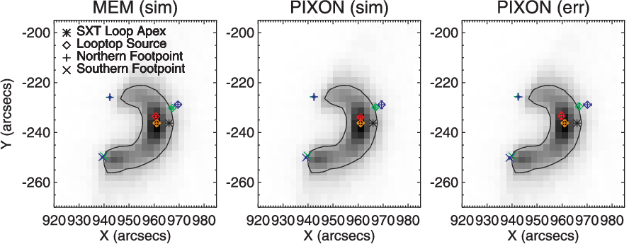
Further comparisons are made quantitatively. In a similar approach taken by Aschwanden et al. [4], we measure the centroid position of the loop-top source, and compute its height, in each HXT energy band (except the H-band), with respect to the conjugate footpoints in the M1-band. For SXT, following Aschwanden et al. [4], the brightness maximum at the enhanced loop top is pinpointed, for which the measurement error is estimated to be half of the SXT CCD pixel size (, or 1750 km). To compare with the result given by Masuda et al. [17] that the M1-band coronal source was above the apex of the SXT loop by 7000 km, we draw a line connecting the midpoint of the M1-band footpoints and the brightness maximum of the SXT loop, and choose the pixel where the line intersects the SXT 30% brightness contour (see 3) as a conservative proxy for the loop apex.
To estimate the uncertainties of the hard X-ray source locations, we simulate the HXT images by adding random noise to the data counts collected by each of the 64 subcollimators, , i.e.,
where is a pseudo-random number generated by the IDL procedure RANDOMN. A new image can be reconstructed based on and the source centroids are measured. In practice, a box is specified to enclose each individual source in an image. A region is allowed to grow from the local maximum inside each box to include all connected neighbors whose values are above a given minimum (see the REGION_GROW function in IDL), which is chosen interactively so that the region takes the shape of an ellipse. The centroid position is determined by fitting a 2D elliptical Gaussian equation to each individual region. By repeating the above procedure for many times (30 times in our work), we get a distribution of the source centroids, and their uncertainties can be approximated by standard deviation. The flux uncertainty of each individual source as shown in 2 can also be obtained from the simulated images (see Table 1) by integrating the flux inside a box region containing the source.
For the Pixon algorithm, alternatively, an error map (1- error at each pixel) can be obtained for the reconstructed image. Thus, we can estimate the uncertainties of the source centroids by adding (substracting) the error map to (from) the reconstructed Pixon map, getting the “new” source locations, and then comparing with those obtained from the Pixon map alone. The larger of the differences is taken as the error bar.
In 3, we show the source centroids during the fast rise phase (17:27:35–17:28:15 UT), with corresponding error bars estimated from simulated MEM (left panel) and Pixon (middle panel) images, as well as from Pixon error maps (right panel). Sources in different HXT energy bands are represented with the same color code as in 1. The brightness maximum of the SXT loop top is shown in orange, and its apex is denoted by an asterisk. One can see that the accuracy of the HXT loop-top centroid position is comparable to that of the brightest SXT pixel, despite that the FWHM of the finest HXT collimator is as large as 6000 km. The footpoint positions are even more accurate, with sub-arcsec precision being achieved.
Various geometrical parameters can then be derived and their error bars are computed following the rules of the propagation of uncertainty44 4 A note of caveat should be made that the SXT–HXT co-alignment error is not included. However, it is generally better than [16], less than the error of locating the brightest SXT pixel (900 km).. The results are listed in Table 2. For comparison, corresponding numbers given by Aschwanden et al. [4] and Masuda et al. [17] are also listed in bold and slanted face, respectively. One obvious difference is the smaller separation of M1-band coronal source from the brightness maximum of the SXT loop. The height difference, in Table 2 ( km in Pixon and km in MEM), is almost half of that measured by Aschwanden et al. [4, 9600 km]. The height difference between the M1-band coronal source and the apex of the SXT loop, in Table 2 ( km in Pixon and km in MEM), is also much smaller than that given by Masuda et al. [17, 7000km]. The new measurement is in agreement with RHESSI observations [13] that typical impulsive phase coronal emission is only slightly above the thermal loop (), which, however, is measured by the radial difference of the center of mass locations. This is slightly different from the approach taken by Aschwanden et al. [4] and this paper.
Accordingly, the M1-band coronal source is also less separated from the L-band loop top in terms of centroid positions. Thus, any reasonably chosen integration region containing the M1-band source in imaging spectroscopic analysis will inevitably include much more L-band photon counts than it would with the original HXT images, therefore leading to a much larger L- and M1-band ratio, as we shall demonstrate in Section 3.
III Spectroscopy
III.1 Historical Investigations and Interpretations
| Time Interval (UT) | Algorithm | TCS (MK) | |||||
|---|---|---|---|---|---|---|---|
| L/M1 | M1/M2 | L/M1 | M1/M2 | L/M1 | M1/M2 | ||
| 17:26:52–17:27:3911From Masuda et al. [17], Masuda et al. [16] | MEM | 2.6 | 4.1 | 200 | 130 | ||
| 17:27:40–17:28:2022From Alexander & Metcalf [1] and Metcalf & Alexander [19] | Pixon | 2.20.6 | 4.10.2 | 3.30.1 | 3.50.1 | 215 | 120 |
| 17:27:35–17:28:1533From Masuda et al. [18] | MEM | 4.0 | 5.5 | 3.2 | 3.8 | 100 | 90 |
| 44From Petrosian et al. [22], who specified only a time instant, 17:28:04 UT, but not the time interval for data accumulation. Note also that is derived for each individual footpoint. | MEM | 4.2 | 6.8 | 3.1/2.5 | 3.9/3.7 | ||
Limited spectral information from HXT images can be derived by calculating flux ratios between adjacent energy bands. We denote the photon spectral index derived from L- and M1-band as , and that from M1- and M2-band as , with the superscripts, CS and FP, standing for the coronal source and the footpoints, respectively. Corresponding electron indices are denoted by in a usual fashion. From Table 3, one can see that the coronal spectrum is considerably softer in the post-calibration era [18, 22] than in the pre-calibration era [17, 16, 1, 19]. Different decisions made by data analyzers in the same era, e.g., different integration region and time interval for data accumulation, appear to result in only minimal differences, however.
In the pre-calibration era, the verdict for the Masuda flare is that the coronal emission was nonthermal [1, e.g.,]. The thermal interpretation [17, e.g.,] was largely rejected due to the following three major arguments: (a) the thermal bremsstrahlung requires an extremely hot plasma (up to MK), for which there was no evidence from other instruments, e.g. the impulsive phase BCS Fe XXV spectra, assumed from the loop top, give a source temperature of MK [9]; (b) the temperature derived from the HXT lower channels is much higher ( MK) than that from the higher channels [1, 12515 MK;]; and (c) the time variability of the coronal source was too rapid (similar to that of the footpoints) to be consistent with thermal cooling times [11]. We will check these arguments against the re-calibrated data in §4.2.
On the other hand, it is very difficult to understand the extremely hard spectrum of the coronal source, which had a power-law index of 2 from the L- and M1-band ratio. Though it may indicate a possible turnover in a nonthermal electron spectrum, such a flat spectral index is close to the hardest theoretically possible bremsstrahlung spectrum. Nevertheless, putting in the perspective of the thick-thin target model [31], which argues that a coronal source acts as a thick target () for electrons at lower energies and thin target () for higher energies, one can derive that the spectral index of the injecting electrons for the coronal source, , while that for the footpoint emission, . Note, however, that the thick-thin target model assumes that the same electron population is responsible for both the coronal and the footpoint emission. A promising explanation is electron trapping in the corona, with energy losses dominated by collisions [1]. Since the collisional deflection time of an electron of energy ,
where is the electron density and the Coulomb logarithm ( under solar conditions), the longer life time of more energetic electrons would result in the erosion of the low-energy regime of the velocity distribution function, therefore the progressive spectral hardening, on timescales in the order of 10–100 s for a coronal density of order cm-3.
The coronal trapping of energetic electrons predicts that the injecting spectrum for the coronal source is hardening for 1.5 powers relative to the corresponding footpoint emission in the weak diffusion limit (see §4.3). It also leads to the progressive delay of hard X-ray peaks with increasing energy, due to collisional precipitation of the trapped electrons [5, e.g.,]. Based on time-of-flight measurements, Aschwanden et al. [5] found 5 hard X-ray coronal sources that can be explained by a coronal trap in the weak diffusion limit. The same 5 events were also studied by Metcalf & Alexander [19], who were looking for the spectral evidence of trapping. Two of them, including the Masuda flare, were found to be consistent with impulsive phase coronal trapping in the thick-thin target scenario.
In the post-calibration era, in contrast, the spectrum of the Masuda loop-top source looks rather soft [18, 22], with its spectral indices falling in the typical range of recent RHESSI observations [13, 4–7;]. Using the MEM algorithm, Masuda et al. [18] reported that the loop-top spectrum can be well fit by emission from an isothermal plasma of about 100 MK. In §3.2, we present a re-analysis of the Masuda flare with both MEM and Pixon algorithms, and in Section 4, discuss the implications of the changes introduced by the re-calibration.
III.2 Re-Analysis
| Time Interval (UT) | Algorithm | (MK) | 11Spectral indices derived from single power law fits of the corresponding Yohkoh Wide Band Spectrometer (WBS) spectra. | ||||||
|---|---|---|---|---|---|---|---|---|---|
| L/M1 | M1/M2 | L/M1 | M1/M2 | L/M1 | M1/M2 | L/M1/M2 | |||
| 17:26:50–17:27:35 | MEM | 4.50.7 | 5.31.3 | 3.30.4 | 4.60.5 | 4.03 | |||
| Pixon | 4.60.3 | 5.00.4 | 3.20.3 | 4.00.2 | |||||
| 17:27:35–17:28:1522Integration regions are specified in 4. | MEM | 4.50.4 | 5.91.1 | 2.50.2 | 3.70.2 | 3.69 | |||
| Pixon | 4.70.2 | 5.80.5 | 1.90.2 | 3.30.1 | |||||
| 17:28:15–17:29:00 | MEM | 5.80.7 | 5.61.8 | 1.80.2 | 3.50.1 | 3.36 | |||
| Pixon | 6.60.4 | 10.05.1 | 1.30.5 | 3.10.1 | |||||

| Time Interval (UT) | Algorithm | (MK) | ||||||
|---|---|---|---|---|---|---|---|---|
| L/M1 | M1/M2 | L/M1 | M1/M2 | L/M1 | M1/M2 | L/M1/M2 | ||
| 17:26:50–17:27:35 | MEM | 4.30.8 | 4.81.4 | 3.30.4 | 4.60.5 | |||
| Pixon | 4.40.3 | 4.80.4 | 3.20.3 | 4.00.2 | ||||
| 17:27:35–17:28:1511Integration regions are specified in 5. | MEM | 3.00.7 | 5.41.3 | 2.30.2 | 3.60.2 | |||
| Pixon | 3.40.5 | 5.10.5 | 1.80.2 | 3.30.1 | ||||

The region growing method (see Section 2) is also used to specify the integration region for each individual hard X-ray source in imaging spectroscopic analysis. This is a convenient method to “extract” weak sources, and the same integration region can be recovered as long as the same minimum threshold is specified. Integration regions chosen for the fast rise phase of the flare are specified as an example in Figures 4 and 5. In 4 the integration regions cover emission from both the M1- and M2-band, and the corresponding results are listed in Table 4; in 5, integration is carried out over the regions with significant M2-band emission only, and the corresponding results are listed in Table 5. Table 5 does not include the decay phase, during which there is no visible M2-band coronal emission. From both tables, one can see that our results are basically in agreement with Masuda et al. [18] and Petrosian et al. [22]. In addition, one can see that the photon spectra of the footpoint emission are hardening throughout the hard X-ray burst. In contrast, the spectra of the coronal emission are successively softening, which we shall discuss in §4.3.
IV Discussion and Conclusion
IV.1 Impact of the Geometrical Change
There are three major difficulties in understanding the original Masuda flare, viz., 1) the lack of L-band emission at the coronal source and consequently the extremely flat spectrum of the coronal source below 20 keV [17, 1]; 2) the apparently low density at the location of the coronal source due to the lack of SXT emission; and 3) the lack of soft X-ray signature of hydrodynamic response at the presumed field lines that connected the hard X-ray coronal source to the chromosphere [1]. Also, the soft X-ray loop barely grows with time, defying the theory of choromospheric evaporation. All three difficulties can be arguably attributed to the elevated hard X-ray coronal source in the original data. Thus, the reduction of the source height relative to the soft X-ray loop in the re-calibrated data has more or less relieved these difficulties.
We will discuss the 3rd difficulty in §4.3. As for the first one, although the spectrum has become softer at lower energies with the re-calibrated data, the fact that the Masuda source is poorly imaged in the L-band remains a puzzle. It might be due to a turnover in non-thermal electron spectrum, or to instrumental effects, or simply to the poor resolution of HXT. In any case, the L- and M1-band ratio reflects poorly the true spectral slope.
The 2nd point deserves some further comments. The column depth required to stop electrons at 20 keV, the approximate break energy of the coronal spectrum, is cm-2, which can be estimated from the formula [31, e.g.,]
where is in erg, N is in cm-2, and , with the electron charge ( esu). Given a source length of cm, the density, , is as large as cm-3. This, however, agrees approximately with Aschwanden et al. [3] who found the electron density in the flare trap of the Masuda flare, cm-3, by fitting the hard X-ray energy-dependent time delays with the electron collisional deflection time. The trap density is lower than the peak density in the SXT loop top, cm-3[3], but at least an order of magnitude larger than the density at the original coronal source location, e.g., cm-3, inferred from HXT data by Masuda et al. [17], or cm-3, inferred from both HXT and SXT data by Tsuneta et al. [28]. Hence the coronal trap must be located above the brightness maximum of the SXT loop, but lower in altitude than the original Masuda source. If the trap location is consistent with the current source location, the condition for the confinement of nonthermal electrons at the loop-top region is much less stringent than that imposed by the original data. For example, a 20 keV electron needs to bounce only 5 times for the thick target hypothesis to be effective, in contrast to more than 30 times of bounce as required by the original data, given the column depth, cm-2 [28].
In view of the argument above, the thick-thin target model proposed by Wheatland & Melrose [31] looks quite promising. It is noteworthy that the SXT loop is clearly visible at the flare onset (the bottom panel of 1), suggesting that the coronal atmosphere has already been heated to a dense and hot state prior to impulsive electron acceleration. If the corona is dense enough, it can stop the less energetic electrons to produce a bright, thick-target coronal source in the L-band, and a much dimmer, thin-target one in higher-energy bands. RHESSI has observed coronal sources brighter than footpoints at energies up to 50 keV [29], which take the shape of a loop and are explained by the thick-target model. We will test the re-calibrated data against the thick-thin target model (§4.3), but before that we first re-examine the thermal interpretation (§4.2).
IV.2 Thermal Interpretation
From Table 4, one can see that a consistent temperature can be derived from two different HXT channel ratios (L/M1 and M1/M2), in contrast to previous publications [17, 1]. In Table 5, temperatures derived from the lower HXT channel ratio are indeed higher than those from the higher channel ratio during the fast rise phase, probably suggesting the existence of a nonthermal component, despite that the two temperatures still fall within the same error range.
We now check another major argument against the thermal interpretation, viz., the time variability of the coronal source is much shorter than the electron thermalization time for Coulomb collisions [11],
With cm-3 (assuming a unity filling factor) and MK from Masuda et al. [17], s. This number has been commonly cited in the literature, out of the context of specific plasma parameters. With cm-3 estimated by Tsuneta et al. [28] and MK from our analysis, however, is about 1.4 s. If the trap density ( cm-3) inferred by Aschwanden et al. [3] is adopted, could be as small as 0.2 s. Thus, the thermal interpretation cannot be ruled out unambiguously, based on the spectral information available. However, the temperature is still much higher than that derived from BCS Fe XXV spectra [9, MK;]. Moreover, a single thermal fit can be excluded for most hard X-ray coronal sources observed by RHESSI [13]. These observations cast doubt on the thermal interpretation of the Masuda flare.
IV.3 Thick-Thin Target and Trapping

Following the thick-thin target model [31], we assume that the coronal source acts as a thick target for less energetic electrons (), and a thin target for more energetic electrons (). With low-energy electrons stopped in the loop-top region, the footpoint emission is not supposed to follow power laws at low energies, but a thick target is assumed at high energies as usual (). The derived electron indices are given in Table 6, in which we only use the photon indices obtained by Pixon. One should trust more than , since the latter is inevitably contaminated by thermal emission, especially for the integration region that covers both the M1- and M2-band emission. The thick-thin target model agrees well with the observation during the fast rise phase of the hard X-ray burst, when , , and are approximately equal to each other (shown in bold face in Table 6). During the slow rise phase, however, is significantly smaller than .
One difficulty in understanding the Masuda flare (see §4.1) lies in the lack of signature of choromospheric evaporation. This can be understood if the less energetic electrons, which constitute the bulk energy of injecting electrons, are mostly stopped in the dense corona, as indicated by the existence of the soft X-ray loop at the flare onset (1). In that case, chromospheric evaporation would be strongly suppressed, due not only to reduced energy deposited in the chromosphere, but also to enhanced inertia of the overlying material [8]. Moreover, the fact that the electrons interact with hot coronal plasma rather than a “cold target” reduces the energy-loss rate, hence fewer electrons are required at low energies, which helps to alleviate the electron number problem [7].
| Time Interval (UT) | Integration Region | |||
|---|---|---|---|---|
| 17:26:50–17:27:35 | M1 & M2 | 5.6 | 4.00.4 | 5.00.2 |
| M2 | 5.40.3 | 3.80.4 | 5.00.2 | |
| 17:27:35–17:28:15 | M1 & M2 | 5.70.2 | 4.80.5 | 4.30.1 |
| M2 | 4.40.5 | 4.10.5 | 4.30.1 |
The spectral characteristics revealed in Table 6 seem to put the coronal trap in the weak pitch angle diffusion regime, in which the loss cone is empty, while the opposite case, that the loss cone is filled with scattered particles, is defined as the strong diffusion. Specifically, in a trap-and-precipitation scenario, the precipitation rate, , can be evaluated as,
where is the loss-cone angle. If the data accumulation time is significantly longer than the trapping time (), which is often the case, the observed injecting electron spectrum for the coronal source in relation to that for the corresponding footpoint emission would satisfy the following inequality [19, c.f., the Appendix in],
with the lower (higher) bound corresponding to the weak (strong) diffusion limit.
The decrease in the additional hardening of relative to with time, as indicated in Table 6, may suggest an enhanced scattering rate. Alternatively, this can be attributed to an interesting effect in the standard flare model, namely, field line shrinkage [10, e.g.,]. The cartoon in 6 shows that the magnetic field strength at the soft X-ray loop top would increase with time, as the newly reconnected, cusp-shaped field lines “shrink” and relax into a more potential state, piling up above the soft X-ray loop. As we know, the loss-cone angle, , is defined through the formula,
where and are the magnetic field strength at the footpoint and at the coronal trap, respectively. The increase of the magnetic field strength at the coronal trap would result in the enlargement of the loss cone, and therefore the enhancement of the precipitation rate, if we assume that electrons are continuously injecting into the trap. Electrons that are trapped before the field line shrinkage, however, would not be affected by the strengthening , as their perpendicular momenta also increase due to the conservation of the transversal adiabatic invariant, .
With the depletion of energetic electrons, the hard X-ray coronal emission would become weaker relative to the footpoints. Its centroid location would move to a slightly higher altitude relative to the soft X-ray loop, because electrons trapped at lower magnetic loops (with larger loss-cone angles) would be depleted from the coronal trap first. With the enhanced precipitation rate, low-energy electrons would still be stopped at the thick-thin target, but more high-energy electrons would precipitate towards the chromosphere. Thus, the footpoint spectrum would be successively hardening, while the coronal spectrum successive softening, as observed in the Masuda flare.
To summarize, we demonstrate through an uncertainty analysis that the hard X-ray coronal source of the Masuda flare is located much closer to the soft X-ray loop in the re-calibrated HXT images than in the original ones. This may account for the change of the spectral characteristics of the coronal source derived from imaging spectroscopic analysis.
References
- [1] Alexander, D. & Metcalf, T. R. 1997, ApJ, 489, 442
- [2] Aschwanden, M. J. 2002, Space Sci. Rev., 101, 1
- [3] Aschwanden, M. J., Bynum, R. M., Kosugi, T., Hudson, H. S., & Schwartz, R. A. 1997, ApJ, 487, 936
- [4] Aschwanden, M. J., Hudson, H., Kosugi, T., & Schwartz, R. A. 1996a, ApJ, 464, 985
- [5] Aschwanden, M. J., Kosugi, T., Hudson, H. S., Wills, M. J., & Schwartz, R. A. 1996b, ApJ, 470, 1198
- [6] Battaglia, M. & Benz, A. O. 2007, A&A, 466, 713
- [7] Emslie, A. G. 2003, ApJ, 595, L119
- [8] Emslie, A. G., Li, P., & Mariska, J. T. 1992, ApJ, 399, 714
- [9] Fletcher, L. 1999, in ESA Special Publication, Vol. 448, Magnetic Fields and Solar Processes, ed. A. Wilson & et al., 693–700
- [10] Forbes, T. G. & Acton, L. W. 1996, ApJ, 459, 330
- [11] Hudson, H. & Ryan, J. 1995, ARA&A, 33, 239
- [12] Krucker, S., Battaglia, M., Cargill, P. J., et al. 2008, A&A Rev., 16, 155
- [13] Krucker, S. & Lin, R. P. 2008, ApJ, 673, 1181
- [14] Li, Y. P. & Gan, W. Q. 2007, Advances in Space Research, 39, 1389
- [15] Liu, W., Petrosian, V., Dennis, B. R., & Jiang, Y. W. 2008, ApJ, 676, 704
- [16] Masuda, S., Kosugi, T., Hara, H., Sakao, T., Shibata, K., & Tsuneta, S. 1995, PASJ, 47, 677
- [17] Masuda, S., Kosugi, T., Hara, H., Tsuneta, S., & Ogawara, Y. 1994, Nature, 371, 495
- [18] Masuda, S., Sato, J., Kosugi, T., & Sakao, T. 2000, Adv. Space Res., 26, 493
- [19] Metcalf, T. R. & Alexander, D. 1999, ApJ, 522, 1108
- [20] Metcalf, T. R., Hudson, H. S., Kosugi, T., et al. 1996, ApJ, 466, 585
- [21] Ogawara, Y., Takano, T., Kato, T., et al. 1991, Sol. Phys., 136, 1
- [22] Petrosian, V., Donaghy, T. Q., & McTiernan, J. M. 2002, ApJ, 569, 459
- [23] Pick, M., Démoulin, P., Krucker, S., Malandraki, O., & Maia, D. 2005, ApJ, 625, 1019
- [24] Sato, J., Kosugi, T., & Makishima, K. 1999, PASJ, 51, 127
- [25] Sui, L. & Holman, G. D. 2003, ApJ, 596, L251
- [26] Sui, L., Holman, G. D., & Dennis, B. R. 2004, ApJ, 612, 546
- [27] Tomczak, M. 2001, A&A, 366, 294
- [28] Tsuneta, S., Masuda, S., Kosugi, T., & Sato, J. 1997, ApJ, 478, 787
- [29] Veronig, A. M. & Brown, J. C. 2004, ApJ, 603, L117
- [30] Veronig, A. M., Karlický, M., Vršnak, B., et al. 2006, A&A, 446, 675
- [31] Wheatland, M. S. & Melrose, D. B. 1995, Sol. Phys., 158, 283