Analytically Solvable Asymptotic Model of Atrial Excitability
Abstract
We report a three-variable simplified model of excitation fronts in human
atrial tissue. The model is derived by novel asymptotic techniques
from the biophysically realistic model of Courtemanche et al.
[11] in extension of our previous similar models.
An iterative analytical solution of the model is presented
which is in excellent quantitative agreement with the realistic
model.
It opens new possibilities for analytical studies as well as for
efficient numerical simulation of this and other cardiac models of
similar structure.
Published in ”Mathematical Modeling of Biological Systems” ,
Vol 2, A. Deutsch, R. Bravo de la Parra, R. de Boer et al. (eds.)
Birkhaeuser, Boston, pp. 289-302, DOI:10.1007/978-0-8176-4556-4_26,
2008.
Keywords:
cardiac modelling, asymptotics, excitation, wave front0.1 Introduction
The mechanical activity of the heart is controlled by electrical impulses propagating regularly through it during our entire lifespans [22]. A disturbance in the regular propagation may lead to life-threatening cardiac arrhythmias [31]. Sudden cardiac death, for instance, accounts for 300 000 to 400 000 deaths annually in the United States alone [14, 23], i.e. more than AIDS, breast and lung cancer. This entails intensive research into the mechanisms of heart functioning and failure. The accumulated information reveals an overwhelming complexity of the patterns of electrical cardiac activity.
True understanding of the experimental data requires the development of appropriate qualitative cardiac models [10, 19, 20]. One approach to cardiac modelling is to take into account the various levels of membrane, cellular and myocardial structure and their interactions and to model the action potential (AP) on the basis of experimental measurements of ion fluxes in as much detail as possible. The resulting models are known as realistic or detailed ionic models. The first example of this type of models was developed by Noble [25, 26] and there are now such models for various cardiac cells in different species, e.g. [3, 12, 21, 27, 35] and many others. However, since these models are very complex and highly nonlinear, it is difficult to assess contribution of specific model components to different patterns of activity. Furthermore, their computation is arduous because they contain a large number of equations and small parameters. They become very expensive and time-consuming especially when large volumes of tissue are simulated. One possible alternative is to search for simplified models which could mimic the most important AP properties, allow analytical studies and reduce the computing requirements. Many simplified models have been suggested, either phenomenologically, or based on the structure of the realistic models, [1, 4, 13, 15, 18] etc.. However, all of these models contain arbitrary elements in the sense that they are not derived from any of the realistic biophysical cell models and lack explicit correspondence with the biophysical structure of the cardiac tissues. E.g. van der Pol and van der Mark modelled heartbeat as an electronic relaxation oscillator[28].
Our recent studies [8, 32, 33, 7] have demonstrated a serious disadvantage of the most popular and successful simplified generic model of cardiac excitability – the FitzHugh-Nagumo (FHN) equations [17, 24]. It cannot describe adequately the one feature of excitation propagation which is most important for medical applications, namely the way regular propagation fails and arrhythmias occur. An excitation wave in real atrial tissue, or in a realistic model, may fail to propagate if the temporal gradient of the transmembrane voltage at the front becomes too small to excite the tissue ahead of it e.g. if the wave fails to propagate fast enough [8]. Then the wave front looses its sharp spatial gradient and its further spread is purely diffusive, i.e. the front dissipates. This happens long before the back of the excitation impulse catches up with the front. This type of propagation failure does not exist in a FitzHugh-Nagumo type model [6] since it is known that the propagation of a wave front in this system may be slowed down, halted or even reversed [16]. This phenomenon is illustrated in figure 1: a temporary block of excitability only temporary halts the FHN wave, but completely disrupts propagation in the realistic model, even though it lasts much shorter than the AP.

Earlier we have proposed novel asymptotic methods of reduction of cardiac equations [9]. In this paper we use these methods to derive a three-component description of the propagating excitation fronts and their dissipation. The virtue of our model is that it reproduces propagation failure unlike the FitzHugh-Nagumo models because it is derived in a reliable way from the realistic ionic model. We also report an analytical solution for this three-component model. The analytical solution is constructed as an iterative procedure and it may be seen as a generalisation in which the caricature solutions presented in our earlier papers [5, 6, 30] appear as first approximations. This, is to our knowledge, the first analytical solution, albeit in quadratures, which gives a numerically accurate prediction of the front propagation velocity (within 16%) and its profile (within 0.7 mV) in human atrial tissue.
0.2 Mathematical formulation of the problem
Atrial tissue model. In our study atrial tissue is a one-dimensional, homogeneous and isotropic medium satisfying a system of reaction–diffusion equations
| (1) |
where is a vector defined according to the atrial single-cell realistic CRN model [11], is the vector of all dynamic variables of the model and is the tensor of diffusion in which only the coefficient of the voltage is nonzero. This simplified description focuses on the excitation and propagation of impulses, while ignoring the effects due to geometry, anisotropy and heterogeneity of a real atrium.
Asymptotic reduction. In order to reduce the dimension and complexity of the problem, we perform a formal analysis of the time scales of dynamic variables. For the system (1) we define characteristic time scale functions, and compare their magnitudes obtained numerically for a space-clamped version of the system as shown in figure 2. The variables, whose time scales are relatively small, are fast variables since they change significantly during the upstroke of a typical AP, while all other variables, whose time scales are relatively large, are slow variables because they change only slightly during this period. Figure 2(a) demonstrates that the variables , , , , , , are fast variables comparable with the time scale of the AP upstroke.


A specific feature of system (1) is that of the various ionic currents in the system only the sodium current is significantly large during the AP upstroke, whereas other currents are small at this stage as can be seen in figure 2(d). Secondly, the fast sodium current is only large during the AP upstroke, and almost vanishes otherwise, because either gate or gate or both are nearly closed outside the upstroke since their quasistationary values and are small there as illustrated in figure 2(b).
To formalise the distinction between fast and slow terms we perform an asymptotic embedding of system (1). We introduce an artificial parameter into the system so that for the original system is recovered, while in the limit only the terms comparable with the time scale of the AP upstroke are retained,
| (6) |
where is the Heaviside function, is the sum of all currents except the fast sodium current , the dynamic variables , , , , and are defined in [11], is the vector of all other, slower variables, and is the vector of the corresponding right-hand sides. Novel features of the asymptotic embedding (6), non-standard in comparison with the theory of fast-slow systems [34, 29, 2] are (a) the introduction of the asymptotic factor only at one term in the right-hand side of the equation for whereas the standard factor at the derivative would be equivalent to factor at the whole right-hand side, and (b) that in the limit , functions and have to be considered zero in certain overlapping intervals and , and , hence the representations and . These aspects, as applied to the fast sodium current, have been shown to be crucial for the correct description of the propagation block [5]. A more detailed discussion of the parameterisation (6) can be found in reference [9].
The exact value of is not essential for the theoretical analysis, as its change is equivalent to rescaling of the spatial coordinate. To operate with dimensional velocity, we assume the values , as in [8, 9] and F cm-1. We perform the scaling , , take the limit and notice that the equations for the variables denoted by in (6) decouple from the voltage equation. Thus we arrive at the conclusion that only the following three-variable system needs to be considered for a description of the propagation of an AP front or its failure,
| (7a) | ||||
| (7b) | ||||
| (7c) | ||||
In other words, we consider the fast time scale on which the upstroke of the AP occurs, neglect the variations of slow variables during this period as well as all transmembrane currents except , as they do not make significant contribution during this period and replace and with zero when they are small. The parameters and functions in (7) are defined as in [11], namely
| (8a) | ||||
| (8b) | ||||
Two new ‘gate threshold’ parameters and appear in the system and are chosen from the conditions and . As follows from the derivation, variable , the slow inactivation gate of the fast sodium current, acts as a parameter of the model. It is the only one of all slow variables included in the vector that affects our fast subsystem. We say that it describes the excitability of the tissue.
Travelling waves and reduction to ODE. We look for solutions in the form of a front propagating with a constant speed and shape. So we use the ansatz for where is the dimensionless wave speed of the front, related to the dimensional speed by . Then equations (7) reduce to
| (9a) | ||||
| (9b) | ||||
| (9c) | ||||
where the boundary conditions are given by
| (10a) | ||||||||
| (10b) | ||||||||
Here and are the pre- and post-front voltages, and .
Equations (9) represent a system of fourth order so its general solution depends on four arbitrary constants. Together with constants , and this makes seven constants to be determined from the six boundary conditions in (10). Thus, we should have a one-parameter family of solutions, i.e. one of the parameters can be chosen arbitrary from a certain range.
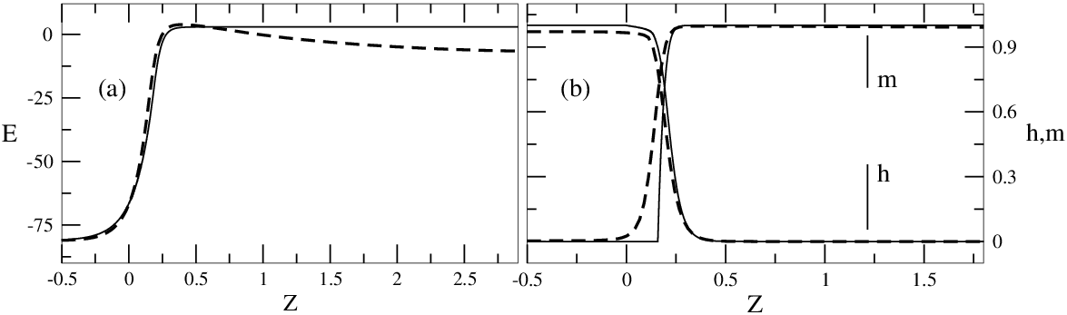
Comparison of the three-variable model (9) with the realistic CRN model [11]. The simplified three-variable model (7) and its ODE version (9) provide an excellent approximation to the fronts of the action potential in human atrial tissue as demonstrated in figure 3 where a comparison with the solution of the realistic CRN model [11] is presented. As must be expected the voltage in the simplified model remains constant after reaching its post-front value while the voltage in the CRN model assumes a shape typical for an action potential. To quantify further the comparison between the two models below we list the values of the wave speed, the post-front voltage and the maximum rate of AP rise. For the realistic model [11] these values are mm/ms, mV and V/s. The respective values for the simplified model (9) are mm/ms, mV and V/s. The relative errors made by the simplified model in estimating the wave speed and the the maximum rate of AP rise are 16% and 11%, respectively, and the absolute error in estimating the post-front voltage is mV.
We recall that our main motivation for the derivation of the three-variable simplified model was to reproduce the realistic front dissipation behaviour of atrial tissue as it appears for example in the CRN model [11]. The third column of figure 1 illustrates the dissipation of a propagating front in equations (7) in response to a temporary block of excitability. It is observed that the dissipation behaviour of the simplified system resembles the one of the realistic CRN model In this aspect of the behaviour our model is superior to the simplified models of FitzHugh-Nagumo type.
0.3 Iterative analytical solution
Exact solution for . For the reduced model (9),(10a) has a two-parameter family of exact solutions, with parameters and . Since the boundary condition is an equilibrium point of (9c), remains a solution for all . It follows that (9a) is a constant-coefficient linear homogeneous equation in this interval, and its solution
| (11) |
satisfies boundary conditions , and , provided that the internal boundary point is located at
| (12) |
Finally, is a solution of (9b) with boundary condition in the interval , because it belongs to its equilibrium set. In the interval , (9b) can be re-written in the form
| (13) |
and its solution can be immediately obtained,
| (14) |
Approximate solutions for . For , we rewrite (9) as
| (15a) | ||||
| (15b) | ||||
| (15c) | ||||
where
| (16) |
The boundary conditions are
| (17a) | ||||
| (17b) | ||||
| (17c) | ||||
| (17d) | ||||
| (17e) | ||||
This problem is equivalent to the following system of integral equations
| (18a) | ||||
| (18b) | ||||
| (18c) | ||||
| (18d) | ||||
The last equation Eq. 18d imposes an additional relationship between parameters and , so the ultimate solution depends only on one arbitrary parameter, say , which in reality may be determined by the pre-history of the medium through which the excitation front propagates.
The system Eq. 10 can be solved by iterations, starting from a suitable initial approximation. The iterations converge for a number of various initial approximations, see figure 4. In section 0.4 we discuss two selected initial approximations. The first of them, A1, is favourable from a numerical point of view. The second one, A2, is important in the context of our recent work [30] since it leads to an even further formal simplification of problem (9) to a system which allows exact solution and extensive analytical study.
0.4 Selected initial approximations
A1: The small-diffusion initial approximation. A simple initial approximation may be obtained by considering a space-clamped version of (9) corresponding to the limit of very small constant of diffusion in equations (6) (note that this is applied only to the solution in the interval ) and replacing the gating variable with its quasi-stationary value which in our asymptotic limit and for equals 1. Hence, an initial approximation may be chosen to satisfy
| (19a) | ||||
| (19b) | ||||
This system can be solved in quadratures,
| (20a) | ||||
| (20b) | ||||
where the initial conditions and are given by Eq. 17a and Eq. 17c.
A2: The ‘caricature’ initial approximation. An even simpler initial approximation is
| (21) |
In this case functions of voltage , and take constant values , and , respectively. Then quadratures (18) for the results of the first iteration are obtained in explicit formulae; moreover, (18d) is resolved explicitly. These explicit formulae have been reported in our recent work [30] (see formulae (9) of that paper). There this piecewise-linear simplification was considered only as an arbitrary “caricature” with the purpose of merely analysing qualitative features of the solution set. Here we note that it actually appears naturally as a step the iterative procedure leading to a numerically accurate solution.
The iterative analytical solution (18) obtained from these initial approximations, is indistinguishable from the numerical solution of (9) after some 30 iterations and has the shape of a travelling front as shown in figure 3.

Convergence and uniqueness of the iterative solution (18). The iteration procedure produced by (18) is nonlinear and non-monotonic, and we do not have a rigorous proof of its convergence from any given initial approximation. Likewise, we do not have a rigorous proof that the solution of the boundary-value problem (17) is unique. However it is straightforward to see that if the iterations converge, the result is a solution of the boundary value problem, due to the above mentioned equivalence of (17) and the system of integral equations (18). Figure 4 illustrates that the first several iterations obtained from different initial approximations oscillate about the correct numerical solution of the problem and ultimately converge to it. The “small diffusion” initial approximation A1 is particularly interesting because the results of the second iteration are already very close to the accurate numerical values for the wave speed and the post-front voltage. Indeed, if the excitability parameter and the pre-front voltage are chosen at their physiological resting values and mV, respectively [11], at the second step of the iterations the value of the dimensional wave speed is mm/ms which has only 20% relative error compared to the value mm/ms of the realistic ionic model (0.2) and 5% relative error compared to the value mm/ms obtained numerically from equations (9). Similarly the post-front voltage mV compares well with the value 3.36 mV of the CRN model (0.2). Clearly, the second iteration obtained from initial approximation A1 introduces certain errors. Numerically, however, it is immensely superior to any other numerical scheme because it involves only a single evaluation of formulae (20) and a two-fold evaluation of formulae (18). In addition, the dangers of numerical divergence associated with many of the alternative numerical schemes for solving problems (0.2) or (9) are avoided since the above expressions are mathematically well-behaved.
The two initial approximations discussed above are essentially different. In the small-diffusion approximation the initial guess for the voltage is a function while in the ‘caricature’ approximation it is a constant const. The fact that two essentially different initial approximations give the same limits is a strong indication that the iterative procedure leads to a unique solution. To support this claim further we have performed calculations starting from initial approximation A2 with initial values . In all cases the iterations converged to the same solution, in a similar manner to those shown on figure 4. The small-diffusion initial approximation is not discussed here because its initial guess is the unique solution (20) of equations (19) and thus it does not depend on any arbitrary parameters.
So, although we cannot exclude the possibility that the iteration procedure may not converge from some “bad” initial guess, the examples considered provide an evidence that a reasonable initial approximation always gives converging iterations, and the solution is unique.
0.5 Discussion
We have presented an analytical approach to the description of the speed and the structure of an excitation front in a model of human atrial tissue [11]. We have identified small parameters in the realistic model and used asymptotic arguments to obtain a simplified three-variable model of the excitation front. Although we have explicitly used certain quantitative features of atrial tissue [11], the main properties used are generic for cardiac excitation models so the approach should be applicable, possibly with suitable modifications, to other cardiac equations models too. Our model takes the form of a nonlinear eigenvalue problem with a piece-wise right-hand side defined over three voltage intervals. This model is solved explicitly in the first two intervals, and in the last interval we have suggested an analytical iterative procedure capable of producing a solution with a good accuracy already after the first iteration. The iterative procedure can be started from reasonably chosen simple initial approximations and converges to a unique solution which differs only within few percent from the solution of the realistic ionic atrial model.
An important feature of our approach is that it is capable of correctly describing the excitation propagation at reduced excitabilities, up to a complete block of propagation via “front dissipation” mechanism, which is completely unachievable by traditional analytical approaches based on FitzHugh-Nagumo type of equations. This aspect has been analysed in our earlier publications [5, 6, 9, 30]. In particular, our recent study [30] is devoted to a discussion of one practical application of our approach. There we have used a numerical solution of the simplified three-variable model (9) to propose a simple criterion for break-up and self-termination of spiralling waves and have confirmed our predictions by numerical simulations of the realistic model of Courtemanche et al.. However, the important question of finding an analytical solution of our simplified model (9) was now solved in this paper.
The possibility of obtaining numerically reasonable analytical approximations to front solutions in realistic cardiac equations, demonstrated in this paper, opens the way for analytical description and, possibly, a better understanding, of more complicated regimes in excitable media, such as wave break-ups and spiral waves.
This study is supported by EPSRC grant GR/S75314/01.
References
- (1) Aliev, R. R., Panfilov, A. V., A simple two-variable model of cardiac excitation, Chaos Solitons and Fractals, 7, 293–301, 1996
- (2) Arnol’d, V. I., ed., Dynamical Systems IV, Springer, Berlin, 1994
- (3) Beeler, G. W., Reuter, H., Reconstruction of the action potential of ventricular myocardial fibres, J. Physiol., 268, 177–210, 1977
- (4) Bernus, O., Wilders, R., Zemlin, W., Verschelde, H., Panfilov, A. V., A computationally efficient electrophysiological model of human ventricular cells, Am. J. Physiol., 282, H2296–H2308, 2002
- (5) Biktashev, V. N., Dissipation of the excitation wavefronts, Phys. Rev. Lett., 89 (16), 168102, 2002
- (6) Biktashev, V. N., A simplified model of propagation and dissipation of excitation fronts, Int. J. Bif. Chaos, 13(12), 3605–3620, 2003
- (7) Biktashev, V. N., Suckley, R., Non-Tikhonov asymptotic properties of cardiac excitability, Phys. Rev. Letters, 93(16), 168103, 2004
- (8) Biktasheva, I. V., Biktashev, V. N., Dawes, W. N., Holden, A. V., Saumarez, R. C., M.Savill, A., Dissipation of the excitation front as a mechanism of self-terminating arrhythmias, IJBC, 13(12), 3645–3656, 2003
- (9) Biktasheva, I. V., Simitev, R. D., Suckley, R. S., Biktashev, V. N., Asymptotic properties of mathematical models of excitability, To appear in Phil Trans Roy Soc A; http://arxiv.org/abs/nlin/0508020, 2005
- (10) Clayton, R. H., Computational models of normal and abnormal action potential propagation in cardiac tissue: linking experimental and clinical cardiology, Physiol. Meas., 22, R15–R34, 2001
- (11) Courtemanche, M., Ramirez, R., Nattel, S., Ionic mechanisms underlying human atrial action potential properties: insights from a mathematical model, Am. J. Physiol., 275, H301–H321, 1998
- (12) Demir, S. S., Clark, J. W., Murphey, C. R., Giles, W. R., A mathematical model of a rabbit sinoatrial node cell, Am. J. Physiol., 266, C832–C852, 1994
- (13) Duckett, G., Barkley, D, Modeling the dynamics of cardiac action potentials, Phys. Rev. Lett., 85, 884–887, 2000
- (14) Engelstein, E. D., Zipes, D. P., Sudden cardiac death, in The Heart, Arteries and Veins, eds. R. W. Alexander, R. C. Schlant, V. Fuster, pp. 1081–1112, McGraw-Hill, New York, 1998
- (15) Fenton, F., Karma, A., Vortex dynamics in three-dimensional continuous myocardium with fiber rotation: Filament instability and fibrillation, Chaos, 8, 20–47, 1998
- (16) Fife, P. C., Pattern formation in reacting and diffusing systems, J. Chem. Phys., 64, 554–564, 1976
- (17) FitzHugh, R. A., Impulses and physiological states in theoretical models of nerve membrane, Biophys. J., 1, 445–466, 1961
- (18) Hinch, R, An analytical study of the physiology and pathology of the propagation of cardiac action potentials, Progress in Biophysics and Molecular Biology, 78, 45–81, 2002
- (19) Holden, A. V., Panfilov, A. V., Modelling propagation in excitable media, in Computational Biology of the Heart, eds. A. V. Holden, A. V. Panfilov, pp. 65–99, Wiley, 1997
- (20) Kohl, P., Noble, D., Winslow, R. L., Hunter, P. J., Computational modelling of biological systems: tools and visions, Phil. Trans. R. Soc. Lond. A, 358, 579–610, 2000
- (21) Luo, C.-H., Rudy, Y., A dynamic model of the cardiac ventricular action potential. I. Simulations of ionic currents and concentration changes, Circulation Res., 74, 1071–1096, 1994
- (22) Mohrman, D. E., Heller, L. J., Cardiovascular Physiology, McGraw-Hill, New York, 2003
- (23) Myerburg, R. J., Castellanos, A., Cardiac arrest and sudden death, in Heart Disease: A Textbook of Cardiovascular Medicine, ed. Braunwald E., pp. 742–779, WB Saunders, Philadelphia, 1997
- (24) Nagumo, J., Arimoto, S., Yoshizawa, S., An active pulse transmission line simulating nerve axon, Proc. IRE, 50, 2061–2070, 1962
- (25) Noble, D., Cardiac action and pacemaker potentials based on the Hodgkin–Huxley equations, Nature, 188, 495–497, 1960
- (26) Noble, D., A modification of the Hodgkin-Huxley equations applicable to Purkinje fibre action and pace-maker potentials, J. Physiol., 160, 317–352, 1962
- (27) Nygren, A., Fiset, C., Firek, L., Clark, J. W., Lindblad, D. S., Clark, R. B., Giles, W. R., Mathematical model of an adult human atrial cell: the role of K+ currents in repolarization, Circulation, 82, 63–81, 1998
- (28) van der Pol, B., van der Mark, J., The heartbeat considered as a relaxation oscillation, and an electrical model of the heart, Lond. Edinb. Dublin Phil. Mag. J. Sci., 6, 763–775, 1928
- (29) Pontryagin, L. S., The asymptotic behaviour of systems of differential equations with a small parameter multiplying the highest derivatives, Izv. Akad. Nauk SSSR, Ser. Mat., 21, 107–155, 1957
- (30) Simitev, R. D., Biktashev, V. N., Conditions for propagation and block of excitation in an asympthotic model of atrial tissue, Biophys. J., 90, 2258–2269, 2006
- (31) Spooner, P. M., Rosen, M. R., eds., Foundations of Cardiac Arrhythmias: Basic Concepts and Clinical Approaches, Marcel Dekker, New York, 2000
- (32) Suckley, R., Biktashev, V. N., The asymptotic structure of the Hodgkin–Huxley equations, Int. J. Bif. Chaos, 13(12), 3805–3826, 2003
- (33) Suckley, R., Biktashev, V. N., Comparison of asymptotics of heart and nerve excitability, Phys. Rev. E, 68, 011902, 2003
- (34) Tikhonov, A. N., Systems of differential equations, containing small parameters at the derivatives, Mat. Sbornik, 31, 575–586, 1957
- (35) Varghese, A., Winslow, R. L., Dynamics of abnormal pacemaking activity in cardiac Purkinje fibers, J. Theor. Biol., 168, 407–420, 1994