跳到论文正文
W Papers独立论文阅读器 arXiv:0905.4018 论文正文 计算阅读时间 · 0%
引用这篇论文根据当前论文元数据生成,正式投稿前建议核对。


License: arXiv.org perpetual non-exclusive license
arXiv:0905.4018v2 [hep-ph] 06 Jul 2009

Parton content of the nucleon from distribution amplitudes and transition distribution amplitudes

B. Pasquini Affiliation: Dipartimento di Fisica Nucleare e Teorica, Università degli Studi di Pavia, Pavia, Italy Affiliation: Istituto Nazionale di Fisica Nucleare, Sezione di Pavia, Pavia, Italy    M. Pincetti Affiliation: Dipartimento di Fisica Nucleare e Teorica, Università degli Studi di Pavia, Pavia, Italy Affiliation: Istituto Nazionale di Fisica Nucleare, Sezione di Pavia, Pavia, Italy    S. Boffi Affiliation: Dipartimento di Fisica Nucleare e Teorica, Università degli Studi di Pavia, Pavia, Italy Affiliation: Istituto Nazionale di Fisica Nucleare, Sezione di Pavia, Pavia, Italy
Abstract

The nucleon distribution amplitudes and the nucleon-to-pion transition distribution amplitudes are investigated at leading twist within the frame of a light-cone quark model. The distribution amplitudes probe the three-quark component of the nucleon light-cone wave function, while higher order components in the Fock-space expansion of the nucleon state are essential to describe the nucleon-to-pion transition distribution amplitudes. Adopting a meson-cloud model of the nucleon the nucleon-to-pion transition distribution amplitudes are calculated for the first time.

Keywords:
nucleon, (transition) distribution amplitudes
pacs
12.39.Ki,14.20.Dh

I Introduction

The hadron structure is believed to be described in terms of the fundamental theory of strong interactions, quantum chromodynamics (QCD), whose equations are notoriously difficult to solve. A successful approach in high-energy scattering is based on light-front quantization where hadrons are described by light-cone wave functions (LCWFs) [1]. The latter are expressed as an expansion of various quark (qq), antiquark (q¯\bar{q}) and gluon (gg) Fock components. Schematically, a nucleon state is conceived as the following superposition

|N⟩=ψ(3​q)​|q​q​q⟩+ψ(3​q+1​g)​|q​q​q​g⟩+ψ(3​q+q​q¯)​|q​q​q​q​q¯⟩+…,\hbox{$|N\rangle$}=\psi_{(3q)}\hbox{$|qqq\rangle$}+\psi_{(3q+1g)}\hbox{$|qqqg\rangle$}+\psi_{(3q+q\bar{q})}\hbox{$|qqqq\bar{q}\rangle$}+\dots, (1)

where in the light-cone gauge A+=0A^{+}=0 the valence three-quark LCWF ψ(3​q)\psi_{(3q)} involves six independent amplitudes corresponding to different combinations of quark orbital angular momentum and helicity [2], and the Fock component ψ(3​q+1​g)\psi_{(3q+1g)} with three quarks plus one gluon involves 126 independent amplitudes [3]. Adding a pair of sea quarks into the valence component to build the amplitude ψ(3​q+q​q¯)\psi_{(3q+q\bar{q})} leads to an even more complicated LCWF.

To probe the parton content of the nucleon suitable models have to be invented to give explicit expressions for the LCWF amplitudes and exclusive processes have to be explored, where a large space-like momentum is transferred to an intact hadron. The framework for analyzing such processes was developed more than thirty years ago investigating elastic and inelastic form factors [4, 5, 6] and relies on perturbative QCD (pQCD). According to the factorization theorem, the scattering amplitudes can be expressed as convolutions of the (process-dependent but perturbatively calculable) hard kernel of the process and the nonperturbative (process independent) contribution describing the hadrons that take part in the reaction. In the case of form factors this contribution is represented by distribution amplitudes (DAs) [7, 8] that describe the hadron structure in parton configurations at small transverse separation. In the nucleon case, DAs probe that part of the nucleon state with orbital angular momentum Lz=0L_{z}=0 and at leading twist they involve only two of the six amplitudes entering the valence three-quark Fock component ψ(3​q)\psi_{(3q)}.

The properties of DAs were first studied using the method of QCD sum rules developed in Ref. [9]. This method gives the possibility to calculate the values of DA moments in terms of suitable sum rules. Therefore, knowing the behavior of the first few moments one can reconstruct the main properties of DAs as originally shown in Refs. [10, 11, 12, 13, 14]. Although some work is available for other baryons (see, e.g., [14, 15, 16, 17, 18, 19]), the existing investigations were mainly focused on the nucleon DAs (see [11] for an early review and [20] for a more recent one). Estimates of the nucleon DAs based on QCD sum rules can be found in Refs. [21, 22, 23, 24, 25, 26, 27, 32, 28, 29, 30, 31]. The nucleon DAs were systematically studied in Ref. [33] up to twist six and related to the nucleon form factors [34, 35, 36] and the N→ΔN\to\Delta transition at intermediate values of the momentum transfer [31] using light-cone sum rules. A variety of model calculations [37, 38, 39, 40] have also been derived from dynamical or phenomenological Ansätze for the nucleon wave function in order to describe the intermediate/low Q2Q^{2} region where the nonperturbative features of QCD are significant. Valuable additional information is also provided by lattice QCD [41, 42, 43, 44, 45].

In other processes like deeply virtual Compton scattering (DVCS) or hard exclusive meson production the concept of generalized parton distributions (GPDs) [46] has proven to be useful (for reviews, see [47]). GPDs have been introduced as universal nonpertubative objects describing the hadron structure in terms of nondiagonal hadronic matrix elements of bilocal products of the light-front quark and gluon field operators. Their crossed version defines the generalized distribution amplitudes (GDAs) that describe the hadronization of a quark-antiquark or gluon pair in a pair of hadrons, e.g. a pair of π\pi mesons, γ∗​γ→π​π\gamma^{*}\gamma\to\pi\pi [48]. Other matrix elements can be defined generalizing the concept of GPDs for non-diagonal transitions [49, 50] and describing the transition amplitude between two hadrons or between a hadron and a real photon, thus called transition distribution amplitudes (TDAs).

Recently, attention has been drawn to TDAs under the assumption that the factorization theorems for exclusive processes [51] also apply to reaction mechanisms like proton-antiproton annihilation into two photons, p​p¯→γ∗​γp\bar{p}\to\gamma^{*}\gamma, in the near forward region and large virtual photon invariant mass QQ [52] or into a pion and a high-Q2Q^{2} lepton pair in the forward region, p​p¯→γ∗​π→l+​l−​πp\bar{p}\rightarrow\gamma^{*}\pi\rightarrow l^{+}\,l^{-}\pi [53], exclusive meson pair production in γ∗​γ\gamma^{*}\gamma scattering at small momentum transfer [54], DVCS on a proton target in the backward region [55], or hard exclusive electroproduction of a pion in the backward region, γ∗​N→N′​π\gamma^{*}N\rightarrow N^{\prime}\pi [56]. Within the factorization scheme, the hard and soft subprocesses decouple in the amplitude for these reactions, the soft part being a universal nonperturbative object describing the transition from a hadron to a real photon, or a proton to a pion.

Depending on the values of the Mandelstam variables ss and tt in γ∗​γ\gamma^{*}\gamma scattering, a dual factorization mechanism has been identified in Ref. [57] describing the fusion of a real photon and a highly virtual and longitudinally polarized photon. One mechanism takes place when s≪Q2s\ll Q^{2}, while tt is of the order of Q2Q^{2}, and involves twist-three GDAs, whereas the other one occurs for t≪Q2t\ll Q^{2} and s∼Q2s\sim Q^{2} and employs leading-twist γ→π\gamma\to\pi TDAs. Such TDAs have recently been studied in the Nambu-Jona-Lasinio model [58]. The γ→π−\gamma\to\pi^{-} TDAs are connected to the π+→γ\pi^{+}\to\gamma TDAs through CPT symmetry [59]. The vector and axial-vector π→γ\pi\to\gamma TDAs have been analyzed in a quark model [60], in the spectral quark model [61] and in the Nambu-Jona-Lasinio model [62].

When studying the nucleon structure the N→πN\to\pi TDAs are particularly interesting because they directly probe the three-quark plus sea q​q¯q\bar{q} pair component ψ(3​q+q​q¯)\psi_{(3q+q\bar{q})} in Eq. (1). The possibility to extract experimental information on the N→πN\to\pi TDAs has been studied in Refs. [53, 63] for the p¯​N→γ∗​π\bar{p}N\rightarrow\gamma^{*}\pi reaction in the kinematical regime accessible by GSI-FAIR [64] and in Ref. [56] for the γ∗​N→N′​π\gamma^{*}N\rightarrow N^{\prime}\pi reaction in the kinematical conditions of JLab. In such pioneering works the TDAs were predicted on the basis of the soft-pion theorems [65] which allow to calculate three out of the eight independent leading-twist TDAs in terms of the proton DAs. Predictions for the TDAs in the soft-pion limit were also obtained in Ref. [66]. However, it is desirable to extend these analyses to a more general framework, using as input different model calculations and also going beyond the kinematical soft-pion limit just because the N→πN\to\pi TDAs represent a new tool to access information on the Fock-space components of the nucleon wave function beyond the valence-quark contribution. Furthermore, in the impact parameter representation the N→πN\rightarrow\pi TDAs map out the transverse location of the small-size core and the meson cloud inside the proton [67].

Being nonperturbative quantities, DAs, GPDs, GDAs and TDAs cannot be calculated from first principles, but have to be described by models or derived within lattice QCD. In this paper we are concerned with nucleon DAs and N→πN\to\pi TDAs within a phenomenological model for the LCWFs of the nucleon based on the light-cone constituent quark model (CQM) that has successfully been applied to the calculation of generalized parton distributions [68, 69, 70, 71], and transverse momentum dependent parton distributions [72, 73] taking into account the full decomposition of the three-quark Fock component of the nucleon state. In order to derive expressions for the N→πN\to\pi TDAs we have to implement the model in order to include Fock components with a sea q​q¯q\bar{q} pair. This will be done assuming the nucleon to consist of a bare three-quark object surrounded by a meson cloud along the lines that were already followed in the calculation of the nucleon GPDs [74] and electroweak form factors [75]. This will allow us to give a first estimate of the N→πN\to\pi TDAs for future applications.

The paper is organized as follows. The nucleon DAs, whose definition and properties are recalled in Sec. II, are explicitly derived in the light-cone CQM in Sec. III and numerically computed in Sec. IV. The N→πN\to\pi TDAs are derived within the meson-cloud model in Sec. V, and some results are presented in Sec. VI. Concluding remarks are given in the final Section. The spin components required by the model for the baryon LCWFs are listed in the Appendix.

II Nucleon distribution amplitudes

In this Section we recall some important definitions and properties of the nucleon DAs.

In coordinate space, the proton DAs are derived from the following proton-to-vacuum matrix elements of trilocal operators built of quarks and gluon fields [12, 23, 14]

⟨0|ϵi​j​k​uαi′​(z1​n)​[z1;z0]i′​i​uβj′​(z2​n)​[z2;z0]j′​j​dγk′​(z3​n)​[z3;z0]k′​k|p⁡(pp,λ)⟩,\langle 0|\epsilon^{ijk}u^{i^{\prime}}_{\alpha}(z_{1}n)[z_{1};z_{0}]_{i^{\prime}i}u^{j^{\prime}}_{\beta}(z_{2}n)[z_{2};z_{0}]_{j^{\prime}j}d^{k^{\prime}}_{\gamma}(z_{3}n)[z_{3};z_{0}]_{k^{\prime}k}|p(p_{p},\lambda)\rangle, (2)

where |p⁡(pp,λ)⟩|p(p_{p},\lambda)\rangle denotes the proton state with momentum ppp_{p} (pp2=M2p_{p}^{2}=M^{2}) and helicity λ\lambda; uu, dd are the field operators for up and down quarks, respectively; the Greek letters α\alpha, β\beta and γ\gamma stand for Dirac indices, while the Latin letters ii, jj and kk refer to color; nn is an arbitrary light-like vector (n2=0n^{2}=0) and ziz_{i} are real numbers that specify quark separation, with ∑izi=1\sum_{i}z_{i}=1. In Eq. (2) the gauge factors [zi;z0][z_{i};z_{0}] render the matrix element gauge-invariant and are defined as

[zi;z0]≡𝒫​exp⁡[i​g​(zi−z0)​∫01d​t​nμ​Aμ​(n⁡[t​zi+(1−t)​z0])],[z_{i};z_{0}]\equiv\mathcal{P}\exp\Big[ig(z_{i}-z_{0})\int_{0}^{1}dt\,n_{\mu}A^{\mu}\Big(n[tz_{i}+(1-t)z_{0}]\Big)\Big], (3)

where 𝒫\mathcal{P} indicates the path-ordering prescription. In the following we will work in the light-cone gauge A+=0A^{+}=0 where the gauge factors reduce to the identity.

Taking into account Lorentz covariance, spin, and parity conservation of the nucleon, the most general decomposition of the matrix element in Eq. (2) involves 24 invariant functions [33]. To the leading twist-three accuracy only three of them are relevant, and are given by the Lorentz invariant (scalar) functions of positive parity VV(= vector), AA(= axial-vector), and TT(= tensor):

⟨0|​ϵi​j​k​uαi​(z1​n)​uβj​(z2​n)​dγk​(z3​n)​|p⁡(pp,λ)⟩\displaystyle\hbox{$\langle 0|$}\epsilon^{ijk}u^{i}_{\alpha}(z_{1}n)u^{j}_{\beta}(z_{2}n)d^{k}_{\gamma}(z_{3}n)\hbox{$|p(p_{p},\lambda)\rangle$} =\displaystyle= 14fN[(p̸C)α​β(γ5N+)γV(zin⋅p)+(p̸γ5C)α​β(N+)γA(zin⋅p)\displaystyle{\textstyle{1\over 4}}f_{N}\Big[(\not{p}C)_{\alpha\beta}(\gamma_{5}N^{+})_{\gamma}V(z_{i}n\cdot p)+(\not{p}\gamma_{5}C)_{\alpha\beta}(N^{+})_{\gamma}A(z_{i}n\cdot p) (4)
+(σp​μC)α​β(γμγ5N+)γT(zin⋅p)],\displaystyle{}+(\sigma_{p\mu}C)_{\alpha\beta}(\gamma^{\mu}\gamma_{5}N^{+})_{\gamma}T(z_{i}n\cdot p)\Big],

where σμ​ν=12​[γμ,γν]\sigma^{\mu\nu}={\textstyle{1\over 2}}[\gamma^{\mu},\gamma^{\nu}], σp​μ\sigma^{p\mu} is a shorthand notation for pν​σν​μp_{\nu}\sigma^{\nu\mu}, CC is the charge conjugation matrix and N+N^{+} is the light-cone “good” or “large” component of the nucleon spinor NN. In Eq. (4) the proton decay constant fNf_{N} is a dimensional quantity representing the value of the nucleon distribution amplitude at the origin of the configuration space [11, 12, 10]. Furthermore, we introduced a second light-like vector pμp^{\mu} such that 2​p⋅n=12p\cdot n=1. In particular, we make the following choice for the vectors pμp^{\mu} and nμn^{\mu}:

pμ=pp+2​(1,0,0,1),nμ=12​2​pp+​(1,0,0,−1).p^{\mu}=\frac{p_{p}^{+}}{\sqrt{2}}(1,0,0,1),\qquad n^{\mu}=\frac{1}{2\sqrt{2}p_{p}^{+}}(1,0,0,-1). (5)

It is convenient to define the functions VV, AA and TT in momentum space

V⁡(x1,x2,x3)=(n⋅p)3​∫∏j=13d​zj(2​π)3​V​(z1​n⋅p,z2​n⋅p,z3​n⋅p)​exp⁡[i​∑k=13xk​zk​(n⋅p)],V(x_{1},x_{2},x_{3})=(n\cdot p)^{3}\int\prod_{j=1}^{3}\frac{\mathrm{d}z_{j}}{(2\pi)^{3}}V(z_{1}n\cdot p,z_{2}n\cdot p,z_{3}n\cdot p)\exp\Big[i\sum_{k=1}^{3}x_{k}z_{k}(n\cdot p)\Big], (6)

and similarly for AA and TT. The variables xix_{i} conjugate to the light-cone positions of the quark operators in (4) are collinear momentum fractions of the proton longitudinal momentum carried by each quark in the infinite momentum frame, with 0≤xi≤10\leq x_{i}\leq 1 and ∑i=13xi=1\sum_{i=1}^{3}x_{i}=1 by momentum conservation. Accordingly, the scalar functions V⁡(xi)V(x_{i}), A⁡(xi)A(x_{i}) and T⁡(xi)T(x_{i}) are DAs describing the longitudinal momentum distributions in the nucleon at a fixed scale μ2\mu^{2} that is not explicitly indicated if not necessary.

Because of permutation symmetry between the two up quarks, the functions VV and TT are symmetric and AA antisymmetric in their first two arguments. In addition, the requirement that the three quarks have to be coupled to give an isospin 12{\textstyle{1\over 2}} state (the nucleon), yields the relations

2​T​(1,2,3)\displaystyle 2T(1,2,3) =\displaystyle= Φ⁡(1,3,2)+Φ⁡(2,3,1),\displaystyle\Phi(1,3,2)+\Phi(2,3,1), (7)
Φ⁡(1,2,3)\displaystyle\Phi(1,2,3) =\displaystyle= V⁡(1,2,3)−A⁡(1,2,3),\displaystyle V(1,2,3)-A(1,2,3), (8)

which allow to express the proton DAs in terms of a single independent scalar function Φ\Phi with mixed symmetry.

Introducing quark fields with definite chirality and denoting the Fourier transform of the matrix element on the left-hand side of Eq. (4) by Dα​β,γλD^{\lambda}_{\alpha\beta,\gamma}, the three DAs can be obtained as

V\displaystyle V =\displaystyle= 1(2)1/4​(pp+)3/2​fN​(D12,1↑+D21,1↑),\displaystyle\frac{1}{(2)^{1/4}(p_{p}^{+})^{3/2}\,f_{N}}\Big(D_{12,1}^{\uparrow}+D_{21,1}^{\uparrow}\Big), (9)
A\displaystyle A =\displaystyle= −121/4​(pp+)3/2​fN​(D12,1↑−D21,1↑),\displaystyle-\frac{1}{2^{1/4}(p_{p}^{+})^{3/2}\,f_{N}}\Big(D_{12,1}^{\uparrow}-D_{21,1}^{\uparrow}\Big), (10)
T\displaystyle T =\displaystyle= −121/4​(pp+)3/2​fN​D11,2↑,\displaystyle-\frac{1}{2^{1/4}(p_{p}^{+})^{3/2}\,f_{N}}\,D_{11,2}^{\uparrow}, (11)

where the ↑,↓\uparrow,\downarrow arrows denote the up and down helicity of the proton, respectively. Thus,

Φ=2(2)1/4​(pp+)3/2​fN​D12,1↑.\Phi=\frac{2}{(2)^{1/4}(p_{p}^{+})^{3/2}\,f_{N}}D_{12,1}^{\uparrow}. (12)

Eq. (4) is equivalent to writing the three-quark u​u​duud component of the proton state with positive helicity in the infinite momentum frame as [12, 13, 14] 11 1 Note that here the u​u​duud component is normalized as ⟨p,λ|u​u​dp′,λ′⟩u​u​d=132(2π)3p+δ(p′⁣+−p+)δ(2)(𝐩⟂′−𝐩⟂)δλ′​λ.{}_{uud}\hbox{$\langle p,\lambda|$}p^{\prime},\lambda^{\prime}\rangle_{uud}={\textstyle{1\over 3}}2(2\pi)^{3}p^{+}\delta(p^{\prime+}-p^{+})\delta^{(2)}({\mathbf{p}}^{\prime}_{\perp}-{\mathbf{p}}_{\perp})\delta_{\lambda^{\prime}\lambda}.

|p(pp,↑)⟩u​u​d\displaystyle\hbox{$|p(p_{p},\uparrow)\rangle$}_{uud} =\displaystyle= 13fN4∫01[d​xx]3{V−A2|u↑​(k~1)​u↓​(k~2)​d↑​(k~3)⟩\displaystyle\frac{1}{\sqrt{3}}\frac{f_{N}}{4}\int_{0}^{1}\left[\frac{{\rm d}x}{\sqrt{x}}\right]_{3}\left\{\frac{V-A}{2}\hbox{$|u^{\uparrow}(\tilde{k}_{1})u^{\downarrow}(\tilde{k}_{2})d^{\uparrow}(\tilde{k}_{3})\rangle$}\right. (13)
+V+A2|u↓​(k~1)​u↑​(k~2)​d↑​(k~3)⟩−T|u↑​(k~1)​u↑​(k~2)​d↓​(k~3)⟩},\displaystyle{}+\left.\frac{V+A}{2}\hbox{$|u^{\downarrow}(\tilde{k}_{1})u^{\uparrow}(\tilde{k}_{2})d^{\uparrow}(\tilde{k}_{3})\rangle$}-T\hbox{$|u^{\uparrow}(\tilde{k}_{1})u^{\uparrow}(\tilde{k}_{2})d^{\downarrow}(\tilde{k}_{3})\rangle$}\right\},

or in a more compact way as

|p(pp,↑)⟩u​u​d\displaystyle\hbox{$|p(p_{p},\uparrow)\rangle$}_{uud} =\displaystyle= 13​fN4​∫01[d​xx]3​Φ​[|u↑​(k~1)​u↓​(k~2)​d↑​(k~3)⟩−|u↑​(k~1)​d↓​(k~2)​u↑​(k~3)⟩],\displaystyle\frac{1}{\sqrt{3}}\frac{f_{N}}{4}\int_{0}^{1}\left[\frac{{\rm d}x}{\sqrt{x}}\right]_{3}\Phi\left[\hbox{$|u^{\uparrow}(\tilde{k}_{1})u^{\downarrow}(\tilde{k}_{2})d^{\uparrow}(\tilde{k}_{3})\rangle$}-\hbox{$|u^{\uparrow}(\tilde{k}_{1})d^{\downarrow}(\tilde{k}_{2})u^{\uparrow}(\tilde{k}_{3})\rangle$}\right], (14)

where the integration measure is defined as

[d​xx]N=(∏i=1Nd​xixi)​δ​(1−∑i=1Nxi).\left[\frac{{\rm d}x}{\sqrt{x}}\right]_{N}=\left(\prod_{i=1}^{N}\frac{{\rm d}x_{i}}{\sqrt{x_{i}}}\right)\delta\left(1-\sum_{i=1}^{N}x_{i}\right). (15)

In Eqs. (13) and (14)

|u↑​(k~1)​u↓​(k~2)​d↑​(k~3)⟩=ϵi​j​k6bu†i(k~1,↑)bu†j(k~2,↓)bd†k(k~3,↑)|0⟩,\hbox{$|u^{\uparrow}(\tilde{k}_{1})u^{\downarrow}(\tilde{k}_{2})d^{\uparrow}(\tilde{k}_{3})\rangle$}=\frac{\epsilon^{ijk}}{\sqrt{6}}b^{\dagger i}_{u}(\tilde{k}_{1},\uparrow)b^{\dagger j}_{u}(\tilde{k}_{2},\downarrow)b^{\dagger k}_{d}(\tilde{k}_{3},\uparrow)\hbox{$|0\rangle$}, (16)

where bu,d†c​(k~,λ)b^{\dagger c}_{u,d}(\tilde{k},\lambda) are the creation operators of free uu and dd quarks with momentum k~=(k+,𝐤⟂)\tilde{k}=(k^{+},\mathbf{k}_{\perp}) (k+=(k0+k3)/2k^{+}=(k^{0}+k^{3})/\sqrt{2} and 𝐤⟂\mathbf{k}_{\perp} being the plus and transverse momentum components, respectively), helicity λ\lambda and color cc (see also Eq. (30) below).

The corresponding neutron state is obtained from (14) by interchanging uu and dd, with an overall change of sign.

The matrix elements Dα​β,γλD^{\lambda}_{\alpha\beta,\gamma}, and ultimately the DAs, are directly linked to the Lz=0L_{z}=0 component of the valence-quark wave function of the nucleon, by integrating out the transverse momenta of the constituent quarks [13, 14, 37, 39] (see Eqs. (32) and (43) below).

The DAs for the nucleon are well known in two limits [12]. The first is the static SU(6) symmetric quark model, where the variables xix_{i} take on only discrete values and the distribution amplitude is totally symmetric:

ΦNR=δ⁡(x1−13)​δ​(x2−13)​δ​(x3−13).\Phi_{{\rm NR}}=\delta(x_{1}-{\textstyle{1\over 3}})\delta(x_{2}-{\textstyle{1\over 3}})\delta(x_{3}-{\textstyle{1\over 3}}). (17)

The second is the asymptotic regime of sufficiently high Q2Q^{2} where Φ\Phi takes the form

ΦAS=120​x1​x2​x3,\Phi_{{\rm AS}}=120x_{1}x_{2}x_{3}, (18)

which is totally symmetric under quark exchange and has the flavor-spin structure assumed in the SU(6)-symmetric quark model. In the asymptotic limit (Q2→∞Q^{2}\to\infty), AA becomes negligible because of the Pauli principle, and VV and TT become totally symmetric under particle exchange, i.e. V,T→ΦASV,T\to\Phi_{{\rm AS}} [27].

Both limits (17) and (18) are conflicting with experiment. In the first case one obtains wrong results for the neutron and proton magnetic form factors (GMn>0G_{M}^{n}>0, GMp<0G_{M}^{p}<0), in the second case GMn>0G_{M}^{n}>0 and GMp/GMn→0G_{M}^{p}/G_{M}^{n}\to 0 at large Q2Q^{2} [12].

At intermediate values of Q2Q^{2} the nucleon DAs turn out to be quite different from their nonrelativistic and asymptotic limits. The analysis takes advantage of moments of the DA Φ\Phi defined as

ϕ(l,m,n)=1ϕN​∫[𝑑x]​x1l​x2m​x3n​Φ​(x1,x2,x3),\phi^{(l,m,n)}=\frac{1}{\phi_{N}}\int[{\rm d}x]\,x_{1}^{l}x_{2}^{m}x_{3}^{n}\,\Phi(x_{1},x_{2},x_{3}), (19)

where [d​x]=d​x1​d​x2​d​x3​δ​(1−x1−x2−x3)[{\rm d}x]={\rm d}x_{1}{\rm d}x_{2}{\rm d}x_{3}\delta(1-x_{1}-x_{2}-x_{3}), and ϕN\phi_{N} is a normalization constant, which is chosen such that ϕ(0,0,0)=1\phi^{(0,0,0)}=1. Longitudinal momentum conservation (x1+x2+x3=1x_{1}+x_{2}+x_{3}=1) imposes the following condition

ϕ(n1,n2,n3)=ϕ(n1+1,n2,n3)+ϕ(n1,n2+1,n3)+ϕ(n1,n2,n3+1).\displaystyle\phi^{(n_{1},n_{2},n_{3})}=\phi^{(n_{1}+1,n_{2},n_{3})}+\phi^{(n_{1},n_{2}+1,n_{3})}+\phi^{(n_{1},n_{2},n_{3}+1)}. (20)

Thus, not all the moments at a given order M=n1+n2+n3M=n_{1}+n_{2}+n_{3} are linearly independent.

The DA moments can be expressed in terms of matrix elements of suitable local operators entering appropriate sum rules [76, 12, 14] following the lines of the method of QCD sum rules developed in Ref. [9].

The nucleon DA obeys a renormalization-group equation which requires that Φ⁡(xi,Q2)\Phi(x_{i},Q^{2}) is only logarithmically dependent on the momentum transfer scale Q2Q^{2} [5]. Following Refs. [30, 77], the scale dependence of the nucleon DA can be cast in the form

Φ⁡(xi,Q2)=ΦAS​(xi)​∑n=0∞Bn​(μ2)​Φ~n​(xi)​[log⁡(Q2/ΛQCD2)log⁡(μ2/ΛQCD2)]−γn,\Phi(x_{i},Q^{2})=\Phi_{{\rm AS}}(x_{i})\sum_{n=0}^{\infty}B_{n}(\mu^{2})\tilde{\Phi}_{n}(x_{i})\left[\frac{\log(Q^{2}/\Lambda_{{\rm QCD}}^{2})}{\log(\mu^{2}/\Lambda_{{\rm QCD}}^{2})}\right]^{-\gamma_{n}}, (21)

where Φ~n​(xi)\tilde{\Phi}_{n}(x_{i}) are orthogonal eigenfunctions of the nucleon evolution equations, orthonormalized within a basis of Appell polynomials, and γn\gamma_{n} are the anomalous dimensions listed in Ref. [5]. In Eq. (21) the projection coefficients Bn​(μ2)B_{n}(\mu^{2}) encode the non-perturbative input of the bound state dynamics at the factorization (renormalization) scale μ2\mu^{2}. Using the explicit expression for the eigenfunctions Φ~n\tilde{\Phi}_{n} in terms of Appel polynomials they can be expressed as linear combinations of DA moments, i.e.

Bn​(μ2)=Nn120​∑i,j=0nai​jn​ϕ(i,0,j)​(μ2),B_{n}(\mu^{2})=\frac{N_{n}}{120}\sum_{i,j=0}^{n}a_{ij}^{n}\phi^{(i,0,j)}(\mu^{2}), (22)

where the coefficients ai​jna_{ij}^{n} and the normalization constant NnN_{n} have been calculated up to order M=i+j=9M=i+j=9 in Refs. [78, 30].

An alternative expansion of DAs is possible in terms of contributions of operators with a given conformal spin [15, 18, 33, 36]. This is convenient since operators with different spin do not mix under renormalization in one loop, and only operators with the same spin can be related by equations of motion so that the truncation of the conformal spin expansion at a certain order produces a self-consistent approximation. For example, at leading twist with the minimum possible conformal spin, Φ\Phi reduces to ΦAS\Phi_{\rm AS}, whereas its conformal expansion to the next-to-leading conformal spin accuracy reads [33, 36]

Φ⁡(xi,μ2)=ΦAS​(xi)​ϕ30​(μ2)​[1+ϕ~3−​(μ2)​(x1−x2)+ϕ~3+​(μ2)​(1−3​x3)],\Phi(x_{i},\mu^{2})=\Phi_{\rm AS}(x_{i})\phi_{3}^{0}(\mu^{2})\left[1+\tilde{\phi}_{3}^{-}(\mu^{2})(x_{1}-x_{2})+\tilde{\phi}_{3}^{+}(\mu^{2})(1-3x_{3})\right], (23)

where

ϕ30=fN,ϕ~3−=212​[ϕ(1,0,0)−ϕ(0,1,0)],ϕ~3+=72​ϕ(0,0,1).\phi_{3}^{0}=f_{N},\quad\tilde{\phi}_{3}^{-}=\frac{21}{2}\left[\phi^{(1,0,0)}-\phi^{(0,1,0)}\right],\quad\tilde{\phi}_{3}^{+}=\frac{7}{2}\,\phi^{(0,0,1)}. (24)

Numerical estimates of the coefficients at μ2=1\mu^{2}=1 GeV2 available from QCD sum rules [12, 13, 23, 34] give

fN=(5.3±0.5)×10−3​GeV2,ϕ~3−=4.0±1.5,ϕ~3+=1.1±0.3.f_{N}=(5.3\pm 0.5)\times 10^{-3}\ {\rm GeV}^{2},\quad\tilde{\phi}_{3}^{-}=4.0\pm 1.5,\quad\tilde{\phi}_{3}^{+}=1.1\pm 0.3. (25)

An approximately 40% lower value of fNf_{N} has been determined recently in lattice calculations [44]: fN=3.234​(63)​(86)×10−3f_{N}=3.234(63)(86)\times 10^{-3} GeV2 at μ2=1\mu^{2}=1 GeV2. In our numerical estimates the value in Eq. (25) will be used.

The resulting DA exhibits a broad and rich structure that is reflected in an asymmetric distribution of the proton momentum between the three valence quarks (in the limit of infinite momentum). According to the QCD sum rule approach about 60% of the proton longitudinal momentum is carried by the up quark with its helicity in the same direction as that of the proton. The remaining up and down quarks, with combined helicity zero, are confined into the small-xx region, each carrying about 20% of the total longitudinal momentum. This asymmetry is a common feature of all octet baryons [14]. A somewhat smaller asymmetry of the helicity amplitude ↑↓↑\uparrow\downarrow\uparrow for the u​u​duud configuration was found in Ref. [23] re-evaluating the momentum sum rules. This suggests the possibility of spin-zero diquark clustering in the nucleon wave function as a manifestation of the attractive QCD force produced by gluon exchange that is just strongest in the spin-zero quark-quark state [39]. However, lattice QCD calculations of the first two moments were unable to confirm this asymmetric behavior of the nucleon DAs [42].

The problem with QCD sum rules is that the moment sum rules are not stringent enough to fix the shape of the nucleon DAs uniquely [22, 32]. With increasing order of expansion the oscillations become stronger, and small variations of the moments may lead to a completely artificial behavior [25]. Such an extreme sensitivity of the expansion coefficients indicates that the moments do not give a convergent expansion. Actually, there is an infinite number of possible solutions which satisfy the moment sum rules, but differ dramatically in their shape. Thus, the predicted observables, like form factors, may result quite different. To determine the possible variation of DAs allowed by moment sum rules and to reconcile the constraints from moment sum rules with data, the heterotic solution was proposed in Refs. [27, 28] combining Q2Q^{2} evolution equations in pQCD, QCD sum rules and phenomenology. Allowing some flexibility to the expansion coefficients (22), while keeping them as close as possible to the sum-rule requirements, a good agreement with high-Q2Q^{2} data on the proton magnetic form factor was achieved.

Alternative phenomenological approaches take advantage of constraints on the three-quark component of the nucleon wave function imposed by data. For example, requiring that with the same nucleon wave function one reproduces the proton form factors, the phenomenological valence quark distribution as well as the J​ψ→p​p¯J\psi\to p\bar{p} decay width, the authors of Ref. [40] assumed a wave function with a small hard factorizing part depending on the longitudinal momenta and described by a nucleon DA and a large soft nonfactorizing contribution depending on xix_{i} and 𝐤i⟂\mathbf{k}_{i\perp} solely in the combination ki⟂2/xik^{2}_{i\perp}/x_{i} with a Gaussian fall-off with ki⟂k_{i\perp}. All requirements are met with a model wave function depending on only two parameters, namely the proton decay constant fNf_{N} and the size parameter of the transverse momentum dependence. This gives a DA that is much less asymmetric than that derived from QCD sum rules, rather resembling the asymptotic DA, but with the position of the only maximum somewhat shifted. Actually, the asymmetry of the leading-twist amplitude constraint by phenomenology [40, 33, 36] or calculated on the lattice [43, 44, 45] is much smaller than in QCD sum rule calculations (see Table 1 discussed in Sec. IV).

III Nucleon distribution amplitudes and light-cone wave functions

In this Section we derive explicit expression for the matrix elements Dα​β,γλD^{\lambda}_{\alpha\beta,\gamma} in terms of LCWFs. To this aim, we first introduce the Fourier expansion in momentum space of the quark field operator of flavour qq and colour cc [5, 1]

qc​(z​n−,z​𝐧⟂)\displaystyle q^{c}(zn^{-},z\mathbf{n}_{\perp}) =\displaystyle= ∫d​k+​d2​𝐤⟂16​π3​k+​Θ​(k+)\displaystyle\int\frac{dk^{+}d^{2}\mathbf{k}_{\perp}}{16\pi^{3}k^{+}}\Theta(k^{+}) (26)
×∑λ{bqc(k~,λ)u+(k~,λ)exp(−ik+zn−+i𝐤⟂⋅z𝐧⟂)\displaystyle{}\times\sum_{\lambda}\{b^{c}_{q}(\tilde{k},\lambda)u_{+}(\tilde{k},\lambda)\exp(-ik^{+}zn^{-}+i\mathbf{k}_{\perp}\cdot z\mathbf{n}_{\perp})
+dq†c(k~,λ)v+(k~,λ)exp(+ik+zn−−i𝐤⟂⋅z𝐧⟂)},\displaystyle{}+d^{\dagger c}_{q}(\tilde{k},\lambda)v_{+}(\tilde{k},\lambda)\exp(+ik^{+}zn^{-}-i\mathbf{k}_{\perp}\cdot z\mathbf{n}_{\perp})\},

where the bb and d†d^{\dagger} operators respectively annihilate the “good” component of the quarks fields and create the “good” component of the antifields fulfilling the anticommutations relations

{bq′c′​(k~′,λ′),bq†c​(k~,λ)}\displaystyle\{b^{c^{\prime}}_{q^{\prime}}(\tilde{k}^{\prime},\lambda^{\prime}),b^{\dagger c}_{q}(\tilde{k},\lambda)\} =\displaystyle= {dq′c′​(k~′,λ′),dq†c​(k~,λ)}\displaystyle\{d^{c^{\prime}}_{q^{\prime}}(\tilde{k}^{\prime},\lambda^{\prime}),d^{\dagger c}_{q}(\tilde{k},\lambda)\} (27)
=\displaystyle= 16​π3​k+​δ​(k′⁣+−k+)​δ(2)​(𝐤′⟂−𝐤⟂)​δq′​q​δλ′​λ​δc′​c.\displaystyle 16\pi^{3}k^{+}\delta(k^{\prime+}-k^{+})\delta^{(2)}(\mathbf{k^{\prime}}_{\perp}-\mathbf{k}_{\perp})\delta_{q^{\prime}q}\delta_{\lambda^{\prime}\lambda}\delta_{c^{\prime}c}.

In Eq. (26), u+​(k~,λ)u_{+}(\tilde{k},\lambda) and v+​(k~,λ)v_{+}(\tilde{k},\lambda) are the light-cone spinors of the quark and antiquark, respectively.

The three-quark Fock component of the light-front proton state is given by

|p⁡(pp,λ)⟩=∑τi,λi,ci∫[d​ξξ]3​[d2​𝐤⟂]3​Ψλp,[f]​({ξi,𝐤i⟂;λi,τi}i=1,2,3)​∏i=13|qλi;ξip+p,𝐩i⟂⟩,\hbox{$|p(p_{p},\lambda)\rangle$}=\sum_{\tau_{i},\lambda_{i},c_{i}}\int\left[\frac{{\rm d}\xi}{\sqrt{\xi}}\right]_{3}[{\rm d}^{2}{\bf k}_{\perp}]_{3}\Psi_{\lambda}^{p,[f]}(\{\xi_{i},{\bf k}_{i\perp};\lambda_{i},\tau_{i}\}_{i=1,2,3})\prod_{i=1}^{3}\hbox{$|q^{\lambda_{i}};\xi_{i}p^{+}_{p},\,{\bf p}_{i\perp}\rangle$}, (28)

where Ψλp,[f]​({ξi,𝐤i⟂;λi,τi}i=1,2,3)\Psi_{\lambda}^{p,[f]}(\{\xi_{i},{\bf k}_{i\perp};\lambda_{i},\tau_{i}\}_{i=1,2,3}) is the momentum LCWF which gives the probability amplitude for finding in the nucleon three quarks with momenta (ξi​pp+,𝐩i⟂=𝐤i⟂+ξi​pp+)(\xi_{i}p^{+}_{p},{\bf p}_{i\perp}={\bf k}_{i\perp}+\xi_{i}p^{+}_{p}), and spin and isospin variables λi\lambda_{i} and τi,\tau_{i}, respectively. The proton state is normalized as

⟨p,λ|p′,λ⟩=2(2π)3p+δ(p′⁣+−p+)δ(2)(𝐩⟂′−𝐩⟂),\langle p,\lambda|p^{\prime},\lambda\rangle=2(2\pi)^{3}p^{+}\delta(p^{\prime+}-p^{+})\delta^{(2)}({\bf p}^{\prime}_{\perp}-{\bf p}_{\perp}), (29)

and the three-quark state is defined as

∏i=13|qλi;k~i⟩=ϵi​j​k6​bq†i​(k~1,λ1)​bq†j​(k~2,λ2)​bq†k​(k~3,λ3)​|0⟩.\prod_{i=1}^{3}\hbox{$|q^{\lambda_{i}};\tilde{k}_{i}\rangle$}=\frac{\epsilon^{ijk}}{\sqrt{6}}b_{q}^{\dagger i}(\tilde{k}_{1},\lambda_{1})b_{q}^{\dagger j}(\tilde{k}_{2},\lambda_{2})b_{q}^{\dagger k}(\tilde{k}_{3},\lambda_{3})|0\rangle. (30)

In Eq. (28) and in the following formulas, the integration measures are defined by (15) and

[d2​𝐤⟂]N=(∏i=1Nd2​𝐤i⟂2​(2​π)3)​ 2​(2​π)3​δ​(∑i=1N𝐤i⟂).[{\rm d}^{2}{\bf k}_{\perp}]_{N}=\left(\prod_{i=1}^{N}\frac{{\rm d}^{2}{\bf k}_{i\perp}}{2(2\pi)^{3}}\right)\,2(2\pi)^{3}\,\delta\left(\sum_{i=1}^{N}{\bf k}_{i\perp}\right). (31)

Inserting the momentum-space expansion (26) of the quark fields and the proton Fock-state (28) in Eq. (4), and using the anticommutation relations for the quark creation and annihilation operators, one obtains for the matrix elements Dα​β,γλD^{\lambda}_{\alpha\beta,\gamma}

Dα​β,γλ=−24​1x1​x2​x3​u+α​(x1​pp+,λ1)​u+β​(x2​pp+,λ2)​u+γ​(x3​pp+,λ3)\displaystyle D^{\lambda}_{\alpha\beta,\gamma}=-24\frac{1}{\sqrt{x_{1}x_{2}x_{3}}}u_{+\alpha}(x_{1}p_{p}^{+},\lambda_{1})u_{+\beta}(x_{2}p_{p}^{+},\lambda_{2})u_{+\gamma}(x_{3}p_{p}^{+},\lambda_{3})
×∫[d2𝐤⟂]3Ψλp,[f]({x1,𝐤1⟂;λ1,1/2},{x2,𝐤2⟂;λ2,1/2},{x3,𝐤3⟂;λ3,−1/2}).\displaystyle\times\int[\mathrm{d}^{2}\mathbf{k}_{\perp}]_{3}\Psi_{\lambda}^{p,[f]}\bigg(\{x_{1},\mathbf{k}_{1\perp};\lambda_{1},1/2\},\{x_{2},\mathbf{k}_{2\perp};\lambda_{2},1/2\},\{x_{3},\mathbf{k}_{3\perp};\lambda_{3},-1/2\}\bigg). (32)

The light-cone spinors in Eq. (32) are explicitly given by

u+(xipp+,↑)=xi​pp+2(1010)andu+(xipp+,↓)=xi​pp+2(010−1),i=1,2,3.u_{+}(x_{i}p_{p}^{+},\uparrow)=\sqrt{\frac{x_{i}p_{p}^{+}}{\sqrt{2}}}\left(\begin{array}[]{c}1\\ 0\\ 1\\ 0\end{array}\right)\;\;\;\;\;\mathrm{and}\;\;\;\;\;u_{+}(x_{i}p_{p}^{+},\downarrow)=\sqrt{\frac{x_{i}p_{p}^{+}}{\sqrt{2}}}\left(\begin{array}[]{c}0\\ 1\\ 0\\ -1\end{array}\right),\;\;\;i=1,2,3. (33)

As a consequence, the Dirac component of the quark spinor selects the quark-spin configuration, with α=1,3\alpha=1,3 (α=2,4\alpha=2,4) corresponding to helicity λ=↑\lambda=\uparrow (λ=↓\lambda=\downarrow) of the quark. In particular, from Eqs. (9)-(11) we see that for a proton with helicity ↑\uparrow the DAs are obtained from the wave-function component with total quark helicity 12{\textstyle{1\over 2}}, corresponding to the projection onto the partial wave with orbital angular momentum Lz=0L_{z}=0, and to the three spin configurations (↑↑↓)(\uparrow\uparrow\downarrow), (↑↓↑)(\uparrow\downarrow\uparrow), and (↓↑↑)(\downarrow\uparrow\uparrow). Furthermore, the quantum numbers for the quark isospin in the LCWF in (32) correspond to the isospin projection in the u​u​duud configuration.

IV Nucleon distribution amplitudes in a light-cone quark model

In this Section we estimate the DAs using a phenomenological model [68, 69, 70, 71, 72, 73] with LCWFs built in such a way as to satisfy Poincaré covariance and to be eigenstates of the total angular momentum operator in the light-front dynamics. These properties can be fulfilled by constructing the wave function as the product of a momentum-dependent wave function ψ~​({xi,𝐤i⟂})\tilde{\psi}(\{x_{i},{\bf k}_{i\perp}\}) which is spherically symmetric and invariant under permutations, and a spin and isospin wave function which is uniquely determined by symmetry requirements and invariant under permutations, i.e.

Ψλp,[f]​({xi,𝐤i⟂;λi,τi})\displaystyle\Psi^{p,[f]}_{\lambda}(\{x_{i},{\bf k}_{i\perp};\lambda_{i},\tau_{i}\}) =\displaystyle= ψ~​({xi,𝐤i⟂})\displaystyle\tilde{\psi}(\{x_{i},{\bf k}_{i\perp}\}) (34)
×∑μ1​μ2​μ3Dμ1​λ11/2∗(Rc​f(k~1))Dμ2​λ21/2∗(Rc​f(k~2))Dμ3​λ31/2∗(Rc​f(k~3))\displaystyle{}\times\sum_{\mu_{1}\mu_{2}\mu_{3}}D_{\mu_{1}\lambda_{1}}^{1/2*}(R_{cf}(\tilde{k}_{1}))D_{\mu_{2}\lambda_{2}}^{1/2*}(R_{cf}(\tilde{k}_{2}))D_{\mu_{3}\lambda_{3}}^{1/2*}(R_{cf}(\tilde{k}_{3}))
×Φλ​12p​(μ1,μ2,μ3,τ1,τ2,τ3),\displaystyle{}\times\Phi_{\lambda{\textstyle{1\over 2}}}^{p}(\mu_{1},\mu_{2},\mu_{3},\tau_{1},\tau_{2},\tau_{3}),

where Dλ​μ1/2​(Rc​f​(k~))D_{\lambda\mu}^{1/2}(R_{cf}(\tilde{k})) are matrix elements of the Melosh rotation Rc​fR_{cf} [79], which converts the rest-frame spin of the quarks into light-cone spins. They are explicitly given by

Dλ​μ1/2​(Rc​f​(k~)CLOSE\displaystyle D_{\lambda\mu}^{1/2}(R_{cf}(\tilde{k}) =\displaystyle= ⟨λ|Rc​f​(k~)|μ⟩\displaystyle\langle\lambda|R_{cf}(\tilde{k})|\mu\rangle (35)
=\displaystyle= ⟨λ|m+x​M0−i​σ⋅(𝐳^×𝐤⟂)(m+x​M0)2+𝐤⟂2|μ⟩,\displaystyle\langle\lambda|\frac{m+xM_{0}-i\mathbf{\sigma}\cdot(\hat{\mathbf{z}}\times\mathbf{k}_{\perp})}{\sqrt{(m+xM_{0})^{2}+\mathbf{k}_{\perp}^{2}}}|\mu\rangle,

where mm is the quark mass and M0M_{0} is the mass of the non-interacting three quark system. In Eq. (34) the spin and isospin quantum number of the quarks are coupled by the SU(6) symmetric function Φλ​τp\Phi^{p}_{\lambda\tau} defined as

Φλ​τp​(μ1,μ2,μ3,τ1,τ2,τ3)=12​[Φ~12​λ0​(μ1,μ2,μ3)​Φ~12​τ0​(τ1,τ2,τ3)+Φ~12​λ1​(μ1,μ2,μ3)​Φ~12​τ1​(τ1,τ2,τ3)],\Phi_{\lambda\tau}^{p}(\mu_{1},\mu_{2},\mu_{3},\tau_{1},\tau_{2},\tau_{3})=\frac{1}{\sqrt{2}}\Big[\tilde{\Phi}^{0}_{{\textstyle{1\over 2}}\lambda}(\mu_{1},\mu_{2},\mu_{3})\tilde{\Phi}^{0}_{{\textstyle{1\over 2}}\tau}(\tau_{1},\tau_{2},\tau_{3})+\tilde{\Phi}^{1}_{{\textstyle{1\over 2}}\lambda}(\mu_{1},\mu_{2},\mu_{3})\tilde{\Phi}^{1}_{{\textstyle{1\over 2}}\tau}(\tau_{1},\tau_{2},\tau_{3})\Big], (36)

where

Φ~J​λJ12=∑MJ12⟨1/2,μ1;1/2,μ2|J12,MJ12⟩⟨J12,MJ12;1/2,μ3|J,λ⟩.\displaystyle\tilde{\Phi}^{J_{12}}_{J\lambda}=\sum_{M_{J_{12}}}\langle 1/2,\mu_{1};1/2,\mu_{2}|J_{12},M_{J_{12}}\rangle\langle J_{12},M_{J_{12}};1/2,\mu_{3}|J,\lambda\rangle. (37)

In the case of the proton DAs, we need the u​u​duud isospin projection of the nucleon wave function, which corresponds to

Ψλp,[f]​({xi,𝐤i⟂;λi},{u​u​d})\displaystyle\Psi^{p,[f]}_{\lambda}(\{x_{i},{\bf k}_{i\perp};\lambda_{i}\},\{uud\}) =\displaystyle= 12​ψ~​({xi,𝐤i⟂})​Ξλp​(λ1,λ2,λ3)​Φ~12​121​(12,12,−12),\displaystyle\frac{1}{\sqrt{2}}\tilde{\psi}(\{x_{i},{\bf k}_{i\perp}\})\Xi_{\lambda}^{p}(\lambda_{1},\lambda_{2},\lambda_{3})\tilde{\Phi}^{1}_{{\textstyle{1\over 2}}{\textstyle{1\over 2}}}({\textstyle{1\over 2}},{\textstyle{1\over 2}},-{\textstyle{1\over 2}}), (38)

with the isospin coefficient Φ~12​121​(12,12,−12)=23\tilde{\Phi}^{1}_{{\textstyle{1\over 2}}{\textstyle{1\over 2}}}(\frac{1}{2},\frac{1}{2},-\frac{1}{2})=\sqrt{\frac{2}{3}} and the spin dependent part given by

Ξλp(λ1,λ2,λ3)=∑μ1​μ2​μ3Dμ1​λ11/2∗(Rc​f(k~1))Dμ2​λ21/2∗(Rc​f(k~2))Dμ3​λ31/2∗(Rc​f(k~3))Φ~12​λ1(μ1,μ2,μ3).\displaystyle\Xi_{\lambda}^{p}(\lambda_{1},\lambda_{2},\lambda_{3})=\sum_{\mu_{1}\mu_{2}\mu_{3}}D_{\mu_{1}\lambda_{1}}^{1/2*}(R_{cf}(\tilde{k}_{1}))D_{\mu_{2}\lambda_{2}}^{1/2*}(R_{cf}(\tilde{k}_{2}))D_{\mu_{3}\lambda_{3}}^{1/2*}(R_{cf}(\tilde{k}_{3}))\tilde{\Phi}^{1}_{{\textstyle{1\over 2}}\lambda}(\mu_{1},\mu_{2},\mu_{3}). (39)
Table 1: Results for the moments ϕ(l,m,n)\phi^{(l,m,n)} with l+m+n≤3l+m+n\leq 3 of the proton DA in different model calculations: COZ from Ref. [34]; KS from Ref. [23], SB from Ref. [28], DF from Ref. [39], BK from Ref. [40], and PPB from the present model.
(ll, mm, nn)   COZ    KS   SB   DF   BK   PPB 
(0  0  0)(0\;\;0\;\;0)\,  1\,1\,  1\,1\,  1\,1\,  1\,1\,  1\,1\,  1\,1\,
(1  0  0)(1\;\;0\;\;0)\,  0.54−0.62\,0.54-0.62\,  0.46−0.59\,0.46-0.59\,  0.572\,0.572\,  0.582\,0.582\,  0.381\,0.381\,  0.346\,0.346\,
(0  1  0)(0\;\;1\;\;0)\,  0.18−0.20\,0.18-0.20\,  0.18−0.21\,0.18-0.21\,  0.184\,0.184\,  0.213\,0.213\,  0.309\,0.309\,  0.331\,0.331\,
(0  0  1)(0\;\;0\;\;1)\,  0.20−0.25\,0.20-0.25\,  0.22−0.26\,0.22-0.26\,  0.244\,0.244\,  0.207\,0.207\,  0.309\,0.309\,  0.323\,0.323\,
(2  0  0)(2\;\;0\;\;0)\,  0.32−0.42\,0.32-0.42\,  0.27−0.37\,0.27-0.37\,  0.338\,0.338\,  0.367\,0.367\,  0.179\,0.179\,  0.151\,0.151\,
(0  2  0)(0\;\;2\;\;0)\,  0.065−0.088\,0.065-0.088\,  0.08−0.09\,0.08-0.09\,  0.066\,0.066\,  0.085\,0.085\,  0.125\,0.125\,  0.141\,0.141\,
(0  0  2)(0\;\;0\;\;2)\,  0.09−0.12\,0.09-0.12\,  0.10−0.12\,0.10-0.12\,  0.170\,0.170\,  0.083\,0.083\,  0.125\,0.125\,  0.136\,0.136\,
(1  1  0)(1\;\;1\;\;0)\,  0.08−0.10\,0.08-0.10\,  0.08−0.10\,0.08-0.10\,  0.139\,0.139\,  0.108\,0.108\,  0.101\,0.101\,  0.099\,0.099\,
(1  0  1)(1\;\;0\;\;1)\,  0.09−0.11\,0.09-0.11\,  0.09−0.11\,0.09-0.11\,  0.096\,0.096\,  0.106\,0.106\,  0.101\,0.101\,  0.096\,0.096\,
(0  1  1)(0\;\;1\;\;1)\, −0.03−0.03\,-0.03-0.03\,  unreliable  −0.021\,-0.021\,  0.018\,0.018\,  0.083\,0.083\,  0.091\,0.091\,
(3  0  0)(3\;\;0\;\;0)\,  0.21−0.25\,0.21-0.25\,  0.21\,0.21\,  0.249\,0.249\,  0.095\,0.095\,  0.076\,0.076\,
(0  3  0)(0\;\;3\;\;0)\,  0.028−0.04\,0.028-0.04\,  0.039\,0.039\,  0.041\,0.041\,  0.059\,0.059\,  0.070\,0.070\,
(0  0  3)(0\;\;0\;\;3)\,  0.048−0.056\,0.048-0.056\,  0.139\,0.139\,  0.040\,0.040\,  0.059\,0.059\,  0.067\,0.067\,
(2  1  0)(2\;\;1\;\;0)\,  0.041−0.049\,0.041-0.049\,  0.079\,0.079\,  0.060\,0.060\,  0.042\,0.042\,  0.038\,0.038\,
(2  0  1)(2\;\;0\;\;1)\,  0.044−0.055\,0.044-0.055\,  0.049\,0.049\,  0.059\,0.059\,  0.042\,0.042\,  0.037\,0.037\,
(1  2  0)(1\;\;2\;\;0)\,  0.027−0.037\,0.027-0.037\,  0.050\,0.050\,  0.040\,0.040\,  0.036\,0.036\,  0.037\,0.037\,
(1  0  2)(1\;\;0\;\;2)\,  0.037−0.0434\,0.037-0.0434\,  0.037\,0.037\,  0.039\,0.039\,  0.036\,0.036\,  0.035\,0.035\,
(0  2  1)(0\;\;2\;\;1)\, −0.004−0.007\,-0.004-0.007\, −0.023\,-0.023\,  0.004\,0.004\,  0.030\,0.030\,  0.034\,0.034\,
(0  1  2)(0\;\;1\;\;2)\, −0.005−0.008\,-0.005-0.008\, −0.007\,-0.007\,  0.005\,0.005\,  0.030\,0.030\,  0.033\,0.033\,

Inserting the wave function (38) in Eq. (32), we find for the nucleon DAs the final results

V\displaystyle V =\displaystyle= −4​3fN∫[d2𝐤⟂]3ψ~({xi,𝐤i⟂})[Ξ↑p(↑,↓,↑)+Ξ↑p(↓,↑,↑)],\displaystyle-\frac{4\sqrt{3}}{f_{N}}\int[\mathrm{d}^{2}\mathbf{k}_{\perp}]_{3}\tilde{\psi}(\{x_{i},\mathbf{k}_{i\perp}\})\left[\Xi_{\uparrow}^{p}(\uparrow,\downarrow,\uparrow)+\Xi_{\uparrow}^{p}(\downarrow,\uparrow,\uparrow)\right], (40)
A\displaystyle A =\displaystyle= −4​3fN∫[d2𝐤⟂]3ψ~({xi,𝐤i⟂})[Ξ↑p(↓,↑,↑)−Ξ↑p(↑,↓,↑)],\displaystyle-\frac{4\sqrt{3}}{f_{N}}\int[\mathrm{d}^{2}\mathbf{k}_{\perp}]_{3}\tilde{\psi}(\{x_{i},\mathbf{k}_{i\perp}\})\left[\Xi_{\uparrow}^{p}(\downarrow,\uparrow,\uparrow)-\Xi_{\uparrow}^{p}(\uparrow,\downarrow,\uparrow)\right], (41)
T\displaystyle T =\displaystyle= 4​3fN∫[d2𝐤⟂]3ψ~({xi,𝐤i⟂})Ξ↑p(↑,↑,↓),\displaystyle\frac{4\sqrt{3}}{f_{N}}\int[\mathrm{d}^{2}\mathbf{k}_{\perp}]_{3}\tilde{\psi}(\{x_{i},\mathbf{k}_{i\perp}\})\Xi_{\uparrow}^{p}(\uparrow,\uparrow,\downarrow), (42)
Φ\displaystyle\Phi =\displaystyle= −8​3fN∫[d2𝐤⟂]3ψ~({xi,𝐤i⟂})Ξ↑p(↑,↓,↑),\displaystyle{}-\frac{8\sqrt{3}}{f_{N}}\int[\mathrm{d}^{2}\mathbf{k}_{\perp}]_{3}\tilde{\psi}(\{x_{i},\mathbf{k}_{i\perp}\})\Xi_{\uparrow}^{p}(\uparrow,\downarrow,\uparrow), (43)

where the explicit expressions for the Ξλp\Xi_{\lambda}^{p} function are given in the Appendix. These results confirm that by integrating out the transverse-momentum dependence of the nucleon wave function, DAs are determined by its Lz=0L_{z}=0 component. In particular, in the present SU(6) symmetric model they involve only one of the two independent light-cone amplitudes parametrizing the S-wave component of the LCWF. In order to probe also the other light-cone amplitude one should consider a more general framework with mixed-symmetry terms [80].

In the following the results of Eqs. (40)-(43) are applied to a specific CQM taking the form of the momentum wave function from Ref. [81], i.e.

ψ⁡({xi,𝒌i⟂})=2​(2​π)3​[1M0​ω1​ω2​ω3x1​x2​x3]1/2​N′(M02+β2)γ,\displaystyle\psi(\{x_{i},\boldsymbol{k}_{i\perp}\})=2(2\pi)^{3}\bigg[\frac{1}{M_{0}}\frac{\omega_{1}\omega_{2}\omega_{3}}{x_{1}x_{2}x_{3}}\bigg]^{1/2}\frac{N^{\prime}}{(M_{0}^{2}+\beta^{2})^{\gamma}}, (44)

where ωi\omega_{i} is the free-quark energy and N′N^{\prime} is a normalization factor such that ∫d​[x]3​|ψ⁡({xi},{𝒌i⟂})|2=1{\int{\rm d}[x]_{3}|\psi(\{x_{i}\},\{{\mbox{\boldmath{$k$}}}_{i\perp}\})|^{2}=1}. In Eq. (44), the scale β\beta, the parameter γ\gamma for the power-law behaviour, and the quark mass mm are taken from Ref. [81], i.e. β=0.607\beta=0.607 GeV, γ=3.4\gamma=3.4 and m=0.267m=0.267 GeV. According to the analysis of Ref. [82] these values lead to a very good description of many baryonic properties.

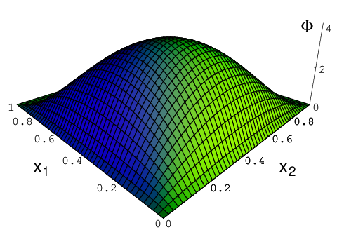
In Fig. 1 the model results for the proton distribution amplitude Φ\Phi are shown. The resulting shape is quite similar to that of the symmetric asymptotic DA in Eq. (18).
Refer to caption
Figure 1: The proton distribution amplitude.

In Table 1 we list the ϕ(l,m,n)\phi^{(l,m,n)} moments up to the order M=l+m+n≤3M=l+m+n\leq 3 in comparison with different model calculations. At this order there are 20 moments out of which only 10 are independent. Despite the fact that Φ\Phi is normalized, one has to keep in mind that it is a distribution amplitude, not a probability density. Thus its moments cannot strictly be interpreted as mean values [27]. However, the first moments of Φ\Phi provide an indication on how the longitudinal momentum of the proton is partitioned among the valence quarks. Since ϕ(1,0,0)≈0.6\phi^{(1,0,0)}\approx 0.6 in the model of Ref. [34], this is the reason why it is claimed that with QCD sum rules about 60% of the proton longitudinal momentum is carried by the up quark with helicity parallel to that of the proton. From Table 1 we see that a quite different result is obtained in the light-cone quark model, a roughly symmetric result similar to the one considered in Ref. [40]. In fact, while starting from quite different assumptions, the LCWF used here and the model wave function of Ref. [40] have some common features. Besides the longitudinal momentum dependence of Lz=0L_{z}=0 part of the present LCWF giving rise to an almost symmetric DA, our model resembles the Gaussian fall-off as function of the quark transverse momentum at large xx of the wave function of Ref. [40] and both models are able, for example, to reproduce the nucleon form factors. As a matter of fact, the transverse-momentum dependence of the present-model LCWF has been studied in Ref. [73], showing that the ratio of the squared mean transverse momentum and the mean square transverse momentum of transverse momentum dependent parton distributions agrees within 10%10\% accuracy with the results obtained assuming a factorized gaussian form for the nucleon wave function.

Using these results, we can study the behaviour of proton DA calculated in our model after evolution from the initial low-scale of the model to higher scales. The initial scale, corresponding to the results shown in Table 1, has been fixed evolving back unpolarized data, until the valence distributions matches the condition that the second moment, i.e. the momentum fraction carried by the valence quarks, is equal to one. Using LO evolution equations, we find Q02=0.079Q^{2}_{0}=0.079 GeV2, with ΛQCD=0.232\Lambda_{{\rm QCD}}=0.232 GeV [69]. Although there is no rigorous relation between the QCD quarks and the constituent quarks, and a more fundamental description of the transition from soft to hard regimes would be very helpful, this strategy reflects the present state of the art for quark model calculations [83, 84, 85], and has been validated with a fair comparison to experiments (see, for example, Ref. [73]). The results for the first moments ϕ(l,m,n)\phi^{(l,m,n)} with l+m+n≤2l+m+n\leq 2 after evolution to Q2=1Q^{2}=1 GeV2 are shown in Table 2. Comparison with the analogous results from lattice estimates [45] is quite nice. Evolution has only a very small effect: a further evolution to Q2=4Q^{2}=4 GeV2 would only hardly modify the last digit of our result. This is in agreement with the logarithmic scale dependence predicted by Eq. (21) and the fact that already at the input scale the behaviour of our DA approaches that of the asymptotic DA.

Table 2: The moments ϕ(l,m,n)\phi^{(l,m,n)} of the proton DA at different scales. The asymptotic values (AS) of Eq. (18) (second column) are compared with the lattice results (LAT) [31] at the scale Q2=1Q^{2}=1 GeV2 (third column) and with the corresponding results from the present model calculation (PPB), after evolution from the initial scale Q02=0.079Q^{2}_{0}=0.079 GeV2 to Q2=1Q^{2}=1 GeV2 (last column).
(ll, mm, nn) AS     LAT PPB
(0  0  0)(0\;\;0\;\;0)\,  1\,1\,  1\,1\,  1\,1\,
(1  0  0)(1\;\;0\;\;0)\, 13−∼ 0.333\,{\textstyle{1\over 3}}{\ \lower 2.0pt\hbox{$-$}\mkern-13.0mu\raise 2.0pt\hbox{$\sim$}\ }0.333\,  0.3999​(37)​(139)\,0.3999(37)(139)\,  0.340\,0.340\,
(0  1  0)(0\;\;1\;\;0)\, 13−∼ 0.333{\textstyle{1\over 3}}{\ \lower 2.0pt\hbox{$-$}\mkern-13.0mu\raise 2.0pt\hbox{$\sim$}\ }0.333  0.2986​(11)​(52)\,0.2986(11)(52)\,  0.335\,0.335\,
(0  0  1)(0\;\;0\;\;1)\, 13−∼ 0.333{\textstyle{1\over 3}}{\ \lower 2.0pt\hbox{$-$}\mkern-13.0mu\raise 2.0pt\hbox{$\sim$}\ }0.333  0.3015​(32)​(106)\,0.3015(32)(106)\,  0.326\,0.326\,
(2  0  0)(2\;\;0\;\;0)\, 17−∼ 0.143{\textstyle{1\over 7}}{\ \lower 2.0pt\hbox{$-$}\mkern-13.0mu\raise 2.0pt\hbox{$\sim$}\ }0.143  0.1816​(64)​(212)\,0.1816(64)(212)\,  0.147\,0.147\,
(0  2  0)(0\;\;2\;\;0)\, 17−∼ 0.143{\textstyle{1\over 7}}{\ \lower 2.0pt\hbox{$-$}\mkern-13.0mu\raise 2.0pt\hbox{$\sim$}\ }0.143  0.1281​(32)​(106)\,0.1281(32)(106)\,  0.144\,0.144\,
(0  0  2)(0\;\;0\;\;2)\, 17−∼ 0.143{\textstyle{1\over 7}}{\ \lower 2.0pt\hbox{$-$}\mkern-13.0mu\raise 2.0pt\hbox{$\sim$}\ }0.143  0.1311​(113)​(382)\,0.1311(113)(382)\,  0.137\,0.137\,
(1  1  0)(1\;\;1\;\;0)\, 221−∼ 0.095{\textstyle{2\over 21}}{\ \lower 2.0pt\hbox{$-$}\mkern-13.0mu\raise 2.0pt\hbox{$\sim$}\ }0.095  0.1092​(67)​(219)\,0.1092(67)(219)\,  0.098\,0.098\,
(1  0  1)(1\;\;0\;\;1)\, 221−∼ 0.095{\textstyle{2\over 21}}{\ \lower 2.0pt\hbox{$-$}\mkern-13.0mu\raise 2.0pt\hbox{$\sim$}\ }0.095  0.1091​(41)​(152)\,0.1091(41)(152)\,  0.095\,0.095\,
(0  1  1)(0\;\;1\;\;1)\, 221−∼ 0.095{\textstyle{2\over 21}}{\ \lower 2.0pt\hbox{$-$}\mkern-13.0mu\raise 2.0pt\hbox{$\sim$}\ }0.095  0.0613​(89)​(319)\,0.0613(89)(319)\,  0.093\,0.093\,

V Transition distribution amplitudes in a meson-cloud model

The general matrix element describing the transition from a nucleon to a meson state reads [53]

⟨π|ϵi​j​k​qαi′​(z1​n)​[z1;z0]i′​i​qj′​jβ​(z2​n)​[z2;z0]j′​j​qγk′​(z3​n)​[z3;z0]k′​k|N⟩,\langle\pi|\epsilon^{ijk}q^{i^{\prime}}_{\alpha}(z_{1}n)[z_{1};z_{0}]_{i^{\prime}i}q^{j^{\prime}}j_{\beta}(z_{2}n)[z_{2};z_{0}]_{j^{\prime}j}q^{k^{\prime}}_{\gamma}(z_{3}n)[z_{3};z_{0}]_{k^{\prime}k}|N\rangle, (45)

where the Wilson lines [zi;z0][z_{i};z_{0}] are defined as in Eq. (3). In the following they will be neglected by assuming to work in the light-cone gauge A+=0A^{+}=0. The spinorial and Lorentz decomposition of the matrix element (45) follows the same line as in the case of the baryon DAs. In particular, for the p→π0p\rightarrow\pi^{0} transition the leading-twist TDAs can be defined as

4​ℱ​(⟨π0​(pπ)|ϵi​j​k​uαi​(z1​n)​uβj​(z2​n)​dγk​(z3​n)|p⁡(pp,λ)⟩)\displaystyle 4\mathcal{F}\bigg(\langle\pi^{0}(p_{\pi})|\epsilon^{ijk}u^{i}_{\alpha}(z_{1}n)u^{j}_{\beta}(z_{2}n)d^{k}_{\gamma}(z_{3}n)|p(p_{p},\lambda)\rangle\bigg)
=ifNfπ[V1p​π0(p̸C)α​β(N+)γ+A1p​π0(p̸γ5C)α​β(γ5N+)γ\displaystyle{}=i\frac{f_{N}}{f_{\pi}}\Big[V_{1}^{p\pi^{0}}(\not{p}C)_{\alpha\beta}(N^{+})_{\gamma}+A_{1}^{p\pi^{0}}(\not{p}\gamma^{5}C)_{\alpha\beta}(\gamma^{5}N^{+})_{\gamma}
+T1p​π0​(σp​μ​C)α​β​(γμ​N+)γ+M−1​V2p​π0​(p̸​C)α​β​(Δ̸⟂​N+)γ\displaystyle{}\quad+T_{1}^{p\pi^{0}}(\sigma_{p\mu}C)_{\alpha\beta}(\gamma^{\mu}N^{+})_{\gamma}+M^{-1}V_{2}^{p\pi^{0}}(\not{p}C)_{\alpha\beta}(\not{\Delta}_{\perp}N^{+})_{\gamma}
+M−1​A2p​π0​(p̸​γ5​C)α​β​(γ5​Δ̸⟂​N+)γ+M−1​T2p​π0​(σp​Δ⟂​C)α​β​(N+)γ\displaystyle{}\quad+M^{-1}A_{2}^{p\pi^{0}}(\not{p}\gamma^{5}C)_{\alpha\beta}(\gamma^{5}\not{\Delta}_{\perp}N^{+})_{\gamma}+M^{-1}T_{2}^{p\pi^{0}}(\sigma_{p\Delta_{\perp}}C)_{\alpha\beta}(N^{+})_{\gamma}
+M−1T3p​π0(σp​μC)α​β(σμ​Δ⟂N+)γ+M−2T4p​π0(σp​Δ⟂C)α​β(Δ̸⟂N+)γ],\displaystyle{}\quad+M^{-1}T_{3}^{p\pi^{0}}(\sigma_{p\mu}C)_{\alpha\beta}(\sigma^{\mu\Delta_{\perp}}N^{+})_{\gamma}+M^{-2}T_{4}^{p\pi^{0}}(\sigma_{p\Delta_{\perp}}C)_{\alpha\beta}(\not{\Delta}_{\perp}N^{+})_{\gamma}\Big], (46)

where the symbol ℱ\mathcal{F} represents the Fourier transform (like Eq. (6)) and fπf_{\pi} is the pion decay constant (fπ=2​Fπ=131f_{\pi}=\sqrt{2}F_{\pi}=131 MeV). In a reference frame with the zz-axis along the direction of the proton momentum, the pion momentum pπp_{\pi} and the proton momentum ppp_{p} have the following Sudakov decomposition

pp=(1+ξ)​p+M21+ξ​n,\displaystyle p_{p}=(1+\xi)p+\frac{M^{2}}{1+\xi}n, (47)
pπ=(1−ξ)​p+mπ2+Δ⟂21−ξ​n+𝚫⟂,\displaystyle p_{\pi}=(1-\xi)p+\frac{m_{\pi}^{2}+\Delta^{2}_{\perp}}{1-\xi}n+\boldsymbol{\Delta}_{\perp}, (48)

where Δ\Delta is the four-momentum transfer,

Δ=pπ−pp=−2​ξ​p+[mπ2+Δ⟂21−ξ−M21+ξ]​n+𝚫⟂,\displaystyle\Delta=p_{\pi}-p_{p}=-2\xi p+\bigg[\frac{m_{\pi}^{2}+\Delta^{2}_{\perp}}{1-\xi}-\frac{M^{2}}{1+\xi}\bigg]n+\boldsymbol{\Delta_{\perp}}, (49)

and ξ\xi is the skewness variable describing the loss of plus momentum of the initial hadron in the proton-to-meson transition, i.e.

ξ=−Δ⋅n2​P⋅n=−Δ+2​P+,with​P=12​(pp+pπ).\xi=-\frac{\Delta\cdot n}{2P\cdot n}=-\frac{\Delta^{+}}{2P^{+}},\quad\mbox{with}\;\;P=\frac{1}{2}(p_{p}+p_{\pi}). (50)

The TDAs are dimensionless functions and depend on (xi,ξ,Δ2)(x_{i},\xi,\Delta^{2}), where the fraction of quark plus momentum xix_{i} have support in [−1+ξ,1+ξ][-1+\xi,1+\xi] and

Δ2=−2​ξ​[mπ2+Δ⟂21−ξ−M21+ξ]−Δ⟂2.\Delta^{2}=-2\xi\left[\frac{m_{\pi}^{2}+\Delta_{\perp}^{2}}{1-\xi}-\frac{M^{2}}{1+\xi}\right]-\Delta_{\perp}^{2}. (51)

Restricting ourselves to the case ξ>0\xi>0, momentum conservation requires ∑ixi=2​ξ\sum_{i}x_{i}=2\xi. The fields with positive momentum fractions, xi≥0x_{i}\geq 0, describe creation of quarks, whereas those with negative fractions, xi≤0x_{i}\leq 0, the absorption of antiquarks. This leads to define three distinct kinematical regions: the ERBL region for xi≥0x_{i}\geq 0, and two DGLAP regions when x1≥0,x_{1}\geq 0, x2≥0,x_{2}\geq 0, x3≤0,x_{3}\leq 0, or x1≥0,x_{1}\geq 0, x2≤0,x_{2}\leq 0, x3≤0.x_{3}\leq 0. The names derive from the evolution equations which controls the scale dependence of the TDAs in the different regions.

Denoting the matrix element in left-hand side of Eq. (46) by Tα​β,γλT_{\alpha\beta,\gamma}^{\lambda}, we can derive the eight TDAs in terms of the following linear combinations of matrix elements

V1p​π0\displaystyle V_{1}^{p\pi_{0}} =\displaystyle= −i​121/4​1+ξ​(P+)3/2​fπfN​(T12,1↑+T21,1↑),\displaystyle-i\frac{1}{2^{1/4}\sqrt{1+\xi}(P^{+})^{3/2}}\frac{f_{\pi}}{f_{N}}\Big(T_{12,1}^{\uparrow}+T_{21,1}^{\uparrow}\Big), (52)
A1p​π0\displaystyle A_{1}^{p\pi_{0}} =\displaystyle= i​121/4​1+ξ​(P+)3/2​fπfN​(T12,1↑−T21,1↑),\displaystyle i\frac{1}{2^{1/4}\sqrt{1+\xi}(P^{+})^{3/2}}\frac{f_{\pi}}{f_{N}}\Big(T_{12,1}^{\uparrow}-T_{21,1}^{\uparrow}\Big), (53)
T1p​π0\displaystyle T_{1}^{p\pi_{0}} =\displaystyle= i​121/4​1+ξ​(P+)3/2​fπfN​[T11,2↑+(Δ⟂−)2Δ⟂2​T22,2↑],\displaystyle i\frac{1}{2^{1/4}\sqrt{1+\xi}(P^{+})^{3/2}}\frac{f_{\pi}}{f_{N}}\bigg[T_{11,2}^{\uparrow}+\frac{(\Delta^{-}_{\perp})^{2}}{\Delta_{\perp}^{2}}T_{22,2}^{\uparrow}\bigg], (54)
V2p​π0\displaystyle V_{2}^{p\pi_{0}} =\displaystyle= −i​M​Δ⟂−Δ⟂2​121/4​1+ξ​(P+)3/2​fπfN​(T12,2↑+T21,2↑),\displaystyle-i\frac{M\Delta^{-}_{\perp}}{\Delta_{\perp}^{2}}\frac{1}{2^{1/4}\sqrt{1+\xi}(P^{+})^{3/2}}\frac{f_{\pi}}{f_{N}}\Big(T_{12,2}^{\uparrow}+T_{21,2}^{\uparrow}\Big), (55)
A2p​π0\displaystyle A_{2}^{p\pi_{0}} =\displaystyle= −i​M​Δ⟂−Δ⟂2​121/4​1+ξ​(P+)3/2​fπfN​(T12,2↑−T21,2↑),\displaystyle-i\frac{M\Delta^{-}_{\perp}}{\Delta_{\perp}^{2}}\frac{1}{2^{1/4}\sqrt{1+\xi}(P^{+})^{3/2}}\frac{f_{\pi}}{f_{N}}\Big(T_{12,2}^{\uparrow}-T_{21,2}^{\uparrow}\Big), (56)
T2p​π0\displaystyle T_{2}^{p\pi_{0}} =\displaystyle= −i​MΔ⟂2​121/4​1+ξ​(P+)3/2​fπfN​[Δ⟂+​T11,1↑−Δ⟂−​T22,1↑],\displaystyle-i\frac{M}{\Delta_{\perp}^{2}}\frac{1}{2^{1/4}\sqrt{1+\xi}(P^{+})^{3/2}}\frac{f_{\pi}}{f_{N}}\left[\Delta^{+}_{\perp}\,T_{11,1}^{\uparrow}-\Delta^{-}_{\perp}\,T_{22,1}^{\uparrow}\right], (57)
T3p​π0\displaystyle T_{3}^{p\pi_{0}} =\displaystyle= i​MΔ⟂2​121/4​1+ξ​(P+)3/2​fπfN​[Δ⟂+​T11,1↑+Δ⟂−​T22,1↑],\displaystyle i\frac{M}{\Delta_{\perp}^{2}}\frac{1}{2^{1/4}\sqrt{1+\xi}(P^{+})^{3/2}}\frac{f_{\pi}}{f_{N}}\left[\Delta^{+}_{\perp}\,T_{11,1}^{\uparrow}+\Delta^{-}_{\perp}\,T_{22,1}^{\uparrow}\right], (58)
T4p​π0\displaystyle T_{4}^{p\pi_{0}} =\displaystyle= i​2​M2​(Δ⟂−)2(Δ⟂2)2​121/4​1+ξ​(P+)3/2​fπfN​T22,2↑,\displaystyle i\frac{2M^{2}(\Delta^{-}_{\perp})^{2}}{(\Delta_{\perp}^{2})^{2}}\frac{1}{2^{1/4}\sqrt{1+\xi}(P^{+})^{3/2}}\frac{f_{\pi}}{f_{N}}T_{22,2}^{\uparrow}, (59)

where Δ⟂±=Δx±i​Δy\Delta^{\pm}_{\perp}=\Delta_{x}\pm i\Delta_{y}.

In the following we focus on the study of the TDAs in the ERBL region, corresponding to probe the ψ3​q+q​q¯\psi_{3q+q\bar{q}} Fock-component of the nucleon wave function. The five-parton component of the nucleon state can be modeled using the meson-cloud model developed in Refs. [74, 75]. The basic assumption of the model is that the physical nucleon is made of a bare nucleon dressed by the surrounding meson cloud so that the nucleon state is decomposed according to the meson-baryon Fock-state expansion as a superposition of a bare nucleon, formed by three valence quarks, and states containing virtual mesons with recoiling baryons. These baryon-meson subsystems are assumed to include configurations with the baryon being a nucleon or a Δ\Delta and the accompanying meson being a pion as well as a vector meson such as the ρ\rho or the ω\omega. Being interested to the p→π0p\rightarrow\pi^{0} TDAs, here we will consider the meson-baryon components with a pion and a nucleon or a Δ\Delta, given by the following representation in the light-cone dynamics

|N(Bπ);pp,λ⟩\displaystyle|N(B\pi);p_{p},\lambda\rangle =\displaystyle= ∫d​y​d2​𝐤⟂​∫0y∏i=13d​ξiξi​∫0(1−y)∏i=45d​ξiξi​∫1[2​(2​π)3]4​∏i=15d2​𝐤i⟂′\displaystyle\int\mathrm{d}y\mathrm{d}^{2}\mathbf{k}_{\perp}\int_{0}^{y}\prod_{i=1}^{3}\frac{\mathrm{d}\xi_{i}}{\sqrt{\xi_{i}}}\int_{0}^{(1-y)}\prod_{i=4}^{5}\frac{\mathrm{d}\xi_{i}}{\sqrt{\xi_{i}}}\int\frac{1}{[2(2\pi)^{3}]^{4}}\prod_{i=1}^{5}\mathrm{d}^{2}\mathbf{k}^{\prime}_{i\perp} (60)
×δ⁡(y−∑i=13ξi)​δ(2)​(𝐤⟂−∑i=13𝐤i⟂′)​δ​(1−∑i=15ξi)​δ(2)​(∑i=15𝐤i⟂′)\displaystyle\times\delta\bigg(y-\sum_{i=1}^{3}\xi_{i}\bigg)\delta^{(2)}\bigg(\mathbf{k}_{\perp}-\sum_{i={1}}^{3}\mathbf{k}^{\prime}_{i\perp}\bigg)\delta\bigg(1-\sum_{i={1}}^{5}\xi_{i}\bigg)\delta^{(2)}\bigg(\sum_{i={1}}^{5}\mathbf{k}^{\prime}_{i\perp}\bigg)
×∑λ′∑λi,τi,ciϕλ′​0λ⁡(N,B​π)​(y,k⟂)​y⁡(1−y)​Ψ~λ′B,[f]​(y,𝐤⟂,{ξi,𝐤i⟂′;λi,τi,ci}i=1,⋯,3)\displaystyle\times\sum_{\lambda^{\prime}}\sum_{\lambda_{i},\tau_{i},c_{i}}\phi_{\lambda^{\prime}0}^{\lambda(N,B\pi)}(y,\textbf{k}_{\perp})\sqrt{y(1-y)}\tilde{\Psi}_{\lambda^{\prime}}^{B,[f]}(y,\mathbf{k}_{\perp};\{\xi_{i},\mathbf{k}^{\prime}_{i\perp};\lambda_{i},\tau_{i},c_{i}\}_{i=1,\cdots,3})
×Ψ~π,[f](1−y,−𝐤⟂;{ξi,𝐤i⟂′;λi,τi}i=4,5)∏i=15|ξipp+,𝐤i⟂′+ξi𝐩p⟂,λi,τi,ci;q⟩,\displaystyle\times\tilde{\Psi}^{\pi,[f]}(1-y,-\mathbf{k}_{\perp};\{\xi_{i},\mathbf{k}^{\prime}_{i\perp};\lambda_{i},\tau_{i}\}_{i=4,5})\prod_{i={1}}^{5}|\xi_{i}p_{p}^{+},\mathbf{k}^{\prime}_{i\perp}+\xi_{i}\mathbf{p}_{p\perp},\lambda_{i},\tau_{i},c_{i};q\rangle,

where the LCWF of the baryon, Ψ~λ′B,[f]\tilde{\Psi}^{B,[f]}_{\lambda^{\prime}}, and the pion, Ψ~π,[f]\tilde{\Psi}^{\pi,[f]}, incorporate the Jacobian 𝒥{\cal J} of the transformation from the intrinsic variables with respect to the hadron rest-frame ({ζi,𝜿i⟂}\{\zeta_{i},\boldsymbol{\kappa}_{i\perp}\}) to the intrinsic variables with respect to the nucleon rest frame ({ξi,𝐤i⟂′}\{\xi_{i},\mathbf{k}^{\prime}_{i\perp}\}), i.e.

Ψ~λ′B,[f]​({ξi,𝐤i⟂′;λi,τi}i=1,2,3)\displaystyle\tilde{\Psi}_{\lambda^{\prime}}^{B,\,[f]}(\{\xi_{i},{\bf k}^{\prime}_{i\perp};\lambda_{i},\tau_{i}\}_{i=1,2,3}) =\displaystyle= 𝒥⁡(ξ1,ξ2,ξ3)​Ψ~λ′B,[f]​({ζi,𝜿i⟂;λi,τi}i=1,2,3)\displaystyle\sqrt{{\cal J}(\xi_{1},\xi_{2},\xi_{3})}\tilde{\Psi}_{\lambda^{\prime}}^{B,\,[f]}(\{\zeta_{i},\boldsymbol{\kappa}_{i\perp};\lambda_{i},\tau_{i}\}_{i=1,2,3}) (61)
=\displaystyle= 1y3/2​Ψ~λ′B,[f]​({ζi,𝜿i⟂;λi,τi}i=1,2,3),\displaystyle\frac{1}{y^{3/2}}\tilde{\Psi}_{\lambda^{\prime}}^{B,\,[f]}(\{\zeta_{i},\boldsymbol{\kappa}_{i\perp};\lambda_{i},\tau_{i}\}_{i=1,2,3}),
Ψ~π,[f]​({ξi,𝐤i⟂′;λi,τi}i=4,5)\displaystyle\tilde{\Psi}^{\pi,\,[f]}(\{\xi_{i},{\bf k}^{\prime}_{i\perp};\lambda_{i},\tau_{i}\}_{i=4,5}) =\displaystyle= 𝒥⁡(ξ4,ξ5)​Ψ~π,[f]​({ζi,𝜿i⟂;λi,τi}i=4,5)\displaystyle\sqrt{{\cal J}(\xi_{4},\xi_{5})}\tilde{\Psi}^{\pi,\,[f]}(\{\zeta_{i},\boldsymbol{\kappa}_{i\perp};\lambda_{i},\tau_{i}\}_{i=4,5}) (62)
=\displaystyle= 1(1−y)​Ψ~π,[f]​({ζi,𝜿i⟂;λi,τi}i=4,5).\displaystyle\frac{1}{(1-y)}\tilde{\Psi}^{\pi,\,[f]}(\{\zeta_{i},\boldsymbol{\kappa}_{i\perp};\lambda_{i},\tau_{i}\}_{i=4,5}).

The relations between the variables ({xi,𝐤i⟂}\{x_{i},\mathbf{k}_{i\perp}\}) and {ξi,𝐤i⟂′}\{\xi_{i},\mathbf{k}^{\prime}_{i\perp}\}, are given by:

For i=1,2,3i=1,2,3, corresponding to the indices of the three quarks in the baryon,

ζi=ξiy,𝜿i⟂=𝐤i⟂′−ζi​𝐤⟂;\displaystyle\zeta_{i}=\frac{\xi_{i}}{y},\qquad\boldsymbol{\kappa}_{i\perp}={\bf k}^{\prime}_{i\perp}-\zeta_{i}\,{\bf k}_{\perp}; (63)

For i=4,5i=4,5, corresponding to the indices of the quark and antiquark in the pion, respectively:

ζi=ξi(1−y),𝜿i⟂=𝐤i⟂′+ζi​𝐤⟂.\displaystyle\zeta_{i}=\frac{\xi_{i}}{(1-y)},\qquad\boldsymbol{\kappa}_{i\perp}={\bf k}^{\prime}_{i\perp}+\zeta_{i}\,{\bf k}_{\perp}. (64)

In Eq. (60) the function ϕλ′​0λ⁡(N,B​π)​(y,𝐤⟂)\phi_{\lambda^{\prime}0}^{\lambda\,(N,B\pi)}(y,{\mathbf{k}}_{\perp}) is the probability amplitude to find a physical nucleon with helicity λ\lambda in a state consisting of a virtual baryon B=N,ΔB=N,\Delta and a virtual pion, with the baryon having helicity λ′\lambda^{\prime}, longitudinal momentum fraction yy and transverse momentum 𝐤⟂{\mathbf{k}}_{\perp}, and the pion having longitudinal momentum fraction 1−y1-y and transverse momentum −𝐤⟂-{\mathbf{k}}_{\perp}. This splitting function can be calculated using time-ordered perturbation theory in the infinite momentum frame as explained in Ref. [86], and have also been rederived and tabulated in Ref. [74].

For the pion state in the matrix element of Eq. (46) we consider the valence q​q¯q\bar{q} component given by

|π⁡(pπ)⟩=∑τi,λi,ci∫[d​ξξ]2​[d2​𝐤⟂]2​Ψπ,[f]​({ξi,𝐤i⟂;λi,τi}i=1,2)​∏i=12|qλi;ξip+π,𝐩i⟂⟩,\hbox{$|\pi(p_{\pi})\rangle$}=\sum_{\tau_{i},\lambda_{i},c_{i}}\int\left[\frac{{\rm d}\xi}{\sqrt{\xi}}\right]_{2}[{\rm d}^{2}{\bf k}_{\perp}]_{2}\Psi^{\pi,[f]}(\{\xi_{i},{\bf k}_{i\perp};\lambda_{i},\tau_{i}\}_{i=1,2})\prod_{i=1}^{2}\hbox{$|q^{\lambda_{i}};\xi_{i}p^{+}_{\pi},\,{\bf p}_{i\perp}\rangle$}, (65)

where 𝐩⟂i=𝐤i⟂+ξi​pπ+{\bf p}_{\perp i}={\bf k}_{i\perp}+\xi_{i}p^{+}_{\pi} and the q​q¯q\bar{q} state is defined as

∏i=12|qλi;k~i⟩=δi​j3​bq†i​(k~1,λ1)​dq†j​(k~2,λ2)​|0⟩.\prod_{i=1}^{2}\hbox{$|q^{\lambda_{i}};\tilde{k}_{i}\rangle$}=\frac{\delta_{ij}}{\sqrt{3}}b_{q}^{\dagger i}(\tilde{k}_{1},\lambda_{1})d_{q}^{\dagger j}(\tilde{k}_{2},\lambda_{2})|0\rangle. (66)

Using the expressions for the proton and pion state given in Eqs. (60) and (65), and the momentum-space expansion (26) of the quark fields, combined with the anticommutation relations for the quark creation and annihilation operators, the final expression for the matrix elements Tα,β​γλT^{\lambda}_{\alpha,\beta\gamma} is given by

Tα,β​γλ=\displaystyle T^{\lambda}_{\alpha,\beta\gamma}= −24​(12​ξ)3/2​1x1​x2​x3​u+α​(k1+,λ1)​u+β​(k2+,λ2)​u+γ​(k3+,λ3)\displaystyle{}-24\left(\frac{1}{2\xi}\right)^{3/2}\frac{1}{\sqrt{x_{1}x_{2}x_{3}}}u_{+\alpha}(k^{+}_{1},\lambda_{1})u_{+\beta}(k^{+}_{2},\lambda_{2})u_{+\gamma}(k^{+}_{3},\lambda_{3})
×∑B∑λ′∫d​y​d2​𝐤⟂​ϕλ′​0λ⁡(N,B​π)​(y,k⟂)​y⁡(1−y)​δ​(1−y−pπ+pp+)​δ(2)​(𝐤⟂+𝐩π⟂)\displaystyle{}\times\sum_{B}\sum_{\lambda^{\prime}}\int\mathrm{d}y\mathrm{d}^{2}\mathbf{k}_{\perp}\phi_{\lambda^{\prime}0}^{\lambda(N,B\pi)}(y,\textbf{k}_{\perp})\sqrt{y(1-y)}\delta\bigg(1-y-\frac{p_{\pi}^{+}}{p_{p}^{+}}\bigg)\delta^{(2)}\bigg(\mathbf{k}_{\perp}+\mathbf{p}_{\pi\perp}\bigg)
×∫[d2𝜿⟂]3Ψ~λ′B,[f]({x12​ξ,𝜿1⟂;λ1,1/2}{x22​ξ,𝜿2⟂;λ2,1/2}{x32​ξ,𝜿3⟂;λ3,−1/2}).\displaystyle{}\times\int[\mathrm{d}^{2}\boldsymbol{\kappa}_{\perp}]_{3}\,\tilde{\Psi}_{\lambda^{\prime}}^{B,[f]}\bigg(\{\frac{x_{1}}{2\xi},\boldsymbol{\kappa}_{1\perp};\lambda_{1},1/2\}\{\frac{x_{2}}{2\xi},\boldsymbol{\kappa}_{2\perp};\lambda_{2},1/2\}\{\frac{x_{3}}{2\xi},\boldsymbol{\kappa}_{3\perp};\lambda_{3},-1/2\}\bigg).

The light-cone spinors of the quarks are defined as in Eq. (33), and depend on the longitudinal momenta ki+=xi​P+k^{+}_{i}=x_{i}P^{+}. The Dirac indices α,\alpha, β,\beta, and γ\gamma fix the total quark helicity of the baryon wave function, as explained in sect. II, while the isospin quantum numbers in the baryon wave function correspond to the u​u​duud configuration. Eq. () has a clear physical interpretation and allows to relate the nucleon-to-pion TDAs to the baryon distribution amplitudes in the (B​π)(B\pi) component of the nucleon weighted by the probability amplitude that the nucleon fluctuates in the corresponding (B​π)(B\pi) subsytem with the pion momentum matching the pion momentum in the final state. The momentum fraction of the quarks in the baryon LCWF are defined with respect to the longitudinal momentum of the baryon, i.e. κi+/(y​pp+)=xi/(2​ξ)\kappa^{+}_{i}/(yp^{+}_{p})=x_{i}/(2\xi), while the integration over the transverse quark momenta corresponds to the projection of the baryon LCWF onto the zero orbital angular momentum component. In Eq. (), the sum over the baryon states is restricted to the nucleon and the Δ\Delta, while the sum over the helicity λ′\lambda^{\prime} of the baryon permits baryon-pion fluctuations which do not conserve the helicity of the parent nucleon.

In the case of the nucleon contribution, we model the proton LCWF as in Eq. (38), with parameters γ=3.21\gamma=3.21, β=0.489\beta=0.489 GeV and m=0.264m=0.264 GeV from the fit of the valence and meson-cloud contribution to the electroweak nucleon form factors [75]. The Δ\Delta is described as a state of isospin τ=32\tau={\textstyle{3\over 2}} obtained as a pure splin-flip excitation of the nucleon, with the same momentum-dependent wave function of the nucleon, i.e.

ΨλΔ,[f]​({xi},{ki},{λi},{u​u​d})\displaystyle\Psi^{\Delta,[f]}_{\lambda}(\{x_{i}\},\{k_{i}\},\{\lambda_{i}\},\{uud\}) =\displaystyle= ψ~​({xi,𝐤i⟂})​ΞλΔ​(λ1,λ2,λ3)​Φ~32​121​(12,12,−12),\displaystyle\tilde{\psi}(\{x_{i},{\bf k}_{i\perp}\})\Xi_{\lambda}^{\Delta}(\lambda_{1},\lambda_{2},\lambda_{3})\tilde{\Phi}^{1}_{{\textstyle{3\over 2}}{\textstyle{1\over 2}}}({\textstyle{1\over 2}},{\textstyle{1\over 2}},-{\textstyle{1\over 2}}), (68)

with the isospin coefficient Φ~32​121​(12,12,−12)=13\tilde{\Phi}^{1}_{{\textstyle{3\over 2}}{\textstyle{1\over 2}}}(\frac{1}{2},\frac{1}{2},-\frac{1}{2})=\sqrt{\frac{1}{3}} and the spin dependent part given by

ΞλΔ(λ1,λ2,λ3)=∑μ1​μ2​μ3Dμ1​λ11/2∗(Rc​f(k~1))Dμ2​λ21/2∗(Rc​f(k~2))Dμ3​λ31/2∗(Rc​f(k~3))Φ~32​λ1(μ1,μ2,μ3).\displaystyle\Xi_{\lambda}^{\Delta}(\lambda_{1},\lambda_{2},\lambda_{3})=\sum_{\mu_{1}\mu_{2}\mu_{3}}D_{\mu_{1}\lambda_{1}}^{1/2*}(R_{cf}(\tilde{k}_{1}))D_{\mu_{2}\lambda_{2}}^{1/2*}(R_{cf}(\tilde{k}_{2}))D_{\mu_{3}\lambda_{3}}^{1/2*}(R_{cf}(\tilde{k}_{3}))\tilde{\Phi}^{1}_{{\textstyle{3\over 2}}\lambda}(\mu_{1},\mu_{2},\mu_{3}). (69)

The explicit expression of the functions ΞλΔ\Xi_{\lambda}^{\Delta} for all the possible spin configurations of the three quarks in the Δ\Delta state is given in the Appendix.
Finally, the splitting function ϕλ​0(N,B​π)\phi^{(N,B\pi)}_{\lambda 0} in Eq. () is calculated as in Ref. [75].

Inserting the matrix elements Tα,β​γλT^{\lambda}_{\alpha,\beta\gamma} from Eq. () into Eqs. (52)-(59) we finally obtain the expressions of the TDAs in the meson-cloud model:

V1p​π0\displaystyle V_{1}^{p\pi_{0}} =\displaystyle= i​4​32​ξ​(1−ξ)(1+ξ)3​fπfN​∫[d2​𝐤⟂]3​ψ~​({xi,𝐤i⟂})\displaystyle i\frac{4\sqrt{3}}{2\xi}\sqrt{\frac{(1-\xi)}{(1+\xi)^{3}}}\frac{f_{\pi}}{f_{N}}\int[\mathrm{d}^{2}\mathbf{k}_{\perp}]_{3}\tilde{\psi}(\{x_{i},\mathbf{k}_{i\perp}\}) (70)
×{ϕ↑0↑(N,N​π)(y,−pπ⟂)[Ξ↑N(↑,↓,↑)+Ξ↑N(↓,↑,↑)]+ϕ↑0↑(N,Δ​π)(y,−pπ⟂)[Ξ↑Δ(↑,↓,↑)+Ξ↑Δ(↓,↑,↑)]},\displaystyle\times\left\{\phi_{\uparrow 0}^{\uparrow(N,N\pi)}(y,-\textbf{p}_{\pi\perp})\left[\Xi^{N}_{\uparrow}(\uparrow,\downarrow,\uparrow)+\Xi^{N}_{\uparrow}(\downarrow,\uparrow,\uparrow)\right]+\phi_{\uparrow 0}^{\uparrow(N,\Delta\pi)}(y,-\textbf{p}_{\pi\perp})\left[\Xi^{\Delta}_{\uparrow}(\uparrow,\downarrow,\uparrow)+\Xi^{\Delta}_{\uparrow}(\downarrow,\uparrow,\uparrow)\right]\right\},
A1p​π0\displaystyle A_{1}^{p\pi_{0}} =\displaystyle= −i4​32​ξ(1−ξ)(1+ξ)3fπfN∫[d2𝐤⟂]3ψ~({xi,𝐤i⟂})\displaystyle-i\frac{4\sqrt{3}}{2\xi}\sqrt{\frac{(1-\xi)}{(1+\xi)^{3}}}\frac{f_{\pi}}{f_{N}}\int[\mathrm{d}^{2}\mathbf{k}_{\perp}]_{3}\tilde{\psi}(\{x_{i},\mathbf{k}_{i\perp}\}) (71)
×{ϕ↑0↑(N,N​π)(y,−pπ⟂)[Ξ↑N(↑,↓,↑)−Ξ↑N(↓,↑,↑)]+ϕ↑0↑(N,Δ​π)(y,−pπ⟂)[Ξ↑Δ(↑,↓,↑)−Ξ↑Δ(↓,↑,↑)]},\displaystyle\times\left\{\phi_{\uparrow 0}^{\uparrow(N,N\pi)}(y,-\textbf{p}_{\pi\perp})\left[\Xi^{N}_{\uparrow}(\uparrow,\downarrow,\uparrow)-\Xi^{N}_{\uparrow}(\downarrow,\uparrow,\uparrow)\right]+\phi_{\uparrow 0}^{\uparrow(N,\Delta\pi)}(y,-\textbf{p}_{\pi\perp})\left[\Xi^{\Delta}_{\uparrow}(\uparrow,\downarrow,\uparrow)-\Xi^{\Delta}_{\uparrow}(\downarrow,\uparrow,\uparrow)\right]\right\},
T1p​π0\displaystyle T_{1}^{p\pi_{0}} =\displaystyle= −i4​32​ξ(1−ξ)(1+ξ)3fπfN∫[d2𝐤⟂]3ψ~({xi,𝐤i⟂}){ϕ↑0↑(N,N​π)(y,−pπ⟂)Ξ↑N(↑,↑,↓)\displaystyle-i\frac{4\sqrt{3}}{2\xi}\sqrt{\frac{(1-\xi)}{(1+\xi)^{3}}}\frac{f_{\pi}}{f_{N}}\int[\mathrm{d}^{2}\mathbf{k}_{\perp}]_{3}\tilde{\psi}(\{x_{i},\mathbf{k}_{i\perp}\})\left\{\phi_{\uparrow 0}^{\uparrow(N,N\pi)}(y,-\textbf{p}_{\pi\perp})\Xi^{N}_{\uparrow}(\uparrow,\uparrow,\downarrow)\right. (72)
+ϕ↑0↑(N,Δ​π)(y,−pπ⟂)Ξ↑Δ(↑,↑,↓)+(Δ⟂−)2Δ⟂2ϕ⇓0↑(N,Δ​π)(y,−pπ⟂)Ξ⇓Δ(↓,↓,↓)},\displaystyle\left.+\phi_{\uparrow 0}^{\uparrow(N,\Delta\pi)}(y,-\textbf{p}_{\pi\perp})\Xi^{\Delta}_{\uparrow}(\uparrow,\uparrow,\downarrow)+\frac{(\Delta^{-}_{\perp})^{2}}{\Delta_{\perp}^{2}}\phi_{\Downarrow 0}^{\uparrow(N,\Delta\pi)}(y,-\textbf{p}_{\pi\perp})\Xi^{\Delta}_{\Downarrow}(\downarrow,\downarrow,\downarrow)\right\},
V2p​π0\displaystyle V_{2}^{p\pi_{0}} =\displaystyle= i​4​32​ξ​(1−ξ)(1+ξ)3​fπfN​M​Δ⟂−Δ⟂2​∫[d2​𝐤⟂]3​ψ~​({xi,𝐤i⟂})\displaystyle i\frac{4\sqrt{3}}{2\xi}\sqrt{\frac{(1-\xi)}{(1+\xi)^{3}}}\frac{f_{\pi}}{f_{N}}\frac{M\Delta^{-}_{\perp}}{\Delta_{\perp}^{2}}\int[\mathrm{d}^{2}\mathbf{k}_{\perp}]_{3}\tilde{\psi}(\{x_{i},\mathbf{k}_{i\perp}\}) (73)
×{ϕ↓0↑(N,N​π)(y,−pπ⟂)[Ξ↓N(↑,↓,↓)+Ξ↓N(↓,↑,↓)]+ϕ↓0↑(N,Δ​π)(y,−pπ⟂)[Ξ↓Δ(↑,↓,↓)+Ξ↓Δ(↓,↑,↓)]},\displaystyle\times\left\{\phi_{\downarrow 0}^{\uparrow(N,N\pi)}(y,-\textbf{p}_{\pi\perp})\left[\Xi^{N}_{\downarrow}(\uparrow,\downarrow,\downarrow)+\Xi^{N}_{\downarrow}(\downarrow,\uparrow,\downarrow)\right]+\phi_{\downarrow 0}^{\uparrow(N,\Delta\pi)}(y,-\textbf{p}_{\pi\perp})\left[\Xi^{\Delta}_{\downarrow}(\uparrow,\downarrow,\downarrow)+\Xi^{\Delta}_{\downarrow}(\downarrow,\uparrow,\downarrow)\right]\right\},
A2p​π0\displaystyle A_{2}^{p\pi_{0}} =\displaystyle= i​4​32​ξ​(1−ξ)(1+ξ)3​fπfN​M​Δ⟂−Δ⟂2​∫[d2​𝐤⟂]3​ψ~​({xi,𝐤i⟂})\displaystyle i\frac{4\sqrt{3}}{2\xi}\sqrt{\frac{(1-\xi)}{(1+\xi)^{3}}}\frac{f_{\pi}}{f_{N}}\frac{M\Delta^{-}_{\perp}}{\Delta_{\perp}^{2}}\int[\mathrm{d}^{2}\mathbf{k}_{\perp}]_{3}\tilde{\psi}(\{x_{i},\mathbf{k}_{i\perp}\}) (74)
×{ϕ↓0↑(N,N​π)(y,−pπ⟂)[Ξ↓N(↑,↓,↓)−Ξ↓N(↓,↑,↓)]+ϕ↓0↑(N,Δ​π)(y,−pπ⟂)[Ξ↓Δ(↑,↓,↓)−Ξ↓Δ(↓,↑,↓)]},\displaystyle\times\left\{\phi_{\downarrow 0}^{\uparrow(N,N\pi)}(y,-\textbf{p}_{\pi\perp})\left[\Xi^{N}_{\downarrow}(\uparrow,\downarrow,\downarrow)-\Xi^{N}_{\downarrow}(\downarrow,\uparrow,\downarrow)\right]+\phi_{\downarrow 0}^{\uparrow(N,\Delta\pi)}(y,-\textbf{p}_{\pi\perp})\left[\Xi^{\Delta}_{\downarrow}(\uparrow,\downarrow,\downarrow)-\Xi^{\Delta}_{\downarrow}(\downarrow,\uparrow,\downarrow)\right]\right\},
T2p​π0\displaystyle T_{2}^{p\pi_{0}} =\displaystyle= i4​32​ξ(1−ξ)(1+ξ)3fπfN∫[d2𝐤⟂]3ψ~({xi,𝐤i⟂}){−Δ⟂−ϕ↓0↑(N,N​π)(y,−pπ⟂)Ξ↓N(↓,↓,↑)\displaystyle i\frac{4\sqrt{3}}{2\xi}\sqrt{\frac{(1-\xi)}{(1+\xi)^{3}}}\frac{f_{\pi}}{f_{N}}\int[\mathrm{d}^{2}\mathbf{k}_{\perp}]_{3}\tilde{\psi}(\{x_{i},\mathbf{k}_{i\perp}\})\left\{-\Delta^{-}_{\perp}\,\phi_{\downarrow 0}^{\uparrow(N,N\pi)}(y,-\textbf{p}_{\pi\perp})\Xi^{N}_{\downarrow}(\downarrow,\downarrow,\uparrow)\right. (75)
+Δ⟂+ϕ⇑0↑(N,Δ​π)(y,−pπ⟂)Ξ⇑Δ(↑,↑,↑)−Δ⟂−ϕ↓0↑(N,Δ​π)(y,−pπ⟂)Ξ↓Δ(↓,↓,↑)},\displaystyle\left.+\Delta^{+}_{\perp}\ \phi_{\Uparrow 0}^{\uparrow(N,\Delta\pi)}(y,-\textbf{p}_{\pi\perp})\Xi^{\Delta}_{\Uparrow}(\uparrow,\uparrow,\uparrow)-\Delta^{-}_{\perp}\,\phi_{\downarrow 0}^{\uparrow(N,\Delta\pi)}(y,-\textbf{p}_{\pi\perp})\Xi^{\Delta}_{\downarrow}(\downarrow,\downarrow,\uparrow)\right\},
T3p​π0\displaystyle T_{3}^{p\pi_{0}} =\displaystyle= −i4​32​ξ(1−ξ)(1+ξ)3fπfN∫[d2𝐤⟂]3ψ~({xi,𝐤i⟂}){Δ⟂−ϕ↓0↑(N,N​π)(y,−pπ⟂)Ξ↓N(↓,↓,↑)\displaystyle-i\frac{4\sqrt{3}}{2\xi}\sqrt{\frac{(1-\xi)}{(1+\xi)^{3}}}\frac{f_{\pi}}{f_{N}}\int[\mathrm{d}^{2}\mathbf{k}_{\perp}]_{3}\tilde{\psi}(\{x_{i},\mathbf{k}_{i\perp}\})\left\{\Delta^{-}_{\perp}\,\phi_{\downarrow 0}^{\uparrow(N,N\pi)}(y,-\textbf{p}_{\pi\perp})\Xi^{N}_{\downarrow}(\downarrow,\downarrow,\uparrow)\right. (76)
+Δ⟂+ϕ⇑0↑(N,Δ​π)(y,−pπ⟂)Ξ⇑Δ(↑,↑,↑)+Δ⟂−ϕ↓0↑(N,Δ​π)(y,−pπ⟂)Ξ↓Δ(↓,↓,↑)},\displaystyle\left.+\Delta^{+}_{\perp}\ \phi_{\Uparrow 0}^{\uparrow(N,\Delta\pi)}(y,-\textbf{p}_{\pi\perp})\Xi^{\Delta}_{\Uparrow}(\uparrow,\uparrow,\uparrow)+\Delta^{-}_{\perp}\,\phi_{\downarrow 0}^{\uparrow(N,\Delta\pi)}(y,-\textbf{p}_{\pi\perp})\Xi^{\Delta}_{\downarrow}(\downarrow,\downarrow,\uparrow)\right\},
T4p​π0\displaystyle T_{4}^{p\pi_{0}} =\displaystyle= −i4​32​ξ(1−ξ)(1+ξ)3fπfN2​M2​(Δ⟂−)2(Δ⟂2)2∫[d2𝐤⟂]3ψ~({xi,𝐤i⟂})ϕ⇓0↑(N,Δ​π)(y,−pπ⟂)Ξ⇓Δ(↓,↓,↓),\displaystyle-i\frac{4\sqrt{3}}{2\xi}\sqrt{\frac{(1-\xi)}{(1+\xi)^{3}}}\frac{f_{\pi}}{f_{N}}\frac{2M^{2}(\Delta^{-}_{\perp})^{2}}{(\Delta_{\perp}^{2})^{2}}\int[\mathrm{d}^{2}\mathbf{k}_{\perp}]_{3}\tilde{\psi}(\{x_{i},\mathbf{k}_{i\perp}\})\phi_{\Downarrow 0}^{\uparrow(N,\Delta\pi)}(y,-\textbf{p}_{\pi\perp})\Xi^{\Delta}_{\Downarrow}(\downarrow,\downarrow,\downarrow), (77)

where the longitudinal momentum fraction in the argument of the splitting function is y=2​ξ/(1+ξ)y=2\xi/(1+\xi) and the spin 32{\textstyle{3\over 2}} (−32-{\textstyle{3\over 2}}) state of the Δ\Delta is indicated as ⇑\Uparrow (⇓\Downarrow).

VI Some results for the TDAs

As an example results are reported in Figs. 2 and 3 under kinematic conditions relevant in the case of hard exclusive electroproduction of a pion in the backward region [56] or in associated production of a pion and a high-Q2Q^{2} dilepton pair in p​p¯p\bar{p} annihilation [63]. Preliminary results for other kinematics have been presented in Ref. [88].

The vector and axial-vector TDAs in Fig. 2 exhibit the expected symmetric and antisymmetric behaviour under permutation of the two up quarks, respectively. The Δ\Delta contribution has the same shape as the proton contribution, with the same sign for A1p​πA^{p\pi}_{1} and V2p​πV^{p\pi}_{2}, and opposite sign for V1p​πV^{p\pi}_{1} and A2p​πA^{p\pi}_{2}. The relative contribution of the nucleon with respect to the Δ\Delta is always smaller in absolute value for the vector TDAs, being suppressed by a factor of about 10 in the case of V1p​πV^{p\pi}_{1} and by a factor of about 1.5 in the case of V2p​πV^{p\pi}_{2}. Viceversa, for the axial-vector TDAs one finds that the nucleon contribution to A1p​πA^{p\pi}_{1} is smaller than the Δ\Delta contribution by a factor 3, while for A2p​πA^{p\pi}_{2} the weight of the nucleon contribution is three times larger than in the case of the Δ.\Delta. This can be traced back both to the different spin structure and to the different splitting functions in Eqs. (70)-(71), and (73)-(74). In particular, V1p​πV^{p\pi}_{1} and A1p​πA^{p\pi}_{1} involve splitting functions without flip of the helicity of the parent nucleon, while V2p​πV^{p\pi}_{2} and A2p​πA^{p\pi}_{2} are proportional to splitting functions with helicity flip. In the explored kinematics, the (N,N​π)(N,N\pi) vertex without helicity flip is suppressed by a factor 5 with respect to the (N,Δ​π)(N,\Delta\pi) interaction, while for the opposite case with helicity flip the probability amplitude to have a (N​π)(N\pi) fluctuation in the nucleon is almost twice larger than for the (Δ​π)(\Delta\pi) subsystem.

The tensor TDAs in Fig. 3 are symmetric under permutation of the two up quarks and, at variance with the other TDAs, involve spin configurations also with parallel helicities of all three quarks. Such spin configurations receive contribution only from the Δ\Delta with helicity Jz=±3/2J_{z}=\pm 3/2 because of the projection of the baryon wave function in Eqs. (72) and (75)-(77) onto the zero orbital angular momentum component. In particular, one finds that in the explored kinematics the splitting function of the nucleon into a Δ\Delta with helicity Jz=3/2J_{z}=3/2 is 10 times bigger than in the case with helicity Jz=−3/2J_{z}=-3/2, and with opposite sign. Furthermore, these terms are multiplied by kinematical coefficients which modulate their relative contribution to the tensor TDAs in a quite different way. For example, the contribution of the Δ\Delta state with helicity Jz=3/2J_{z}=3/2 is quite small in the case of T1p​πT^{p\pi}_{1}, while it is enhanced by an additional factor of 2​M2/Δ⟂2−∼ 502M^{2}/\Delta^{2}_{\perp}{\ \lower 2.0pt\hbox{$-$}\mkern-13.0mu\raise 2.0pt\hbox{$\sim$}\ }50 in T4p​π.T^{p\pi}_{4}. This is the only non-vanishing contribution to T4p​πT^{p\pi}_{4}. In T1p​πT^{p\pi}_{1} there is also the contribution from the helicity states Jz=1/2,J_{z}=1/2, with the same sign for the nucleon and the Δ\Delta, but larger by about a factor 10 in the case of Δ\Delta. In the case of T2p​πT^{p\pi}_{2} and T3p​πT^{p\pi}_{3} the contribution from the Δ\Delta is large, and it is mainly given by the configuration with helicity Jz=3/2J_{z}=3/2. However, this contribution is reduced by that of the proton with a similar shape in the case of T2p​πT^{p\pi}_{2}, whereas 2/3 of T3p​πT^{p\pi}_{3} are due to the proton and 1/3 to the Δ\Delta.

Refer to captionRefer to captionRefer to captionRefer to caption
Figure 2: The p→π0p\rightarrow\pi^{0} transition distribution amplitudes V1p​πV^{p\pi}_{1} (up left), A1p​πA^{p\pi}_{1} (up right), V2p​πV^{p\pi}_{2} (down left), A2p​πA^{p\pi}_{2} (down right) as function of (x1,x2,2​ξ−x1−x2)(x_{1},x_{2},2\xi-x_{1}-x_{2}) at fixed ξ=0.9\xi=0.9 and Δ2=−0.1\Delta^{2}=-0.1 GeV2.
Refer to captionRefer to captionRefer to captionRefer to caption
Figure 3: The p→π0p\rightarrow\pi^{0} transition distribution amplitudes T1p​πT^{p\pi}_{1} (up left), T2p​πT^{p\pi}_{2} (up right), T3p​πT^{p\pi}_{3} (down left), and T4p​πT^{p\pi}_{4} (down left) as function of (x1,x2,2​ξ−x1−x2)(x_{1},x_{2},2\xi-x_{1}-x_{2}) at fixed ξ=0.9\xi=0.9 and Δ2=−0.1\Delta^{2}=-0.1 GeV2.

VII Concluding remarks

In the light-cone description the nucleon state is decomposed in terms of NN-parton Fock states with coefficients representing the momentum light-cone wave function of the NN partons. Since the constituent quark models work so well phenomenologically, in applications it is usually assumed that only the Fock components with a few partons have to be taken into account. One of such models has been studied in a series of papers to show that the parametrization of the LCWF up to five-parton components is already sufficient to account for the electroweak form factors [75] and spin densities [70] of the nucleon, as well as the observed asymmetries due to transverse momentum dependence of parton distributions [72, 73], and to give a useful insight into the quark generalized parton distributions [68, 69, 71, 74].

As a further test of the model in this paper the nucleon distribution amplitudes and the nucleon-to-meson transition distribution amplitudes have been considered. At leading twist the nucleon DAs probe the three-quark content of the nucleon state with orbital angular momentum Lz=0L_{z}=0 and the N→πN\to\pi TDAs probe the q​q¯q\bar{q} sea pair contribution responsible for the meson cloud surrounding the bare three-quark nucleon.

Assuming SU(6) symmetry the shape of the calculated nucleon DA is similar to the asymptotic DA, with a roughly symmetric contribution of the three quarks. This contrasts the results from QCD sum rules that push towards highly asymmetric quark contributions, but it is along the same lines of phenomenological models indicating that a less asymmetric DA is preferable to describe the nucleon form factors. Departures from the SU(6) symmetric model are necessary in the description of the neutron form factors [75] and the large xx behavior of the neutron structure functions in deep inelastic processes [73]. Such SU(6) symmetry breaking contributions would lead to an asymmetric DA. This will be studied in a broader framework in a forthcoming paper [80]. In any case, after evolution from the low-scale of the model to Q2=1Q^{2}=1 GeV2 the first and second DA moments, calculated within the present model and shown in Table 2, already compare well with lattice QCD results [31].

In contrast to the nucleon DAs that have been studied for a long time, only very recently attention to the nucleon-to-meson TDAs has been drawn, and the possibility of having some information from experiment has been suggested. Here, for the first time a model calculation has been presented for the eight leading twist N→π0N\to\pi^{0} TDAs. They receive contribution from the fluctuations of the nucleon in (p​π0p\pi^{0}) and (Δ+​π0\Delta^{+}\pi^{0}) subsystems and can be expressed as the convolution of the baryon DAs with the probability amplitude to find the corresponding baryon-meson component in the nucleon. The relative contribution of these components depends on the momentum transferred between the initial nucleon and the final pion as well as on the different spin configurations of the intermediate baryon. In particular, the Δ\Delta plays a special role in the case of the tensor TDAs which involve configurations with helicity ±3/2\pm 3/2, while the interplay of the nucleon and Δ\Delta contributions with helicity ±1/2\pm 1/2 determines the different shape of the vector and axial-vector TDAs.

Results have been shown under kinematic conditions reachable, e.g., at GSI-FAIR as proposed in Ref. [63], but the model can easily and will be applied to other kinematics such as those proposed to study at Jlab [56].

Acknowledgements. We are grateful to J.P. Lansberg, L. Szymanowski and B. Pire for stimulating discussions and for the interest in this work. The work is part of the Research Infrastructure Integrating Activity “Study of Strongly Interacting Matter” (acronym HadronPhysics2, Grant Agreement n. 227431) under the Seventh Framework Programme of the European Community.

Appendix A Spin components of the baryon light-cone wave functions

In this Appendix we give the explicit results for the spin-dependent component of the LCWFs of the proton and Δ\Delta state.

In the case of the proton, we have:

For the spin ↑\uparrow proton

Ξ↑p(↑,↓,↑)\displaystyle\Xi^{p}_{\uparrow}\left(\uparrow,\downarrow,\uparrow\right) =\displaystyle= 16​∏i1N⁡(ki)​(−a1​a2​a3+k1L​k2R​a3−2​a1​k2R​k3L),\displaystyle\frac{1}{\sqrt{6}}\prod_{i}\frac{1}{\sqrt{N(k_{i})}}\,(-a_{1}a_{2}a_{3}+k_{1}^{L}k_{2}^{R}a_{3}-2a_{1}k_{2}^{R}k_{3}^{L}), (78)
Ξ↑p(↓,↑,↑)\displaystyle\Xi^{p}_{\uparrow}\left(\downarrow,\uparrow,\uparrow\right) =\displaystyle= 16​∏i1N⁡(ki)​(−a1​a2​a3+k1R​k2L​a3−2​k1R​a2​k3L),\displaystyle\frac{1}{\sqrt{6}}\prod_{i}\frac{1}{\sqrt{N(k_{i})}}\,(-a_{1}a_{2}a_{3}+k_{1}^{R}k_{2}^{L}a_{3}-2k_{1}^{R}a_{2}k_{3}^{L}), (79)
Ξ↑p(↑,↑,↓)\displaystyle\Xi^{p}_{\uparrow}\left(\uparrow,\uparrow,\downarrow\right) =\displaystyle= 16​∏i1N⁡(ki)​(2​a1​a2​a3+a1​k2L​k3R+k1L​a2​k3R),\displaystyle\frac{1}{\sqrt{6}}\prod_{i}\frac{1}{\sqrt{N(k_{i})}}\,(2a_{1}a_{2}a_{3}+a_{1}k_{2}^{L}k_{3}^{R}+k_{1}^{L}a_{2}k_{3}^{R}), (80)
Ξ↑p(↓,↓,↓)\displaystyle\Xi^{p}_{\uparrow}\left(\downarrow,\downarrow,\downarrow\right) =\displaystyle= 16​∏i1N⁡(ki)​(−a1​k2R​k3R−k1R​a2​k3R+2​k1R​k2R​a3)\displaystyle\frac{1}{\sqrt{6}}\prod_{i}\frac{1}{\sqrt{N(k_{i})}}\,(-a_{1}k^{R}_{2}k_{3}^{R}-k^{R}_{1}a_{2}k_{3}^{R}+2k_{1}^{R}k_{2}^{R}a_{3}) (81)
Ξ↑p(↑,↓,↓)\displaystyle\Xi^{p}_{\uparrow}\left(\uparrow,\downarrow,\downarrow\right) =\displaystyle= 16​∏i1N⁡(ki)​(a1​a2​k3R−k1L​k2R​k3R−2​a1​k2R​a3),\displaystyle\frac{1}{\sqrt{6}}\prod_{i}\frac{1}{\sqrt{N(k_{i})}}\,(a_{1}a_{2}k^{R}_{3}-k_{1}^{L}k_{2}^{R}k_{3}^{R}-2a_{1}k_{2}^{R}a_{3}), (82)
Ξ↑p(↓,↑,↓)\displaystyle\Xi^{p}_{\uparrow}\left(\downarrow,\uparrow,\downarrow\right) =\displaystyle= 16​∏i1N⁡(ki)​(−k1R​k2L​k3R+a1​a2​k3R−2​k1R​a2​a3),\displaystyle\frac{1}{\sqrt{6}}\prod_{i}\frac{1}{\sqrt{N(k_{i})}}\,(-k_{1}^{R}k_{2}^{L}k^{R}_{3}+a_{1}a_{2}k_{3}^{R}-2k_{1}^{R}a_{2}a_{3}), (83)
Ξ↑p(↑,↑,↑)\displaystyle\Xi^{p}_{\uparrow}\left(\uparrow,\uparrow,\uparrow\right) =\displaystyle= 16​∏i1N⁡(ki)​(2​a1​a2​k3L−a1​k2L​a3−k1L​a2​a3),\displaystyle\frac{1}{\sqrt{6}}\prod_{i}\frac{1}{\sqrt{N(k_{i})}}\,(2a_{1}a_{2}k_{3}^{L}-a_{1}k_{2}^{L}a_{3}-k_{1}^{L}a_{2}a_{3}), (84)
Ξ↑p(↓,↓,↑)\displaystyle\Xi^{p}_{\uparrow}\left(\downarrow,\downarrow,\uparrow\right) =\displaystyle= 16​∏i1N⁡(ki)​(k1R​a2​a3+a1​k2R​a3+2​k1R​k2R​k3L);\displaystyle\frac{1}{\sqrt{6}}\prod_{i}\frac{1}{\sqrt{N(k_{i})}}\,(k_{1}^{R}a_{2}a_{3}+a_{1}k_{2}^{R}a_{3}+2k_{1}^{R}k_{2}^{R}k_{3}^{L}); (85)

For the spin ↓\downarrow proton

Ξ↓p(↑,↓,↑)\displaystyle\Xi^{p}_{\downarrow}\left(\uparrow,\downarrow,\uparrow\right) =\displaystyle= 16​∏i1N⁡(ki)​(a1​a2​k3L−k1L​k2R​k3L−2​k1L​a2​a3),\displaystyle\frac{1}{\sqrt{6}}\prod_{i}\frac{1}{\sqrt{N(k_{i})}}\,(a_{1}a_{2}k_{3}^{L}-k_{1}^{L}k_{2}^{R}k_{3}^{L}-2k_{1}^{L}a_{2}a_{3}), (86)
Ξ↓p(↓,↑,↑)\displaystyle\Xi^{p}_{\downarrow}\left(\downarrow,\uparrow,\uparrow\right) =\displaystyle= 16​∏i1N⁡(ki)​(a1​a2​k3L−k1R​k2L​k3L−2​a1​k2L​a3),\displaystyle\frac{1}{\sqrt{6}}\prod_{i}\frac{1}{\sqrt{N(k_{i})}}\,(a_{1}a_{2}k_{3}^{L}-k_{1}^{R}k_{2}^{L}k_{3}^{L}-2a_{1}k_{2}^{L}a_{3}), (87)
Ξ↓p(↑,↑,↓)\displaystyle\Xi^{p}_{\downarrow}\left(\uparrow,\uparrow,\downarrow\right) =\displaystyle= 16​∏i1N⁡(ki)​(k1L​a2​a3+2​k1L​k2L​k3R+a1​k2L​a3),\displaystyle\frac{1}{\sqrt{6}}\prod_{i}\frac{1}{\sqrt{N(k_{i})}}\,(k_{1}^{L}a_{2}a_{3}+2k_{1}^{L}k_{2}^{L}k_{3}^{R}+a_{1}k_{2}^{L}a_{3}), (88)
Ξ↓p(↓,↓,↓)\displaystyle\Xi^{p}_{\downarrow}\left(\downarrow,\downarrow,\downarrow\right) =\displaystyle= 16​∏i1N⁡(ki)​(−k1R​a2​a3+2​a1​a2​k3R−a1​k2R​a3),\displaystyle\frac{1}{\sqrt{6}}\prod_{i}\frac{1}{\sqrt{N(k_{i})}}\,(-k_{1}^{R}a_{2}a_{3}+2a_{1}a_{2}k_{3}^{R}-a_{1}k_{2}^{R}a_{3}), (89)
Ξ↓p(↑,↓,↓)\displaystyle\Xi^{p}_{\downarrow}\left(\uparrow,\downarrow,\downarrow\right) =\displaystyle= 16​∏i1N⁡(ki)​(a1​a2​a3−k1L​k2R​a3+2​k1L​a2​k3R),\displaystyle\frac{1}{\sqrt{6}}\prod_{i}\frac{1}{\sqrt{N(k_{i})}}\,(a_{1}a_{2}a_{3}-k_{1}^{L}k_{2}^{R}a_{3}+2k_{1}^{L}a_{2}k_{3}^{R}), (90)
Ξ↓p(↓,↑,↓)\displaystyle\Xi^{p}_{\downarrow}\left(\downarrow,\uparrow,\downarrow\right) =\displaystyle= 16​∏i1N⁡(ki)​(a1​a2​a3−k1R​k2L​a3+2​a1​k2L​k3R),\displaystyle\frac{1}{\sqrt{6}}\prod_{i}\frac{1}{\sqrt{N(k_{i})}}\,(a_{1}a_{2}a_{3}-k_{1}^{R}k_{2}^{L}a_{3}+2a_{1}k_{2}^{L}k_{3}^{R}), (91)
Ξ↓p(↑,↑,↑)\displaystyle\Xi^{p}_{\downarrow}\left(\uparrow,\uparrow,\uparrow\right) =\displaystyle= 16​∏i1N⁡(ki)​(a1​k2L​k3L+k1L​a2​k3L−2​k1L​k2L​a3),\displaystyle\frac{1}{\sqrt{6}}\prod_{i}\frac{1}{\sqrt{N(k_{i})}}\,(a_{1}k_{2}^{L}k_{3}^{L}+k_{1}^{L}a_{2}k_{3}^{L}-2k_{1}^{L}k_{2}^{L}a_{3}), (92)
Ξ↓p(↓,↓,↑)\displaystyle\Xi^{p}_{\downarrow}\left(\downarrow,\downarrow,\uparrow\right) =\displaystyle= 16​∏i1N⁡(ki)​(−2​a1​a2​a3−a1​k2R​k3L−k1R​a2​k3L).\displaystyle\frac{1}{\sqrt{6}}\prod_{i}\frac{1}{\sqrt{N(k_{i})}}\,(-2a_{1}a_{2}a_{3}-a_{1}k_{2}^{R}k_{3}^{L}-k_{1}^{R}a_{2}k_{3}^{L}). (93)

In the case of Δ\Delta we can have the following spin configurations:

For the Δ\Delta in the spin 32{\textstyle{3\over 2}} state, indicated with ⇑\Uparrow:

Ξ⇑Δ(↑,↓,↑)\displaystyle\Xi^{\Delta}_{\Uparrow}\left(\uparrow,\downarrow,\uparrow\right) =\displaystyle= ∏i1N⁡(ki)​(−a1​k2R​a3),\displaystyle\prod_{i}\frac{1}{\sqrt{N(k_{i})}}\,(-a_{1}k^{R}_{2}a_{3}), (94)
Ξ⇑Δ(↓,↑,↑)\displaystyle\Xi^{\Delta}_{\Uparrow}\left(\downarrow,\uparrow,\uparrow\right) =\displaystyle= ∏i1N⁡(ki)​(−k1R​a2​a3),\displaystyle\prod_{i}\frac{1}{\sqrt{N(k_{i})}}\,(-k^{R}_{1}a_{2}a_{3}), (95)
Ξ⇑Δ(↑,↑,↓)\displaystyle\Xi^{\Delta}_{\Uparrow}\left(\uparrow,\uparrow,\downarrow\right) =\displaystyle= ∏i1N⁡(ki)​(−a1​a2​k3R),\displaystyle\prod_{i}\frac{1}{\sqrt{N(k_{i})}}\,(-a_{1}a_{2}k^{R}_{3}), (96)
Ξ⇑Δ(↓,↓,↓)\displaystyle\Xi^{\Delta}_{\Uparrow}\left(\downarrow,\downarrow,\downarrow\right) =\displaystyle= ∏i1N⁡(ki)​(−k1R​k2R​k3R),\displaystyle\prod_{i}\frac{1}{\sqrt{N(k_{i})}}\,(-k^{R}_{1}k^{R}_{2}k_{3}^{R}), (97)
Ξ⇑Δ(↑,↓,↓)\displaystyle\Xi^{\Delta}_{\Uparrow}\left(\uparrow,\downarrow,\downarrow\right) =\displaystyle= ∏i1N⁡(ki)​(a1​k2R​k3R),\displaystyle\prod_{i}\frac{1}{\sqrt{N(k_{i})}}\,(a_{1}k^{R}_{2}k^{R}_{3}), (98)
Ξ⇑Δ(↓,↑,↓)\displaystyle\Xi^{\Delta}_{\Uparrow}\left(\downarrow,\uparrow,\downarrow\right) =\displaystyle= ∏i1N⁡(ki)​(k1R​a2​k3R),\displaystyle\prod_{i}\frac{1}{\sqrt{N(k_{i})}}\,(k_{1}^{R}a_{2}k^{R}_{3}), (99)
Ξ⇑Δ(↑,↑,↑)\displaystyle\Xi^{\Delta}_{\Uparrow}\left(\uparrow,\uparrow,\uparrow\right) =\displaystyle= ∏i1N⁡(ki)​(a1​a2​a3),\displaystyle\prod_{i}\frac{1}{\sqrt{N(k_{i})}}\,(a_{1}a_{2}a_{3}), (100)
Ξ⇑Δ(↓,↓,↑)\displaystyle\Xi^{\Delta}_{\Uparrow}\left(\downarrow,\downarrow,\uparrow\right) =\displaystyle= ∏i1N⁡(ki)​(k1R​k2R​a3);\displaystyle\prod_{i}\frac{1}{\sqrt{N(k_{i})}}\,(k_{1}^{R}k^{R}_{2}a_{3}); (101)

For the Δ\Delta in the spin ↑\uparrow state:

Ξ↑Δ(↑,↓,↑)\displaystyle\Xi^{\Delta}_{\uparrow}\left(\uparrow,\downarrow,\uparrow\right) =\displaystyle= 13​∏i1N⁡(ki)​(a1​a2​a3−k1L​k2R​a3−a1​k2R​k3L),\displaystyle\frac{1}{\sqrt{3}}\prod_{i}\frac{1}{\sqrt{N(k_{i})}}\,(a_{1}a_{2}a_{3}-k_{1}^{L}k_{2}^{R}a_{3}-a_{1}k_{2}^{R}k_{3}^{L}), (102)
Ξ↑Δ(↓,↑,↑)\displaystyle\Xi^{\Delta}_{\uparrow}\left(\downarrow,\uparrow,\uparrow\right) =\displaystyle= 13​∏i1N⁡(ki)​(a1​a2​a3−k1R​k2L​a3−k1R​a2​k3L),\displaystyle\frac{1}{\sqrt{3}}\prod_{i}\frac{1}{\sqrt{N(k_{i})}}\,(a_{1}a_{2}a_{3}-k_{1}^{R}k_{2}^{L}a_{3}-k_{1}^{R}a_{2}k_{3}^{L}), (103)
Ξ↑Δ(↑,↑,↓)\displaystyle\Xi^{\Delta}_{\uparrow}\left(\uparrow,\uparrow,\downarrow\right) =\displaystyle= 13​∏i1N⁡(ki)​(a1​a2​a3−a1​k2L​k3R−k1L​a2​k3R),\displaystyle\frac{1}{\sqrt{3}}\prod_{i}\frac{1}{\sqrt{N(k_{i})}}\,(a_{1}a_{2}a_{3}-a_{1}k_{2}^{L}k_{3}^{R}-k_{1}^{L}a_{2}k_{3}^{R}), (104)
Ξ↑Δ(↓,↓,↓)\displaystyle\Xi^{\Delta}_{\uparrow}\left(\downarrow,\downarrow,\downarrow\right) =\displaystyle= 13​∏i1N⁡(ki)​(a1​k2R​k3R+k1R​a2​k3R+k1R​k2R​a3)\displaystyle\frac{1}{\sqrt{3}}\prod_{i}\frac{1}{\sqrt{N(k_{i})}}\,(a_{1}k^{R}_{2}k_{3}^{R}+k^{R}_{1}a_{2}k_{3}^{R}+k_{1}^{R}k_{2}^{R}a_{3}) (105)
Ξ↑Δ(↑,↓,↓)\displaystyle\Xi^{\Delta}_{\uparrow}\left(\uparrow,\downarrow,\downarrow\right) =\displaystyle= 13​∏i1N⁡(ki)​(−a1​a2​k3R+k1L​k2R​k3R−a1​k2R​a3),\displaystyle\frac{1}{\sqrt{3}}\prod_{i}\frac{1}{\sqrt{N(k_{i})}}\,(-a_{1}a_{2}k^{R}_{3}+k_{1}^{L}k_{2}^{R}k_{3}^{R}-a_{1}k_{2}^{R}a_{3}), (106)
Ξ↑Δ(↓,↑,↓)\displaystyle\Xi^{\Delta}_{\uparrow}\left(\downarrow,\uparrow,\downarrow\right) =\displaystyle= 13​∏i1N⁡(ki)​(k1R​k2L​k3R−a1​a2​k3R−k1R​a2​a3),\displaystyle\frac{1}{\sqrt{3}}\prod_{i}\frac{1}{\sqrt{N(k_{i})}}\,(k_{1}^{R}k_{2}^{L}k^{R}_{3}-a_{1}a_{2}k_{3}^{R}-k_{1}^{R}a_{2}a_{3}), (107)
Ξ↑Δ(↑,↑,↑)\displaystyle\Xi^{\Delta}_{\uparrow}\left(\uparrow,\uparrow,\uparrow\right) =\displaystyle= 13​∏i1N⁡(ki)​(a1​a2​k3L+a1​k2L​a3+k1L​a2​a3),\displaystyle\frac{1}{\sqrt{3}}\prod_{i}\frac{1}{\sqrt{N(k_{i})}}\,(a_{1}a_{2}k_{3}^{L}+a_{1}k_{2}^{L}a_{3}+k_{1}^{L}a_{2}a_{3}), (108)
Ξ↑Δ(↓,↓,↑)\displaystyle\Xi^{\Delta}_{\uparrow}\left(\downarrow,\downarrow,\uparrow\right) =\displaystyle= 13​∏i1N⁡(ki)​(−k1R​a2​a3−a1​k2R​a3+k1R​k2R​k3L);\displaystyle\frac{1}{\sqrt{3}}\prod_{i}\frac{1}{\sqrt{N(k_{i})}}\,(-k_{1}^{R}a_{2}a_{3}-a_{1}k_{2}^{R}a_{3}+k_{1}^{R}k_{2}^{R}k_{3}^{L}); (109)

For the Δ\Delta in the spin ↓\downarrow state:

Ξ↓Δ(↑,↓,↑)\displaystyle\Xi^{\Delta}_{\downarrow}\left(\uparrow,\downarrow,\uparrow\right) =\displaystyle= 13​∏i1N⁡(ki)​(a1​a2​k3L−k1L​k2R​k3L+k1L​a2​a3),\displaystyle\frac{1}{\sqrt{3}}\prod_{i}\frac{1}{\sqrt{N(k_{i})}}\,(a_{1}a_{2}k_{3}^{L}-k_{1}^{L}k_{2}^{R}k_{3}^{L}+k_{1}^{L}a_{2}a_{3}), (110)
Ξ↓Δ(↓,↑,↑)\displaystyle\Xi^{\Delta}_{\downarrow}\left(\downarrow,\uparrow,\uparrow\right) =\displaystyle= 13​∏i1N⁡(ki)​(a1​a2​k3L−k1R​k2L​k3L+a1​k2L​a3),\displaystyle\frac{1}{\sqrt{3}}\prod_{i}\frac{1}{\sqrt{N(k_{i})}}\,(a_{1}a_{2}k_{3}^{L}-k_{1}^{R}k_{2}^{L}k_{3}^{L}+a_{1}k_{2}^{L}a_{3}), (111)
Ξ↓Δ(↑,↑,↓)\displaystyle\Xi^{\Delta}_{\downarrow}\left(\uparrow,\uparrow,\downarrow\right) =\displaystyle= 13​∏i1N⁡(ki)​(k1L​a2​a3−k1L​k2L​k3R+a1​k2L​a3),\displaystyle\frac{1}{\sqrt{3}}\prod_{i}\frac{1}{\sqrt{N(k_{i})}}\,(k_{1}^{L}a_{2}a_{3}-k_{1}^{L}k_{2}^{L}k_{3}^{R}+a_{1}k_{2}^{L}a_{3}), (112)
Ξ↓Δ(↓,↓,↓)\displaystyle\Xi^{\Delta}_{\downarrow}\left(\downarrow,\downarrow,\downarrow\right) =\displaystyle= 13​∏i1N⁡(ki)​(−k1R​a2​a3−a1​a2​k3R−a1​k2R​a3),\displaystyle\frac{1}{\sqrt{3}}\prod_{i}\frac{1}{\sqrt{N(k_{i})}}\,(-k_{1}^{R}a_{2}a_{3}-a_{1}a_{2}k_{3}^{R}-a_{1}k_{2}^{R}a_{3}), (113)
Ξ↓Δ(↑,↓,↓)\displaystyle\Xi^{\Delta}_{\downarrow}\left(\uparrow,\downarrow,\downarrow\right) =\displaystyle= 13​∏i1N⁡(ki)​(a1​a2​a3−k1L​k2R​a3−k1L​a2​k3R),\displaystyle\frac{1}{\sqrt{3}}\prod_{i}\frac{1}{\sqrt{N(k_{i})}}\,(a_{1}a_{2}a_{3}-k_{1}^{L}k_{2}^{R}a_{3}-k_{1}^{L}a_{2}k_{3}^{R}), (114)
Ξ↓Δ(↓,↑,↓)\displaystyle\Xi^{\Delta}_{\downarrow}\left(\downarrow,\uparrow,\downarrow\right) =\displaystyle= 13​∏i1N⁡(ki)​(a1​a2​a3−k1R​k2L​a3−a1​k2L​k3R),\displaystyle\frac{1}{\sqrt{3}}\prod_{i}\frac{1}{\sqrt{N(k_{i})}}\,(a_{1}a_{2}a_{3}-k_{1}^{R}k_{2}^{L}a_{3}-a_{1}k_{2}^{L}k_{3}^{R}), (115)
Ξ↓Δ(↑,↑,↑)\displaystyle\Xi^{\Delta}_{\downarrow}\left(\uparrow,\uparrow,\uparrow\right) =\displaystyle= 13​∏i1N⁡(ki)​(a1​k2L​k3L+k1L​a2​k3L+k1L​k2L​a3),\displaystyle\frac{1}{\sqrt{3}}\prod_{i}\frac{1}{\sqrt{N(k_{i})}}\,(a_{1}k_{2}^{L}k_{3}^{L}+k_{1}^{L}a_{2}k_{3}^{L}+k_{1}^{L}k_{2}^{L}a_{3}), (116)
Ξ↓Δ(↓,↓,↑)\displaystyle\Xi^{\Delta}_{\downarrow}\left(\downarrow,\downarrow,\uparrow\right) =\displaystyle= 13​∏i1N⁡(ki)​(a1​a2​a3−a1​k2R​k3L−k1R​a2​k3L);\displaystyle\frac{1}{\sqrt{3}}\prod_{i}\frac{1}{\sqrt{N(k_{i})}}\,(a_{1}a_{2}a_{3}-a_{1}k_{2}^{R}k_{3}^{L}-k_{1}^{R}a_{2}k_{3}^{L}); (117)

For the Δ\Delta in the spin −32-{\textstyle{3\over 2}} state, indicated with ⇓\Downarrow:

Ξ⇓Δ(↑,↓,↑)\displaystyle\Xi^{\Delta}_{\Downarrow}\left(\uparrow,\downarrow,\uparrow\right) =\displaystyle= ∏i1N⁡(ki)​(k1L​a2​k3L),\displaystyle\prod_{i}\frac{1}{\sqrt{N(k_{i})}}\,(k_{1}^{L}a_{2}k_{3}^{L}), (118)
Ξ⇓Δ(↓,↑,↑)\displaystyle\Xi^{\Delta}_{\Downarrow}\left(\downarrow,\uparrow,\uparrow\right) =\displaystyle= ∏i1N⁡(ki)​(a1​k2L​k3L),\displaystyle\prod_{i}\frac{1}{\sqrt{N(k_{i})}}\,(a_{1}k_{2}^{L}k^{L}_{3}), (119)
Ξ⇓Δ(↑,↑,↓)\displaystyle\Xi^{\Delta}_{\Downarrow}\left(\uparrow,\uparrow,\downarrow\right) =\displaystyle= ∏i1N⁡(ki)​(k1L​k2L​a3),\displaystyle\prod_{i}\frac{1}{\sqrt{N(k_{i})}}\,(k_{1}^{L}k_{2}^{L}a_{3}), (120)
Ξ⇓Δ(↓,↓,↓)\displaystyle\Xi^{\Delta}_{\Downarrow}\left(\downarrow,\downarrow,\downarrow\right) =\displaystyle= ∏i1N⁡(ki)​(a1​a2​a3),\displaystyle\prod_{i}\frac{1}{\sqrt{N(k_{i})}}\,(a_{1}a_{2}a_{3}), (121)
Ξ⇓Δ(↑,↓,↓)\displaystyle\Xi^{\Delta}_{\Downarrow}\left(\uparrow,\downarrow,\downarrow\right) =\displaystyle= ∏i1N⁡(ki)​(k1L​a2​a3),\displaystyle\prod_{i}\frac{1}{\sqrt{N(k_{i})}}\,(k_{1}^{L}a_{2}a_{3}), (122)
Ξ⇓Δ(↓,↑,↓)\displaystyle\Xi^{\Delta}_{\Downarrow}\left(\downarrow,\uparrow,\downarrow\right) =\displaystyle= ∏i1N⁡(ki)​(a1​k2L​a3),\displaystyle\prod_{i}\frac{1}{\sqrt{N(k_{i})}}\,(a_{1}k_{2}^{L}a_{3}), (123)
Ξ⇓Δ(↑,↑,↑)\displaystyle\Xi^{\Delta}_{\Downarrow}\left(\uparrow,\uparrow,\uparrow\right) =\displaystyle= ∏i1N⁡(ki)​(k1L​k2L​k3L),\displaystyle\prod_{i}\frac{1}{\sqrt{N(k_{i})}}\,(k^{L}_{1}k_{2}^{L}k_{3}^{L}), (124)
Ξ⇓Δ(↓,↓,↑)\displaystyle\Xi^{\Delta}_{\Downarrow}\left(\downarrow,\downarrow,\uparrow\right) =\displaystyle= ∏i1N⁡(ki)​(a1​a2​k3L).\displaystyle\prod_{i}\frac{1}{\sqrt{N(k_{i})}}\,(a_{1}a_{2}k^{L}_{3}). (125)

Throughout Eqs. (78)-(125) we used the following definitions: ai=(m+xi​M0)a_{i}=(m+x_{i}M_{0}), N⁡(ki)=[(m+xi​M0)2+ki⟂2]N(k_{i})=[(m+x_{i}M_{0})^{2}+k^{2}_{i\perp}], kiR=ki​x+i​ki​yk_{i}^{R}=k_{i\,x}+ik_{i\,y}, and kiL=ki​x−i​ki​yk_{i}^{L}=k_{i\,x}-ik_{i\,y}.

References

  • [1] S.J. Brodsky, H.-Ch. Pauli, S.S. Pinsky, Phys. Rept. 301, 299 (1998).
  • [2] X. Ji, J.-P. Ma, and F. Yuan, Nucl. Phys. B 652, 383 (2003).
  • [3] X. Ji, J.-P. Ma, and F. Yuan, Eur. Phys. J. C 33, 75 (2004).
  • [4] G. P. Lepage and S. J. Brodsky, Phys. Lett. B 87, 359 (1979). Phys. Rev. Lett. 43, 545 (1979) [Erratum-ibid. 43, 1625 (1979)]; S. J. Brodsky, G. P. Lepage, and S.A.A. Zaidi, Phys. Rev. D 23, 1152 (1981).
  • [5] G. P. Lepage and S. J. Brodsky, Phys. Rev. D 22, 2157 (1980);
  • [6] A. V. Efremov and A. V. Radyushkin, Phys. Lett. B 94, 245 (1979); Theor. Math. Phys. 42, 97 (1980) [Teor. Mat. Fiz. 42, 147 (1980)]; Theor. Math. Phys. 44, 573 (1980) [Teor. Mat. Fiz. 44, 17 (1980)]; Theor. Math. Phys. 44, 664 (1981) [Teor. Mat. Fiz. 44, 157 (1980)].
  • [7] A. V. Radyushkin, Dubna preprint P2-10717 (1977) [arXiv:hep-ph/0410276].
  • [8] V. L. Chernyak and A. R. Zhitnitsky, JETP Lett. 25, 510 (1977) [Pis’ma Zh. Exsp. Teor. Fiz. P 25, 544 (1977)]; Sov. J. Nucl. Phys. 31, 544 (1980) [Yad. Fiz. 31, 1053 (1980)]; V. L. Chernyak, A. R. Zhitnitsky, and V. G. Serbo, JETP Lett. 26, 594 (1977) 594 [Pis’ma Zh. Exsp. Teor. Fiz. 26, 760 (1977)]; Sov. J. Nucl. Phys. 31, 552 (1980) [Yad. Fiz. 31, 1069 (1980)].
  • [9] M. A. Shifman, A. I. Vainshtein, and V. I. Zakharov, Nucl. Phys. B 147, 385, 448, 519 (1979).
  • [10] B. L. Ioffe, Nucl. Phys. B 188, 317 (1981) [Erratum-ibid. B 191, 591 (1981)]; V. M. Belyaev and B. L. Ioffe, Sov. Phys. JETP 56, 493 (1982) [Zh. Eksp. Teor. Fiz. 83, 876 (1982)].
  • [11] V. L. Chernyak and A. R. Zhitnitsky, Phys. Rept. 112, 173 (1984).
  • [12] V. L. Chernyak and I. R. Zhitnitsky, Nucl. Phys. B 246, 52 (1984).
  • [13] V. L. Chernyak, A. A. Ogloblin, and I. R. Zhitnitsky, Sov. J. Nucl. Phys. 48, 536 (1988) [Yad. Fiz. 48, 841 (1988)].
  • [14] V. L. Chernyak, A. A. Ogloblin, and I. R. Zhitnitsky, Z. Phys. C 42, 569 (1989);
  • [15] V. M. Braun, S. E. Derkachov, G. P. Korchemsky, and A. N. Manashov, Nucl. Phys. B 553, 355 (1999).
  • [16] M.-Q. Huang and D. W. Wang, arXiv:hep-ph/0608170.
  • [17] P. Ball, V. M. Braun, and E. Gardi, Phys. Lett. B 665, 197 (2008).
  • [18] V. M. Braun, A. N. Manashov, and J. Rohrwild, Nucl. Phys. B 807, 89 (2009).
  • [19] Y.-L. Liu and M.-Q. Huang, Nucl. Phys. A 821, 80 (2009).
  • [20] V. M. Braun, arXiv:hep-ph/0608231.
  • [21] M. Gari and N. G. Stefanis, Phys. Lett. B 175, 462 (1986).
  • [22] M. Gari and N. G. Stefanis, Phys. Rev. D 35, 1074 (1987).
  • [23] I. D. King and C. T. Sachrajda, Nucl. Phys. B 279, 785 (1987).
  • [24] R. Eckardt, J. Hansper, and M. F. Gari, Z. Phys. A 350, 349 (1995); Phys. Rev. D 51, 3593 (1995); arXiv:hep-ph/9607380.
  • [25] R. Eckardt, J. Hansper, and M. F. Gari, Phys. Rev. D 50, R26 (1994); Z. Phys. A 343, 443 (1992); J. Hansper, R. Eckardt, and M. F. Gari, Z. Phys. A 341, 339 (1992).
  • [26] C. E. Carlson, M. Gari, and N. G. Stefanis, Phys. Rev. Lett. 58, 1308 (1987).
  • [27] N. G. Stefanis, Phys. Rev. D 40, 2305 (1989) [Erratum-ibid. D 44, 1616 (1991)].
  • [28] N. G. Stefanis and M. Bergmann, Phys. Rev. D 47, R3685 (1993).
  • [29] M. Bergmann and N. G. Stefanis, Phys. Lett. B 325, 183 (1994); Phys. Rev. D 48, R2990 (1993).
  • [30] N. G. Stefanis, Eur. Phys. J. direct C 7, 1 (1999).
  • [31] A. Lenz, M. Gockeler, T. Kaltenbrunner, and N. Warkentin, arXiv:0903.1723 [hep-ph].
  • [32] A. Schaefer, Phys. Lett. B 217, 545 (1989).
  • [33] V.M. Braun, R. J. Fries, N. Mahnke, and E. Stein, Nucl. Phys. B 589, 381 (2000) [Erratum-ibid. B 607, 433 (2001)].
  • [34] V. L. Chernyak, A. A. Ogloblin, and I. R. Zhitnitsky, Z. Phys. C 42, 583 (1989).
  • [35] V.M. Braun, A. Lenz, N. Mahnke, and E. Stein, Phys. Rev. D 65, 074011 (2002).
  • [36] V. M. Braun, A. Lenz, and M. Wittmann, Phys. Rev. D 73, 094019 (2006).
  • [37] Z. Dziembowski, Phys. Rev. D 37, 2030 (1988).
  • [38] A. Schaefer, L. Mankiewicz, and Z. Dziembowski, Phys. Lett. B 233, 217 (1989).
  • [39] Z. Dziembowski and J. Franklin, Phys. Rev. D 42, 905 (1990).
  • [40] J. Bolz and P. Kroll, Z. Phys. A 356, 327 (1996).
  • [41] D. G. Richards, C. T. Sachrajda, and C. J. Scott, Nucl. Phys. B 286, 683 (1987).
  • [42] G. Martinelli and C. T. Sachrajda, Phys. Lett. B 217, 319 (1989).
  • [43] M. Göckeler et al. (QCDSF Collaborations), PoS LAT2007, 147 (2007).
  • [44] V. M. Braun et al. (QCDSF Collaboration), Phys. Rev. D 79, 034504 (2009).
  • [45] M. Göckeler et al. (QCDSF/UKQCD Collaboration), Phys. Rev. Lett. 101, 112002 (2008).
  • [46] D. Müller, D. Robaschik, B. Geyer, F.-M. Dittes, J. Hor̆ejs̆i, Fortschr. Phys. 42, 101 (1994); Xiang-Dong Ji, Phys. Rev. Lett. 78, 610 (1997); Phys. Rev. D 55, 7114 (1997); A. V. Radyushkin, Phys. Lett. B 380, 417 (1996); Phys. Lett. B 385, 333(1996).
  • [47] K. Goeke , M.V. Polyakov, and M. Vanderhaeghen, Prog. Part. Nucl. Phys. 47, 401 (2001); M. Diehl, Phys. Rep. 388, 41 (2003); X. Ji, Ann. Rev. Nucl. Part. Sci. 54, 413 (2004); A.V. Belitsky and A.V. Radyushkin, Phys. Rep. 418, 1 (2005); S. Boffi and B. Pasquini, Riv. Nuovo Cim. 30, 387 (2007).
  • [48] M. Diehl, T. Gousset, B. Pire, and O.V. Teryaev, Phys. Rev. Lett. 81, 1782 (1998); M. Diehl, T. Gousset, and B. Pire, Phys. Rev. D 62, 073014 (2000); B. Pire and L. Szymanowski, Phys. Lett. B 556, 129 (2003); I. V. Anikin, B. Pire, and O.V. Teryaev, Phys. Rev. D 69, 014018 (2004); Phys. Lett. B 626, 86 (2005).
  • [49] L. L. Frankfurt, P. V. Pobylitsa, M. V. Polyakov, and M. Strikman, Phys. Rev. D 60, 014010 (1999).
  • [50] L. L. Frankfurt, M. V. Polyakov, and M. Strikman, arXiv:hep-ph/9808449.
  • [51] J. C. Collins, L. Frankfurt and M. Strikman, Phys. Rev. D 56, 2982 (1997).
  • [52] B. Pire and L. Szymanowski, Phys. Rev. D 71, 111501(R) (2005).
  • [53] B. Pire and L. Szymanowski, Phys. Lett. B 622, 83 (2005).
  • [54] J. P. Lansberg, B. Pire, and L. Szymanowski, Phys. Rev. D 73, 074014 (2006); Nucl. Phys. Proc. Suppl. 184, 239 (2008).
  • [55] J. P. Lansberg, B. Pire, and L. Szymanowski, Nucl. Phys. A 782, 16 (2007).
  • [56] J. P. Lansberg, B. Pire, and L. Szymanowski, Phys. Rev. D 75, 074004 (2007) [Erratum-ibid. D 77, 019902 (2008)]; AIP Conf. Proc. 892, 278 (2007); arXiv:0709.2567 [hep-ph].
  • [57] I. V. Anikin, I. O. Cherednikov, N. G. Stefanis and O. V. Teryaev, Eur. Phys. J. C 61, 357 (2009) [arXiv:0806.4551 [hep-ph]].
  • [58] A. Courtoy and S. Noguera, Phys. Lett. B 675, 38 (2009).
  • [59] A. Courtoy and S. Noguera, AIP Conf. Proc. 1038, 249 (2008).
  • [60] B. C. Tiburzi, Phys. Rev. D 72, 094001 (2005).
  • [61] W. Broniowski and E. R. Arriola, Phys. Lett. B 649, 49 (2007).
  • [62] A. Courtoy and S. Noguera, Phys. Rev. D 76, 094026 (2007).
  • [63] J. P. Lansberg, B. Pire, and L. Szymanowski, Phys. Rev. D 76, 111502(R) (2007).
  • [64] P. Spiller and G. Franchetti, Nucl. Instrum. Meth. A 561, 305 (2006); V. Barone et al. [PAX Collaboration], arXiv:hep-ex/0505054; M. F. Lutz, B. Pire, O. Scholten and R. Timmermans [The PANDA Collaboration], arXiv:0903.3905 [hep-ex].
  • [65] M. V. Polyakov and S. Stratmann, arXiv:hep-ph/0609045. P. V. Pobylitsa, M. V. Polyakov, and M. Strikman, Phys. Rev. Lett. 87, 022001 (2001).
  • [66] V. M. Braun, D. Y. Ivanov, and A. Peters, Phys. Rev. D 77, 034016 (2008); V. M. Braun, D. Y. Ivanov, A. Lenz, and A. Peters, Phys. Rev. D 75, 014021 (2007).
  • [67] B. Pire and L. Szymanowski, PoS HEP2005, 103 (2006).
  • [68] S. Boffi, B. Pasquini, and M. Traini, Nucl. Phys. B 649, 243 (2003).
  • [69] S. Boffi, B. Pasquini, and M. Traini, Nucl. Phys. B 680, 147 (2004).
  • [70] B. Pasquini and S. Boffi, Phys. Lett. B 653, 23 (2007).
  • [71] B. Pasquini, M. Pincetti, and S. Boffi, Phys. Rev. D 72, 094029 (2005).
  • [72] B. Pasquini, S. Cazzaniga, and S. Boffi, Phys. Rev. D 78, 034025 (2008).
  • [73] S. Boffi, A. V. Efremov, B. Pasquini, and P. Schweitzer, Phys. Rev. D 79, 094012 (2009).
  • [74] B. Pasquini and S. Boffi, Phys. Rev. D 73, 094001 (2006).
  • [75] B. Pasquini and S. Boffi, Phys. Rev. D 76, 074011 (2007).
  • [76] V. L. Chernyak and I. R. Zhitnitsky, Nucl. Phys. B 201, 492 (1982) [Erratum-ibid. 214, 547 (1983)]; V. L. Chernyak, A. R. Zhitnitsky, and I. R. Zhitnitsky, Nucl. Phys. B 204, 477 (1982) [Erratum-ibid. 214, 547 (1983)].
  • [77] N. G. Stefanis, Acta Phys. Polon. B 25, 1777 (1994).
  • [78] M. Bergmann, Dissertation, Bochum University, 1994 (unpublished).
  • [79] H. J. Melosh, Phys. Rev. D 9, 1095 (1974).
  • [80] B. Pasquini and S. Boffi, in preparation.
  • [81] F. Schlumpf, arXiv:hep-ph/9211255.
  • [82] F. Schlumpf, J. Phys. G 20, 237 (1994); Phys. Rev. D 47, 4114 (1993) [Erratum-ibid. D 49, 6246 (1994)]; S. J. Brodsky and F. Schlumpf, Phys. Lett. B 329, 111 (1994).
  • [83] S. Scopetta, V. Vento and M. Traini, Phys. Lett. B 421, 64 (1998); Phys. Lett. B 442, 28 (1998).
  • [84] W. Broniowski, E.R. Arriola, and K. Golec-Biernat, Phys. Rev. D 77, 034023 (2008).
  • [85] B. Pasquini, M. Traini, and S. Boffi, Phys. Rev. D 71, 034022 (2005).
  • [86] J. Speth and W. A. Thomas, Adv. Nucl. Phys. 24, 83 (1998).
  • [87] S. Adler and R. Dashen, Current Algebras (Benjamin, New York, 1968).
  • [88] M. Pincetti, B. Pasquini, and S. Boffi, ”Transversity 2008 - Proc. of the Second Workshop on Transverse Polarization Phenomena in Hard Processes”, World Scientific, eds. G. Ciullo, P. Lenisa, M. Contalbrigo, D. Hasch, p. 270, and arXiv:0807.4861 [hep-ph].