[3cm]OCU-PHYS-306
AP-GR-63
PTPTeX ver.0.8
August 24, 2026
Relativistic Gravitational Collapse of a Cylindrical Shell of Dust II
Abstract
We numerically study the dynamics of an imploding hollow cylinder composed of dust. Since there is no cylindrical black hole in 4-dimensional spacetime with physically reasonable energy conditions, a collapsed dust cylinder involves a naked singularity accompanied by its causal future, or a fatal singularity which terminates the history of the whole universe. In a previous paper, the present authors have shown that if the dust is assumed to be composed of collisionless particles such that these particles go through the symmetry axis of the cylinder, then the scalar polynomial singularity formed on the symmetry axis is so weak that almost all of geodesics are complete, and thus effectively no singularity forms by the collapse of a hollow dust cylinder. By contrast, in this paper, we assume that whole of the collapsed dust settles down on the symmetry axis by changing its equation of state. Obtained solutions are the straightforward extension of Morgan’s null dust solution, in which no gravitational radiation is emitted. However, in the present case with timelike dust, infinite amount of -energy initially stored in the system is released through gravitational radiation. We also show that the gravitational waves asymptotically behave in a self-similar manner.
1 Introduction
Gravitational collapse of massive objects and formation of spacetime singularities are one of the most prominent phenomena predicted by general relativity.[1] Physical quantities will blow up at the spacetime singularities and thus all of known theories of physics are not applicable to describe physical processes realized there. This means that new physics must exist at the spacetime singularities[2]. An important issue related to the attributes of the spacetime singularities is known as the so called cosmic censorship conjecture[3]. There are two versions, the weak and strong cosmic censorship conjectures. The weak version states that the singularities produced by gravitational collapse are generically contained in black holes, whereas the strong version asserts that, generically, timelike singularities do not occur. A few serious counterexamples for strong version have been found[4, 5, 6], while the weak version is still anecdotal. Thus, hereafter, we mainly focus on the weak censorship. A more precise formulation of the weak cosmic censorship conjecture was given by Wald.[7]
Weak cosmic censorship conjecture: Let be a 3-manifold which, topologically, is the connected sum of and a compact manifold. Let be nonsingular, asymptotically flat initial data on for a solution to Einstein’s equation with suitable matter (where denotes the appropriate initial data for the matter). Then, generically, the maximal Cauchy evolution of this data is a spacetime, which is asymptotically flat at future null infinity with complete .
There are two types of the counterexamples for the weak cosmic censorship conjecture; the first type is that effects of spacetime singularities propagating to infinities is so fatal that the history of the universe ceases, and the second type is that gentle physical effects of spacetime singularities propagate to infinities. In the first type, the causal futures of the spacetime singularities do not exist, and thus the spacetime will be globally hyperbolic. The counterexamples of this type are not the counterexamples for the strong cosmic censorship conjecture. By contrast, in the second type, the spacetime singularities must be accompanied by their causal futures, i.e., domains which suffer the physical effects of the spacetime singularities; such singularities are called the naked singularities. This type is also the counterexample of the strong cosmic censorship conjecture.
Even though we have not yet experienced fatal influences of spacetime singularities, we cannot assert that the first type counterexample for the weak cosmic censorship does not exist in our universe. As mentioned, the spacetime singularity will be a signal of the violation of general relativity and implies occurrence of quantum gravitational phenomena. Thus even if fatal influences of singularities are predicted by general relativity, the real effects can be mildened by quantum effects.
One of the most impressive example was numerically presented by Shapiro and Teukolsky[8]. They showed that gravitational collapse of a highly elongate mass composed of collisionless particles might be a counterexample for the weak cosmic censorship conjecture in accordance with the hoop conjecture which states that a black hole with horizon forms when and only when the mass gets compacted into a region whose circumference in every direction is .[9] Exactly speaking, the numerical analyses by Shapiro and Teukolsky did not show that the weak cosmic censorship conjecture breaks down, but showed only blowing-up tendencies of physical quantities without a trapped surface. Anyway, in order to investigate whether counterexamples for the weak cosmic censorship conjecture exist, we need try to solve Einstein equations as a Cauchy problem to follow the time evolution of the 3-dimensional space like as the analyses by Shapiro and Teukolsky. However, here, it should be noted that we can know whether the weak cosmic censorship conjecture holds, only when we specify boundary conditions on the spacetime singularities, or in other words, the physical nature of the spacetime singularities. The analyses by Shapiro and Teukolsky lack this point.
In this paper, we study the gravitational collapse of a hollow cylinder composed of dust. This system is not asymptotically flat and thus is out of the scope of the weak cosmic censorship. However, here we extend the weak cosmic censorship conjecture to the spacetimes which have a translational invariance in one direction and the asymptotically flat nature in its perpendicular directions. The case of our present interest is within the scope of this extended weak cosmic censorship conjecture.
No black hole (black cylinder) forms by gravitational collapse in 4-dimensional spacetime, if physically reasonable energy conditions hold.[9, 10] Thus it is widely believed that the gravitational collapse of a dust cylinder is a counterexample for the extended weak cosmic censorship conjecture[11, 12, 13, 14, 15]. However, it is not necessarily true. The present authors studied the same subject in paper I,[16] and showed that by imposing one of physically reasonable boundary conditions at the symmetry axis of the cylinder, the spacetime singularity becomes very mild, and, as a result, almost all of geodesics are complete. The gravitational collapse of a hollow dust cylinder may not be a counterexample for the extended weak cosmic censorship conjecture. This fact will have an important meaning also for the original weak cosmic censorship conjecture. Wald required that the matter should be suitable such that, in any fixed, globally hyperbolic background spacetime (such as Minkowski spacetime), one always obtains globally non-singular solutions of the matter field equations starting from regular initial data. The dust does not satisfy Wald’s requirement. However, the example of the collapsed hollow dust cylinder implies that Wald’s requirement is too restrictive. It is well known that gravitational collapse of spherical perfect fluid can form a central shell focusing naked singularity[17, 18, 19, 20, 21] which can be strong in Tipler’s sense[22, 23]. The perfect fluid also does not satisfy the Wald’s requirement. However this central shell focusing singularity is massless,[24] and hence it is non-trivial issue whether these examples are so serious that these should be regarded as counterexamples for the weak cosmic censorship conjecture.
In paper I, we required that the dust particles do not stay on the symmetry axis, but pass through there. This requirement is equivalent to the assumption that the dust is composed of collisionless particles. By contrast, in this paper, we require that after dust particles arrive at the symmetry axis, these stay there. This is a straightforward extension of the Morgan’s null dust solution,[11] and it is one of our purposes to clarify the difference of the dust solution from the Morgan’s null dust solution. This requirement is equivalent to the assumption that very high density makes interactions between particles strong. By this condition, a remnant of the collapsed dust cylinder remains on the symmetry axis.
This paper is organized as follows. In 2, we show the canonical coordinate system for the spacetime with whole cylinder symmetry and the Einstein equations in this coordinate system. In 3, we briefly review the Morgan’s solution which describes the collapse of a hollow cylinder composed of null dust. In 4, we give the basic equations for the dust case, and discuss the boundary conditions on the metric components and matter variables at the spacetime singularity. Then, in 5, numerical results are shown. In 6, we give analytic solutions which asymptotically agree well with the numerical solutions for the metric variables. This analytic solutions imply that infinite energy per unit translational Killing length initially stored in the system is released by gravitational radiation. Finally, 7 is devoted to summary and discussion.
In this paper, we adopt the unit of . We adopt the abstract index notation; the Latin indices , , denote the type of the tensor, while the Greek indices , , , mean the components with respect to the coordinate basis.
2 Basic Equations for Cylindrical System
The spacetime with whole cylinder symmetry is defined by the following metric,[25, 26]
| (1) |
where , and constitute the cylindrical coordinate system, and , and are functions of and . This coordinate system is called the canonical coordinate. In order that corresponds to symmetry axis, should vanish at . The coordinate variables , and are all normalized so as to be dimensionless.
The Einstein equations for the line element (1) are
| (2) | |||
| (3) | |||
| (4) | |||
| (5) | |||
| (6) |
where is the determinant of the metric tensor, and a dot represents the derivative with respect to , while a dash represents the derivative with respect to .
3 Imploding null dust
It is instructive to see the gravitational collapse of an imploding hollow cylinder composed of null dust, before studying the case of dust. An exact solution was given by Morgan,[11] and was studied by several authors[13, 15, 27]. The stress-energy tensor of the null dust is given by
| (7) |
where is the vector field tangent to future-directed ingoing radial null geodesics, and is assumed to be non-negative function so that physically reasonable energy conditions hold. Non-trivial components of geodesic equations are
| (8) |
where is the affine parameter and we have used the null condition . For imploding null dust, we have
| (9) |
Using the geodesic equations , the equation of motion becomes
| (10) |
The general solution of the above equation is
| (11) |
where is the advanced time and is an arbitrary non-negative function of .
The right hand sides of Eqs.(5) and (6) vanish identically for null dust. Everywhere finite solutions for these equations are
| (12) |
and
| (13) |
where and are arbitrary functions. Here, in accordance with Morgan, we assume and . Then we have
| (14) |
Using the above solutions, Eqs. (2) and (3) lead
| (15) | |||||
| (16) |
From the above equations, we find that is also a function of the advanced time only, and we have
| (17) |
We assume that the function has a compact support so that the null dust forms a hollow cylinder. Due to this assumption, vanishes for , and thus the symmetry axis is regular for , i.e., before the null dust reaches the symmetry axis. For , is an increasing function of due to the non-negative nature of , whereas is a positive constant for . Non-vanishing at implies the conically singular symmetry axis, and thus the symmetry axis is conically singular for .
We can easily see from Eqs.(11) and (14) that is infinite at if does not vanish there. Thus for , the energy density diverges at . Although all of the scalar polynomials composed of the Riemann tensor vanish, the components of the Riemann tensor with respect to a frame parallelly propagated along a timelike geodesic connected to the symmetry axis diverge for in the limit of .[13] Hence the symmetry axis for is the so-called p.p. singularity.[1] This singularity is naked and satisfies the strong curvature condition defined by Kròlak[28, 27]. vanishes on the symmetry axis for , but the regularity is not recovered, since, as mentioned above, the symmetry axis is conically singular also for . This conical singularity implies that a singular line source remains there.[29] Thus this solution describes a process that the the null dust collapses into the symmetry axis and settles down there by changing its equation of state. It is well known that such a singularity is obtained in the thin limit of a straight cosmic string, but converse is not necessarily true. As Geroch and Traschen discussed, the equation of state for the matter condensed into this singularity cannot be uniquely specified.[30]
It should be noted that all of the variables, , , and , are finite even at the spacetime singularity in the domain . Thus the domain for these variables can be extended from to . We may call the domain the physical domain, while we call the domain the fictitious domain. In this extended domain, the condensation of the null dust into the spacetime singularity is regarded as a removal of the null dust from the physical domain to the fictitious one. For , whole of the null dust exists in the physical domain. At time , the inner surface of the hollow cylinder reaches the symmetry axis . Whole of the cylinder enters into the fictitious domain by (see Fig.1). The introduction of the fictitious domain is useful for constructing numerical solutions which describe the collapse of an imploding hollow cylinder composed of dust, in the next section.

It is worthwhile to note again that, as mentioned in 1, we have implicitly imposed some boundary condition at the naked singularity through the requirement for realizing the chronological future of the spacetime singularity as smooth as possible.
4 Imploding dust
In this section, we consider the dust whose stress-energy tensor takes the same form as the null dust,
| (18) |
but here is the unit timelike vector field whose integration curves are the world lines of dust particles. Here we write the components of in the form
| (19) |
and we introduce a conserved density defined by
| (20) |
Note that this variable is equivalent to introduced in the preceding section. We also assume that is non-negative so that all of the reasonable energy conditions are satisfied. As in the case of the null dust, we assume that has a compact support in -domain so that the dust constitutes a hollow cylinder.
4.1 The Einstein equations
Since, as mentioned, the metric variable should vanish at before the singularity formation, we write it in the form,
| (21) |
Then the Einstein equations become
| (22) | |||
| (23) | |||
| (24) | |||
| (25) | |||
| (26) |
The equations of motion for dust lead
| (27) | |||||
| (28) |
Equation (27) represents the mass conservation, whereas Eq.(28) is the geodesic equation.
In contrast to the null dust case, it seems to be impossible to obtain solutions for the above equations analytically. Thus we invoke numerical simulations to study this system.
4.2 Boundary condition
It is the primary purpose of this paper to numerically construct solutions for the collapse of the dust similar to the Morgan’s solution reviewed in the preceding section. When a hollow cylinder composed of dust collapses to the symmetry axis, has non-vanishing values at the symmetry axis. It is easily seen from Eq.(20) that the rest mass density diverges at if does not vanish there, as long as at , i.e., is finite there: as will be shown later, this is true in the present case. Thus, when the hollow cylinder of dust collapses to the symmetry axis, the spacetime singularity will form there.
In the null dust case, and are the solutions for the Einstein equations, whereas these are not in the case of the dust. The motion of the dust disturbs and . Thus, it is non-trivial whether and are still everywhere finite after the spacetime singularity appears at the symmetry axis. In the paper I, the present authors have studied the same subject, i.e., the collapse of a hollow cylinder composed of dust. By imposing appropriate boundary conditions on the metric and matter variables, , , , and , at the spacetime singularity, the present authors constructed numerical solutions for these variables which are everywhere finite and continuous even after the formation of the spacetime singularity. At that time, the present authors imposed the going through boundary condition on the motion of the dust: all of the dust particles collapsed to the spacetime singularity again expand with the same speed as their collapsing speed when they reach there.
In the present case, the same boundary condition for the metric variables, , and , at the spacetime singularity are also available, and we can construct solutions for them. The chronological future of the spacetime singularity is realized and thus the resultant spacetime singularity is naked. By contrast, for the matter variables and , we impose different boundary conditions from those assumed in the paper I. We set the boundary conditions on and so that the similar situation shown in the preceding section is realized i.e, the dust collapsed to the symmetry axis settles down there; we call this boundary condition the settling down boundary condition.
First, we show the boundary conditions for the metric variables at the symmetry axis . From Eq.(25), we have
| (29) |
The above equation gives a Neumann boundary condition on at as
| (30) |
By the same procedure, we obtain the Neumann boundary conditions on and at from Eqs. (22) and (26):
| (31) | |||||
| (32) |
where we have used Eq.(30) to derive Eq.(31). These boundary conditions guarantee the finiteness of , , and their derivatives with respect to as long as is finite and . In other words, the spacetime singularity formed at the symmetry axis causes at most regular singular points in the Einstein equations as long as is finite and . If , , and do not diverge, the right hand side of Eq.(28) is also finite. Therefore, if initial data is appropriate, will remain finite and will be always less than unity even at the spacetime singularity. As a result, we will have finite and continuous solutions for all variables , , , and even at the spacetime singularity.
Here we should note that non-vanishing derivatives of the metric variables with respect to at the symmetry axis imply the irregularity of the spacetime at the symmetry axis, even if the metric variables and thus the components of the metric tensor are functions of and . The functional regularity of the metric components is not equivalent to the spacetime regularity.[16] It is seen from Eqs.(30)–(31) that if does not vanish at the symmetry axis , the symmetry axis becomes singular.

As mentioned, in order to determine the boundary conditions on the matter variables and at the spacetime singularity, we refer the Morgan’s null dust solution shown in 3. We extend the domain to ; as in the case of the null dust, we call the original domain the physical domain and the additional domain the fictitious domain. We assume appropriate and in this fictitious domain ; as in the paper I, we may assume and . Then we solve Eqs.(27) and (28) for the fictitious domain as well as for the physical domain. We set the initial condition so that all of the collapsing dust will enter into the fictitious domain from the physical domain. When the dust passes through , the symmetry axis becomes the spacetime singularity since and thus the Ricci scalar diverge there. In contrast to the null dust case, it is nontrivial whether there may remain the -angular deficit, after whole of the dust enters into the fictitious domain, or in other words, after whole of the dust is condensed into the spacetime singularity. By investigating Eq.(23), we find that the conically singular symmetry axis remains as a final product by the collapse of the hollow cylinder composed of dust. Equation (23) leads an evolution equation for at as
| (33) |
Note that should be unity on the regular axis. However, from the above equation, we can see that even if is initially unity, it becomes larger than unity after the dust collapses to the symmetry axis , since for collapsing dust. (To recognize the situation, see Fig.2.)
5 Numerical Simulations
5.1 Initial Data and C-energy
We set the initial conserved density and velocity field as
| (34) | |||||
| (35) |
for and vanishes elsewhere, where is the rest mass per unit Killing length in the direction with translational invariance, is a positive parameter to specify the mean-radius of the hollow dust cylinder, is a positive parameter smaller than unity, which specifies the thickness of the hollow dust cylinder, and is the parameter to control the gradient of the velocity field .
We set the initial data of metric variables, , and and their time derivatives in the following manner. We set and . Then the constraint equations (22) and (23) become
| (36) | |||||
| (37) |
In order to obtain , we have got to integrate numerically Eq.(36), whereas Eq.(37) gives directly the time derivative of . We are interested in the initial situation similar to the static configuration as well as possible although the initial imploding velocity does not vanish. Thus we set . In order to determine the initial data of , we use Eq.(26) with ,
| (38) |
We numerically integrate Eqs.(36) and (38) simultaneously outward from by imposing the boundary conditions and which guarantee the regularity of the initial data.
The vacuum region of the initial data obtained by the above procedure agrees with the Levi-Civita solution,
| (39) |
where , are constant numbers which characterize this solution. Integrating Eq.(38), we find that vanishes for . Then from the regularity condition , we have for . For , we have
| (40) |
Since is positive for , is positive in the domain .
The -energy proposed by Thorne is the quasi-local energy per unit Killing length in the direction with the translational invariance for the spacetime with whole cylinder symmetry.[31] Its definition is given by
| (41) |
Substituting Eq.(39) into the above equation, we have
| (42) |
for the vacuum region, or , of the present initial data. Since both of and vanish in the inside vacuum region, the -energy vanishes for . The total -energy is obtained by taking the limit of . We can easily see that the total -energy of the present initial data is infinite irrespective of the values of and . This means that the total -energy is infinite irrespective of and , but this fact is not so terrible. The similar situation is realized also in the Newtonian cylindrically symmetric system; the logarithmic divergence of the Newtonian gravitational potential at the spatial infinity necessarily leads infinite gravitational binding energy.
In order to make the total energy per unit translational Killing length finite for the Levi-Civita spacetime, Thorne also proposed another definition of the -energy as
| (43) |
Substituting Eq.(39) into the above equation, we have
| (44) |
By taking a limit of in the above equation, we find that the total value of is equal to irrespective of the values of and . As shown by Hayward, is the upper bound of total value of the new -energy if the null energy condition is satisfied and if there is no singularity in the initial data[10].
5.2 Evolution
In order to study the dynamical behavior of the dust and spacetime geometry, we numerically integrate Eqs.(24)-(28). We adopt the finite difference method and MacCormack scheme to solve the equations for the metric variables Eqs.(24)-(26). In order to solve the equations of motion for the dust (27) and (28), we adopt the method invented by Shapiro and Teukolsky; we follow the motion of large numbers of cylindrical mass shells which move along timelike geodesics and then construct the conserved rest mass density and the velocity field from their positions and velocities[8]. We show numerical solutions for , , , and with the parameters , , and in Figs.3–7. The numerically covered domain is . The numbers of the spatial grid points and the mass shells are and , respectively.
The constraint equations (22) and (23) are satisfied by the numerical solutions for Eqs.(24)-(26) only if these numerical solutions are good approximation of true solutions for the Einstein equations. Thus Eqs.(22) and (23) are used for monitoring the accuracy of numerical integrations of Eqs.(24)-(26). The relative errors estimated by the constraint equations are less than in the numerical data shown in these figures.


The inner surface of the hollow cylinder reaches the symmetry axis at . As mentioned, when the dust reaches the symmetry axis , the rest mass density and thus the Ricci scalar blow up there, since is finite there. This implies that the s.p. curvature singularity[1] forms there. Since, as can be seen from these figures, all of the metric variables , and are everywhere finite and continuous, there is the chronological future of this singularity. Therefore a naked singularity forms in the spacetime constructed by this numerical simulation.
6 Asymptotic Behavior and Physical Implication
The numerical simulations showed that a ripple in the metric variable propagates to infinity and asymptotically approaches to unity. By contrast, and show different behaviors. After whole of the dust cylinder is condensed into the spacetime singularity, any characteristic scales disappear in this system. Thus the self-similar behaviors are expected for the metric variables and . In order to obtain asymptotic solutions for and analytically, we introduce a variable defined by
| (45) |
where is a constant. Then the metric variables and are expected to asymptotically depend on only , but, as shown below, this is not true. Assuming that and depends on only , Eq.(26) becomes
| (46) |
If we also assume that depends on only , we have, from Eqs.(22) and (23),
| (47) | |||||
| (48) |
The above two equations lead ; there are no non-trivial vacuum solutions for and which depend on only .
We construct asymptotic solutions in the following manner. First, we solve Eq.(46). We have for
| (49) |
and for
| (50) |
where and are integration constants. Since we are interested in the late time asymptotic behavior, the solution (49) is inappropriate. The solution (50) diverges logarithmically at and thus this solution itself also is not what we need here. However, since the evolution equation for is linear, the solution which is finite at is obtained by superposing the Levi-Civita solution on the solution (50):
| (51) |
Next we assume that depends on only . Substituting Eq.(51) into Eqs.(22) and (23), we have an identical equation
| (52) |
We can easily integrate the above equation and obtain
| (53) |
where is an integration constant. Eqs.(51) and (53) are the solutions that we need. The Kretschimann invariant of this spacetime is given by
| (54) | |||||
where . At , the Kretschimann invariant diverges in the case of . All of the numerical solutions presented in this paper satisfy . Rigorous derivation of this solution from a view point of self-similarity is given by two of the present authors, TH and KN, and their collaborator Nolan.[32].


The solutions (51) and (53) are depicted in Figs.8 and 9 together with numerical solutions; the numerically covered domain is , and the numbers of the grid points and the mass shells are and , respectively. We set the parameters and to be equal to the numerical values and , respectively. Then we set so that the analytic solutions agree well with numerical data. The analytic solution is available only for , and hence we have plotted the data for this domain. It is seen from these figures that the numerical solutions asymptotically approach to these analytic solutions in the neighborhood of the symmetry axis . Therefore, even if we do not invoke long time numerical simulations, we can know the asymptotic behavior through these analytic solutions; monotonically decreases, whereas approaches to . Since the ripples in propagate outward in the manner in late time, where is a function of compact support, the -energy at any finite radial coordinate has a following limit
| (55) |
Since the final is constant, the -energy concentrates to the symmetry axis in the final configuration.
The distance from the symmetry axis to a point labeled by a non-vanishing radial coordinate becomes larger as time goes on, because and for . Further the Riemann tensor behaves as asymptotically at any radial coordinate (see Appendix). Thus the final spacetime is flat except at the symmetry axis which is conically singular. Due to the settling down boundary condition, the remnant of the collapse of an imploding hollow cylinder of dust is the same as that of the null dust.
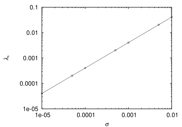
The total energy per unit translational Killing length decreases by the emission of gravitational radiation. The total value of the new -energy is initially equal to , while it finally becomes . The energy has been released by the gravitational radiation. The numerical results imply that for (see Fig.10). Accordingly the ratio of the emitted energy to the initial one depends on in the manner
| (56) |
The lighter the weight of the dust cylinder is, the larger the efficiency becomes. In zero-mass limit, the efficiency becomes unity. This seems to be paradoxical, but we should note that it is a non-trivial matter how to relate the present results with the asymptotically flat cases, e.g., the situation treated by Shapiro and Teukolsky[8]. From the point of view of the original -energy , the infinite amount of energy is released by the collapse of the dust cylinder; we can easily see that total value of the original -energy finally becomes
| (57) |
for any radial coordinate , whereas it is initially infinite.
7 Summary and Discussion
We constructed numerical solutions for the Einstein equations, which describe the collapse of an imploding hollow cylinder composed of dust with a requirement that the dust particles stay the symmetry axis after these reach there. A spacetime singularity forms at its symmetry axis. Although the rest mass density and the curvature polynomials blow up at the spacetime singularity, this spacetime singularity causes at most regular singular points in Einstein equations. Thus if appropriate boundary conditions are imposed, components of the metric tensor are everywhere finite. Then the causal future of the spacetime singularity exists and the resultant spacetime singularity is naked.
We also obtained an analytic solution which asymptotically well agrees with our numerical solutions. This asymptotic solution reveals that infinite amount of energy per unit translational Killing length is released to infinity by the gravitational radiation, and a conical singularity remains at the symmetry axis as a final product. Strictly speaking, this is a counterexample of the second type for the weak cosmic censorship conjecture. However, since this naked singularity is merely conical, it is not so serious.
It might be a surprising fact for some readers that the remnant naked singularity formed by gravitational collapse of a dust cylinder is weak. In Newtonian theory of gravity, collapse of a dust cylinder finally produces a gravitational potential which logarithmically diverges at its symmetry axis, and thus the singularity is strong in Tipler’s sense. The reason of this difference between Newtonian gravity and relativity is as follows. The Newtonian gravitational potential produced by a dust cylinder of radius is
| (58) |
where is an integration constant, and is the mass per unit length,
| (59) |
Usually, we assume that is conserved in the framework of Newtonian gravity. Then logarithmically diverges at when the dust cylinder becomes infinitesimally thin, i.e., . By contrast, the present prescription does not guarantee the constancy of , and require that vanishes finally. Thus, if the present prescription is adopted in the framework of Newtonian gravity, the Newtonian gravitational potential finally vanishes. This prescription seems to be unphysical from a point of view of the mass conservation in Newtonian theory. However, it is not so from a point of view of the -energy conservation in general relativity. Although the tidal force finally vanishes except on the symmetry axis, the -energy is condensed on the symmetry axis, and produces a conical singularity there, in the framework of general relativity. The present prescription requires that the equation of state changes from dust to something other than dust, and the Newtonian approximation is not applicable to this changed equation of state.
Here it might be useful to compare the present analysis with that of paper I. In paper I, we required that the dust particles pass through the symmetry axis after these reach there. In the resultant spacetime, almost all of geodesics are complete and thus this may not be a counterexample for the extended weak cosmic censorship conjecture, as mentioned in Sec.1. This example revealed that the gravity produced by the collapsed dust cylinder is too weak to confine the collisionless particles to the symmetry axis. In contrast, in the present prescription, matter is confined to the symmetry axis, but it is due to not the gravity, but the change of interactions between particles, or the change of the equation of state. It should be noted that this change in the equation of state is a result by requiring the smoothest behaviors of the metric components like as the Morgan’s null dust solution.
Finally, we note that, in order to complete an analysis to see whether a numerical model like as that of Shapiro and Teukolsky is a counterexample for the cosmic censorship conjecture, we need to specify the boundary conditions at the “spacetime singularity”. If we do not so, we can not know whether the “singularity” is really singular, or whether the cosmic censorship conjecture holds in a real singularity case. For this purpose, we need the knowledge of the global structure of the spacetime. In this sense, the analyses of paper I and the present paper are the first step of the attempt toward the numerical study of the weak cosmic censorship conjecture.
Acknowledgments
We are grateful to H. Ishihara and colleagues in the astrophysics and gravity group of Osaka City University for their useful and helpful discussion and criticism. This work is supported by the Grant-in-Aid for Scientific Research (No.16540264).
Appendix A Riemann tensor of self-similar gravitational waves
References
- [1] S. W. Hawking and G. F. R. Ellis, The large scale structure of space-time, (Cambridge University Press, Cambridge, 1973).
- [2] T. Harada and K. Nakao, Phys. Rev. D 70, 041501 (2004).
- [3] R. Penrose, Riv. Nuovo Cimento 1, 252 (1969).
- [4] A. Ori, Phys. Rev. Lett. 68, 2117 (1992).
- [5] L.M. Burko, Phys. Rev. Lett., 79, 4958 (1997).
- [6] M. Dafermos and I. Rodnianski, arXiv:gr-qc/0309115.
- [7] R.M. Wald, arXiv:gr-qc/9710068.
- [8] S. L. Shapiro and S. A. Teukolsky, Phys. Rev. Lett. 66 994 (1991).
- [9] K. S. Thorne, in Magic Without Magic; John Archibald Wheeler, edited by J. Klauder, (Frieman, San Francisco, 1972), p. 231.
- [10] S. A. Hayward, Class. Quantum Grav. 17, 1749 (2000).
- [11] T. A. Morgan, Gen. Rel. Grav. 4, 273 (1973).
- [12] F. Echeverria, Phys. Rev. D 47, 2271 (1993).
- [13] P. S. Letelier and A. Wang, Phys. Rev. D49, 5105 (1994).
- [14] T. Chiba, Prog. Theor. Phys. 95, 321 (1996).
- [15] B. C. Nolan, Phys. Rev. D 65, 104006 (2002).
- [16] K. Nakao, Y. Kurita, Y. Morisawa and T. Harada, Prog. Theor. Phys. 117, 75 (2007).
- [17] D. M. Eardley and L. Smarr, Phys. Rev. D 19, 2239 (1979).
- [18] D. Christodoulou, Commun. Math. Phys. 93, 171 (1984).
- [19] R. P. A. C. Newman, Class. Quantum Grav. 3, 527 (1986).
- [20] P. Joshi, Global Aspects in Gravitation and Cosmology (Oxford University Press, New York, 1993). References about the spherically symmetric cases are therein.
- [21] T. Harada, H. Iguchi and K. Nakao, Phys. Rev. D 58, 041502 (1998).
- [22] F. J. Tipler, Phys. Lett. 64A, 8 (1977).
- [23] C.J.S. Clarke, The Analysis of Space-Time Singularities (Cambridge University Press, 1993).
- [24] K. Lake, Phys. Rev. Lett. 68, 3129 (1992).
- [25] M. A. Melvin, Phys. Lett. 8, 65 (1964).
- [26] M. A. Melvin, Phys. Rev. 139, B225 (1965).
- [27] Y. Kurita and K. Nakao, Phys. Rev. D 73 064022 (2006).
- [28] A. Królak, J. Math. Phys. 28, 138 (1987).
- [29] W. Israel, Phys. Rev. D 15, 935 (1977).
- [30] R. Geroch and J. Traschen, Phys. Rev. D 36, 1017 (1987).
- [31] K. S. Thorne, Phys. Rev. 138, B251 (1965).
- [32] T. Harada, K. Nakao and B. Nolan, arXiv:0812.3462.