跳到论文正文
W Papers独立论文阅读器 arXiv:0905.3837 论文正文 计算阅读时间 · 0%
引用这篇论文根据当前论文元数据生成,正式投稿前建议核对。


License: arXiv.org perpetual non-exclusive license
arXiv:0905.3837v3 [math.OC] 01 Sep 2009

On the transport dimension of measuresThanks: This work is supported by an NSF grant DMS-0710714.

Qinglan Xia, Anna Vershynina Address: University of California at Davis
Department of Mathematics
Davis,CA,95616
Email address: qlxia@math.ucdavis.edu URL: http://math.ucdavis.edu/˜qlxia
Abstract.

In this article, we define the transport dimension of probability measures on ℝm\mathbb{R}^{m} using ramified optimal transportation theory. We show that the transport dimension of a probability measure is bounded above by the Minkowski dimension and below by the Hausdorff dimension of the measure. Moreover, we introduce a metric, called “the dimensional distance”, on the space of probability measures on ℝm\mathbb{R}^{m}. This metric gives a geometric meaning to the transport dimension: with respect to this metric, we show that the transport dimension of a probability measure equals to the distance from it to any finite atomic probability measure.

Key words and phrases: 
optimal transport path, ramified optimal transportation, fractal dimension of measures, transport dimension, irrigation dimension
2000 Mathematics Subject Classification
Primary 49Q20, 51F99; Secondary 28E05, 90B06

1. Introduction

The theory of ramified optimal transportation aims at finding an optimal transport path between two given probability measures. One of the measures is representing the source while the other is representing the target. A transport path is typically in the form of a tree-shaped branching structure. A natural question is: given a probability measure, is it possible to transport it to a Dirac mass via a finite cost transport path? The answer to this question crucially depends on the dimensional information of the given measure.

In [8], Devillanova and Solimini studied the irrigability dimension of measures using optimal transportation theory. For any given probability measure μ\mu on ℝm\mathbb{R}^{m}, the irrigability dimension of μ\mu is defined by

dimI(μ):=inf0≤α<1{11−α: if ​μ​ is ​α−irrigable}.\dim_{I}\left(\mu\right):=\inf_{0\leq\alpha<1}\left\{\frac{1}{1-\alpha}:\text{ if }\mu\text{ is }\alpha-\text{irrigable}\right\}.

The main theorem in [8] shows that

(1.1) max⁡{dimH(μ),1}≤dimI(μ)≤max⁡{1,dimM(μ)}\max\left\{\dim_{H}\left(\mu\right),1\right\}\leq\dim_{I}\left(\mu\right)\leq\max\left\{1,\dim_{M}\left(\mu\right)\right\}

where dimH(μ)\dim_{H}\left(\mu\right) (or dimM(μ)\dim_{M}\left(\mu\right)) denotes the infimum of the Hausdorff dimension (or the Minkowski dimension, respectively) of sets that μ\mu is concentrated on. By definition, the irrigability dimension dimI(μ)\dim_{I}\left(\mu\right) of a measure μ\mu must be larger or equal to 11 as the parameter α\alpha is in the range of [0,1)[0,1).

In this article, we aim at removing the maximum constraint from (1.1) by using a different approach of ramified optimal transportation (i.e. using optimal transport paths), and also allowing the parameter α\alpha to be negative. This generalization allows us to consider measures which have fractal dimensions (e.g. the Cantor measure) less than 11. We introduce an analogous concept called “the transport dimension of μ\mu”, and show in theorem 3.5.2 that

dimH(μ)≤dimT(μ)≤dimM(μ)\dim_{H}\left(\mu\right)\leq\dim_{T}\left(\mu\right)\leq\dim_{M}\left(\mu\right)

with a slight modification of the definition of dimM(μ)\dim_{M}\left(\mu\right). The major difference between dimI(μ)\dim_{I}\left(\mu\right) and dimT(μ)\dim_{T}\left(\mu\right) is that dimT(μ)\dim_{T}\left(\mu\right) is allowed to be less than 1. For instance, for the Cantor measure, we show that dimT(μ)\dim_{T}\left(\mu\right) is ln⁡2ln⁡3\frac{\ln 2}{\ln 3} which is exactly the dimension of the Cantor set.

Moreover, we find a geometric meaning to the transport dimension by introducing a new metric, called “the dimensional distance”, on the space of equivalent classes of probability measures. With respect to this metric, the distance of any probability measure to a Dirac mass (or any atomic probability measure) equals to the transport dimension of the measure. In other words, the transport dimension of a measure quantitatively describes how far the measure is from being an atomic measure.

We refer to the book [3] as well as references there for a modern account of optimal transportation with branching structures. In particular, a partial list of most relevant works is listed in the reference: [1],[2],[4],[6],[7],[9],[10],[11],[12],[14],[15],[16], [18],[19] and of course [8].

Organization of the paper. We first recall some basic concepts about optimal transport paths in section 2 with some necessary modifications. We show that for any α∈(−∞,1)\alpha\in\left(-\infty,1\right), there exists a metric dαd_{\alpha} on the space 𝒜⁡(ℝm)\mathcal{A}\left(\mathbb{R}^{m}\right) of atomic probability measures. Then, we consider the metric completion 𝒫α​(ℝm)\mathcal{P}_{\alpha}\left(\mathbb{R}^{m}\right) of 𝒜⁡(ℝm)\mathcal{A}\left(\mathbb{R}^{m}\right) with respect to each dαd_{\alpha}. We show that when a probability measure is concentrated on a set whose box dimension is less than 11−α\frac{1}{1-\alpha}, then the measure belongs to 𝒫α\mathcal{P}_{\alpha}. After that, we begin to consider the transport dimension of measures in section 3 with some comparison with other dimension of measures. In particular, we show that the transport dimension of a measure is bounded above by its Minkowski dimension and bounded below by its Hausdorff dimension. We also show the transport dimension of the Cantor measure is ln⁡2ln⁡3\frac{\ln 2}{\ln 3}. In section 4, we consider the dimensional distance between probability measures. The main result there says that the transport dimension of a probability measure is given by the distance of the measure to any atomic probability measure with respect to the dimensional distance.

2. The dαd_{\alpha} metric on probability measures for α∈(−∞,1)\alpha\in\left(-\infty,1\right)

2.1. Transport paths between atomic measures

We first recall some basic concepts about transport paths between measures of equal total mass as studied in [11], with some necessary modifications.

Recall that a (finite) atomic measure on ℝm\mathbb{R}^{m} is in the form of

(2.1) 𝐚=∑i=1kmi​δxi\mathbf{a=}\sum_{i=1}^{k}m_{i}\delta_{x_{i}}

with distinct points xi∈ℝmx_{i}\in\mathbb{R}^{m}, and positive real numbers mi,m_{i}, where δx\delta_{x} denotes the Dirac mass located at the point xx. The measure 𝐚\mathbf{a} is a probability measure if its mass ||𝐚||:=∑i=1kmi=1\left|\left|\mathbf{a}\right|\right|:=\sum_{i=1}^{k}m_{i}=1. Let 𝒜⁡(ℝm)\mathcal{A}(\mathbb{R}^{m}) be the space of all atomic probability measures on ℝm\mathbb{R}^{m}.

Definition 2.1.1.

Given two atomic measures

(2.2) 𝐚=∑i=1kmi​δxi​ and ​𝐛=∑j=1ℓnj​δyj\mathbf{a}=\sum_{i=1}^{k}m_{i}\delta_{x_{i}}\text{ and }\mathbf{b}=\sum_{j=1}^{\ell}n_{j}\delta_{y_{j}}

in ℝm\mathbb{R}^{m}of equal mass, a transport path from 𝐚\mathbf{a} to 𝐛\mathbf{b} is a weighted directed graph GG consisting of a vertex set V⁡(G)V(G), a directed edge set E⁡(G)E(G) and a weight function w:E⁡(G)→(0,+∞)w:E(G)\rightarrow(0,+\infty) such that {x1,x2,…,xk}∪{y1,y2,…,yℓ}⊂V⁡(G)\{x_{1},x_{2},...,x_{k}\}\cup\{y_{1},y_{2},...,y_{\ell}\}\subset V(G) and for any vertex v∈V⁡(G)v\in V(G),

(2.3) ∑e∈E⁡(G),e−=vw⁡(e)=∑e∈E⁡(G),e+=vw⁡(e)+{mi, if ​v=xi​ for some ​i=1,…,k−nj, if ​v=yj​ for some ​j=1,…,ℓ0, otherwise \sum_{e\in E(G),e^{-}=v}w(e)=\sum_{e\in E(G),e^{+}=v}w(e)+\left\{\begin{array}[]{c}m_{i},\text{\ if }v=x_{i}\text{\ for some }i=1,...,k\\ -n_{j},\text{\ if }v=y_{j}\text{\ for some }j=1,...,\ell\\ 0,\text{\ otherwise }\end{array}\right.

where e−e^{-} and e+e^{+} denotes the starting and ending endpoints of each edge e∈E⁡(G)e\in E(G).

Note that the balanced equation (2.3) simply means the conservation of mass at each vertex. In terms of polyhedral chains, we simply have ∂G=b−a\partial G=b-a.

For any two atomic measures 𝐚\mathbf{a} and 𝐛\mathbf{b} on ℝm\mathbb{R}^{m} of equal total mass, let

P​a​t​h​(𝐚,𝐛)Path(\mathbf{a},\mathbf{b})

be the space of all transport paths from 𝐚\mathbf{a} to 𝐛\mathbf{b}. It is easy to see to that P​a​t​h​(𝐚,𝐛)Path\left(\mathbf{a},\mathbf{b}\right) is always nonempty.

Definition 2.1.2.

For any α≤1\alpha\leq 1 and any transport path G∈Path​(𝐚,𝐛)G\in\text{Path}(\mathbf{a},\mathbf{b}), we define

𝐌α​(G):=∑e∈E⁡(G)w​(e)α​length​(e).\mathbf{M}_{\alpha}(G):=\sum_{e\in E(G)}w(e)^{\alpha}\text{length}(e).

We now consider the following ramified optimal transport problem:

Problem 1.

Given two atomic measures 𝐚\mathbf{a} and 𝐛\mathbf{b} of equal mass on ℝm\mathbb{R}^{m} and −∞<α<1-\infty<\alpha<1, find a minimizer of

𝐌α​(G)\mathbf{M}_{\alpha}(G)

among all transport paths G∈P​a​t​h​(𝐚,𝐛)G\in Path\left(\mathbf{a},\mathbf{b}\right).

An 𝐌α\mathbf{M}_{\alpha} minimizer in P​a​t​h​(𝐚,𝐛)Path(\mathbf{a},\mathbf{b}) is called an α−\alpha-optimal transport path from 𝐚\mathbf{a} to 𝐛\mathbf{b}.

Note that in [11, Definition 2.2], we only allow that 0≤α≤10\leq\alpha\leq 1. But now, for the purpose of studying fractal dimension of measures in this article, we also allow negative α\alpha. Negative α\alpha also corresponds to many transport problems in reality. For instance, the “cost” (i.e. risk here) for a baby to go back home from his preschool by himself is much higher than the one for an adult. This is why babies need to be picked up by adults. In this example, the cost of transporting a higher density mass (i.e. an adult) is less than the cost of transporting a lower density mass (i.e. a baby). Negative α\alpha is used for such phenomenon. Another application of ramified optimal transportation with negative α\alpha may be found in [17].

Definition 2.1.3.

For any α≤1\alpha\leq 1, we define

dα​(𝐚,𝐛)=inf{𝐌α​(G):G∈P​a​t​h​(𝐚,𝐛)}d_{\alpha}\left(\mathbf{a},\mathbf{b}\right)=\inf\left\{\mathbf{M}_{\alpha}\left(G\right):G\in Path\left(\mathbf{a},\mathbf{b}\right)\right\}

for any 𝐚,𝐛∈𝒜⁡(ℝm)\mathbf{a},\mathbf{b\in}\mathcal{A}(\mathbb{R}^{m}).

Remark 2.1.4.

If 𝐚~\mathbf{\tilde{a}} and 𝐛~\mathbf{\tilde{b}} are two atomic measures of equal total mass Λ\Lambda, and let 𝐚=1Λ​𝐚~\mathbf{a}=\frac{1}{\Lambda}\mathbf{\tilde{a}} and 𝐛=1Λ​𝐛~\mathbf{b}=\frac{1}{\Lambda}\mathbf{\tilde{b}} be the normalization of 𝐚~\mathbf{\tilde{a}} and 𝐛~\mathbf{\tilde{b}}. Then, we set

dα​(𝐚~,𝐛~)=Λα​dα​(𝐚,𝐛).d_{\alpha}\left(\mathbf{\tilde{a}},\mathbf{\tilde{b}}\right)=\Lambda^{\alpha}d_{\alpha}\left(\mathbf{a},\mathbf{b}\right).

2.2. Behavior of transport paths for a negative α\alpha

The behavior of an α−\alpha-optimal transport path is quite different for a negative α\alpha and a nonnegative α\alpha. For instance, in [11, proposition 2.1], we shown that for nonnegative α\alpha, an α\alpha-optimal transport path contains no cycles. On the hand, from the following example 2.2.1, an α−\alpha-optimal transport path may prefer to have a cycle when α\alpha is negative.

Example 2.2.1.

Let 𝐚=δ0\mathbf{a=\delta}_{0}, 𝐛=0.8​δ0+0.2​δ1∈𝒜⁡(ℝ)\mathbf{b=}0.8\delta_{0}+0.2\delta_{1}\in\mathcal{A}(\mathbb{R}), then we may construct two transport paths from 𝐚\mathbf{a} to 𝐛\mathbf{b}. One contains a cycle while the other does not.

Refer to caption
Figure 1. For α<0\alpha<0, an optimal transport path may contain a cycle

The first transport path G1G_{1} consists of only one directed edge from 00 to 11 with a weight 0.20.2. The second transport path G2G_{2} consists of two directed edges: one from 00 to 11 with a weight 11 and the other from 11 to 00 with a weight 0.80.8. Then, when α<−12\alpha<-\frac{1}{2}, we have

𝐌α​(G2)𝐌α​(G1)=1α+0.8α0.2α≤0.8α+0.8α0.2α=21+2​α<1.\frac{\mathbf{M}_{\alpha}\left(G_{2}\right)}{\mathbf{M}_{\alpha}\left(G_{1}\right)}=\frac{1^{\alpha}+0.8^{\alpha}}{0.2^{\alpha}}\leq\frac{0.8^{\alpha}+0.8^{\alpha}}{0.2^{\alpha}}=2^{1+2\alpha}<1.

Thus, 𝐌α​(G2)<𝐌α​(G1)\mathbf{M}_{\alpha}\left(G_{2}\right)<\mathbf{M}_{\alpha}\left(G_{1}\right). i.e. a path containing a cycle may have less 𝐌α\mathbf{M}_{\alpha} cost.

A transport path may also contain another type of cycles, which are unpleasant for our study.

Refer to caption
Figure 2. An unpleasant cycle appeared in a transport path
Example 2.2.2.

From definition, it is possible for a transport path to contain another type of directed cycles which are similar to the one appearing in figure 2. Using this directed cycle, the original weight “ 0.50.5” of the edge in the example may either be repeatedly counted or be combined with some mass from unknown sources (which may have nothing to do with 𝐚\mathbf{a} or 𝐛\mathbf{b}), and lead to a new very high weight “ n+0.5n+0.5” in the end. When α\alpha is negative and nn is large, (n+0.5)α(n+0.5)^{\alpha} may become a very small positive number, much less than 0.5α0.5^{\alpha}. Thus, for negative α\alpha, one may significantly decrease the 𝐌α\mathbf{M}_{\alpha} cost of a transport path by repeatedly adding a directed cycle of this type with a very large weighting constant nn. Since the value nαn^{\alpha} approaches zero as nn approaches to infinity when α<0\alpha<0, allowing such kind of directed cycles in the family P​a​t​h​(𝐚,𝐛)Path\left(\mathbf{a},\mathbf{b}\right) may eventually lead to an unpleasant result: dα​(𝐚,𝐛)=0d_{\alpha}\left(\mathbf{a},\mathbf{b}\right)=0 for 𝐚≠𝐛\mathbf{a}\neq\mathbf{b}.

The cycle in example 2.2.1 is desirable while the cycle in example 2.2.2 is not what we want. To overcome this conflict of interests, we adopt the following convention on the definition of transport paths when α\alpha is negative.

Convention 2.2.3.

For any vertex v∈V⁡(G)v\in V\left(G\right) of a transport path GG, if there exists a list of vertices {v1,v2,⋯,vn}\left\{v_{1},v_{2,}\cdots,v_{n}\right\} such that v1=vn=vv_{1}=v_{n}=v and [vi,vi+1]\left[v_{i},v_{i+1}\right] is a directed edge in E⁡(G)E\left(G\right) with a positive edge length for each i=1,2,⋯,n−1i=1,2,\cdots,n-1, then we will view vnv_{n} as a different copy of the point vv. In other words, vnv_{n} and vv are two different vertices in V⁡(G)V\left(G\right) and thus the balance equation (2.3) must be separately hold at each of them.

Using this convention, one cannot “combine” the weights of edges from the vertex vnv_{n} with weights of edges from the different vertex v1v_{1}. So the weight of an edge cannot be repeatedly counted leading to a very large number, and must be bounded above by the total mass of 𝐚\mathbf{a}. As a result, the convention implies two consequences: a transport path will no longer contain a directed cycle in the type of example 2.2.2. Moreover, we have a universal upper bound (i.e. the total mass of the source) on the weight of each edge:

(2.4) w⁡(e)≤||𝐚||w\left(e\right)\leq\left|\left|\mathbf{a}\right|\right|

for each edge ee of a transport path GG from 𝐚\mathbf{a} to 𝐛\mathbf{b}. In particular, if 𝐚\mathbf{a} is a probability measure, then w⁡(e)≤1w\left(e\right)\leq 1.

For nonnegative α\alpha, since an α−\alpha-optimal transport path contains no cycles (as shown in [11, proposition 2.1]), there is no need to adopt this convention then.

Many properties about transport paths have been studied in [11],[12],[13], [14],[16] and [3] when 0≤α<10\leq\alpha<1. For instance, we showed in [11, theorem 5.1] that (𝒜⁡(ℝm),dα)\left(\mathcal{A}(\mathbb{R}^{m}),d_{\alpha}\right) is a geodesic space, and it is indeed a metric induced by a quasimetric (see [16]). As the main purpose of this article is studying dimensions of measures, we will leave the study of properties of optimal transport paths in the situation of α<0\alpha<0 to a later article. Currently, we only need to show that dαd_{\alpha} is still a metric on 𝒜⁡(ℝm)\mathcal{A}(\mathbb{R}^{m}) when α<0\alpha<0.

2.3. The dαd_{\alpha} metric when α<0\alpha<0

We denote S⁡(p,r)S\left(p,r\right) (and B¯​(p,r)\bar{B}\left(p,r\right), respectively) to be the sphere (and the closed ball, respectively) centered at p∈ℝmp\in\mathbb{R}^{m} of radius r>0r>0. Note that for any transport path GG, the restriction of GG on any closed ball B¯​(p,r0)\bar{B}\left(p,r_{0}\right) gives another transport path G|B¯​(p,r0)G|_{\bar{B}\left(p,r_{0}\right)}.

Lemma 2.3.1.

Suppose 𝐚\mathbf{a} and 𝐛\mathbf{b} are two atomic measures on ℝm\mathbb{R}^{m} of equal total mass, and GG is a transport path from 𝐚\mathbf{a} to 𝐛\mathbf{b}. If the intersection of G∩S⁡(p,r)G\cap S\left(p,r\right) as sets is nonempty for almost all r∈[0,r0]r\in\left[0,r_{0}\right] for some r0>0r_{0}>0, then for any α<0\alpha<0, we have

𝐌α​(G|B¯​(p,r0))≥Λα​r0,\mathbf{M}_{\alpha}\left(G|_{\bar{B}\left(p,r_{0}\right)}\right)\geq\Lambda^{\alpha}r_{0},

where Λ\Lambda is any upper bound of the weights of edges in G|B¯​(p,r0)G|_{\bar{B}\left(p,r_{0}\right)}.

Proof.

For any r>0r>0, let

𝐄r:={e∈E⁡(G):e∩S⁡(p,r)≠∅}\mathbf{E}_{r}:=\left\{e\in E\left(G\right):e\cap S\left(p,r\right)\neq\emptyset\right\}

be the family of all edges of GG that intersects with the sphere S⁡(p,r)S\left(p,r\right). By assumption, 𝐄r\mathbf{E}_{r} is nonempty for almost all r∈[0,r0]r\in\left[0,r_{0}\right].

Let LL be any fixed ray with endpoint pp, and let P:ℝm→LP:\mathbb{R}^{m}\rightarrow L be the projection that maps any point x∈ℝmx\in\mathbb{R}^{m} to the point P⁡(x)∈LP\left(x\right)\in L with |P⁡(x)−p|=|x−p|\left|P\left(x\right)-p\right|=\left|x-p\right|. Note that for any edge e∈E⁡(G)e\in E\left(G\right), under the projection PP, the length of the segment P⁡(e)P\left(e\right) is no more than the length of ee. Therefore,

𝐌α​(G|B¯​(p,r0))\displaystyle\mathbf{M}_{\alpha}(G|_{\bar{B}\left(p,r_{0}\right)}) =\displaystyle= ∑e∈E⁡(G∣B⁡(p,r0))[w⁡(e)]α​length​(e)\displaystyle\sum_{e\in E\left(G\mid B\left(p,r_{0}\right)\right)}\left[w(e)\right]^{\alpha}\text{length}(e)
≥\displaystyle\geq ∑e∈E⁡(G∣B⁡(p,r0))[w⁡(e)]α​length​(P⁡(e))\displaystyle\sum_{e\in E\left(G\mid B\left(p,r_{0}\right)\right)}\left[w(e)\right]^{\alpha}\text{length}(P\left(e\right))
=\displaystyle= ∫0r0∑e∈E⁡(G∣B⁡(p,r0))[w⁡(e)]α​χP⁡(e)​(r)​𝑑r\displaystyle\int_{0}^{r_{0}}\sum_{e\in E\left(G\mid B\left(p,r_{0}\right)\right)}\left[w(e)\right]^{\alpha}\chi_{P\left(e\right)}\left(r\right)dr
=\displaystyle= ∫0r0∑e∈𝐄r[w⁡(e)]α​𝑑r.\displaystyle\int_{0}^{r_{0}}\sum_{e\in\mathbf{E}_{r}}\left[w(e)\right]^{\alpha}dr.

where in the second equality χA\chi_{A} denotes the characteristic function on a set AA. So, we have shown that

(2.5) 𝐌α​(G|B¯​(p,r0))≥∫0r0∑e∈𝐄r[w⁡(e)]α​𝑑r.\mathbf{M}_{\alpha}(G|_{\bar{B}\left(p,r_{0}\right)})\geq\int_{0}^{r_{0}}\sum_{e\in\mathbf{E}_{r}}\left[w(e)\right]^{\alpha}dr.

Now, since w⁡(e)≤Λw\left(e\right)\leq\Lambda for any e∈𝐄r≠∅e\in\mathbf{E}_{r}\neq\emptyset and α<0\alpha<0, (2.5) yields

𝐌α​(G|B¯​(p,r0))≥∫0r0maxe∈𝐄r⁡[w⁡(e)]α​𝑑r≥∫0r0Λα​𝑑r=Λα​r0.\mathbf{M}_{\alpha}(G|_{\bar{B}\left(p,r_{0}\right)})\geq\int_{0}^{r_{0}}\max_{e\in\mathbf{E}_{r}}\left[w(e)\right]^{\alpha}dr\geq\int_{0}^{r_{0}}\Lambda^{\alpha}dr=\Lambda^{\alpha}r_{0}.

∎

Corollary 2.3.2.

Suppose α≤0\alpha\leq 0 and p∈ℝmp\in\mathbb{R}^{m}. Then, for any atomic measure

𝐚=∑i=1kmi​δxi\mathbf{a=}\sum_{i=1}^{k}m_{i}\delta_{x_{i}}

on ℝm\mathbb{R}^{m} with mass ||𝐚||:=∑i=1kmi>0\left|\left|\mathbf{a}\right|\right|:=\sum_{i=1}^{k}m_{i}>0 and any G∈P​a​t​h​(𝐚,||𝐚||​δp)G\in Path\left(\mathbf{a,\left|\left|\mathbf{a}\right|\right|\delta}_{p}\right) we have

𝐌α​(G)≥||𝐚||α​|p−xi|\mathbf{M}_{\alpha}\left(G\right)\geq\left|\left|\mathbf{a}\right|\right|^{\alpha}\left|p-x_{i}\right|

for each i=1,2,⋯,ki=1,2,\cdots,k.

Proof.

By (2.4), w⁡(e)≤||𝐚||w\left(e\right)\leq\left|\left|\mathbf{a}\right|\right| for any edge e∈E⁡(G)e\in E\left(G\right). Then, the result follows from lemma 2.3.1 by setting r0=max1≤i≤k⁡{|p−xi|}r_{0}=\max_{1\leq i\leq k}\left\{\left|p-x_{i}\right|\right\} and Λ=\Lambda= ||𝐚||\left|\left|\mathbf{a}\right|\right|. ∎

The inequality (2.5) also gives a lower bound estimate for positive α\alpha.

Corollary 2.3.3.

Suppose 0≤α<10\leq\alpha<1. For any 𝐚∈𝒜⁡(ℝm)\mathbf{a\in}\mathcal{A}(\mathbb{R}^{m}) in the form of (2.1), p∈ℝmp\in\mathbb{R}^{m} and r0>0r_{0}>0, we have

(2.6) [∑d⁡(p,xi)>r0mi]α≤dα​(𝐚,δp)r0.\left[\sum_{d\left(p,x_{i}\right)>r_{0}}m_{i}\right]^{\alpha}\leq\frac{d_{\alpha}(\mathbf{a},\delta_{p})}{r_{0}}.
Proof.

Let λ=∑d⁡(p,xi)>r0mi\lambda=\sum_{d\left(p,x_{i}\right)>r_{0}}m_{i}. Let GG be any transport path from 𝐚\mathbf{a} to δp\delta_{p}. Then, for any 0<r≤r00<r\leq r_{0}, we have

∑e∈𝐄rw⁡(e)≥λ.\sum_{e\in\mathbf{E}_{r}}w(e)\geq\lambda.

By the inequality (2.5), since the function f⁡(x)=xαf\left(x\right)=x^{\alpha} is concave on [0,1]\left[0,1\right] when 0≤α<10\leq\alpha<1, we have

𝐌α​(G|B¯​(p,r0))\displaystyle\mathbf{M}_{\alpha}(G|_{\bar{B}\left(p,r_{0}\right)}) ≥\displaystyle\geq ∫0r0∑e∈𝐄r[w⁡(e)]α​𝑑r\displaystyle\int_{0}^{r_{0}}\sum_{e\in\mathbf{E}_{r}}\left[w(e)\right]^{\alpha}dr
≥\displaystyle\geq ∫0r0[∑e∈𝐄rw⁡(e)]α​𝑑r≥∫0r0λα​𝑑r=λα​r0​.\displaystyle\int_{0}^{r_{0}}\left[\sum_{e\in\mathbf{E}_{r}}w(e)\right]^{\alpha}dr\geq\int_{0}^{r_{0}}\lambda^{\alpha}dr=\lambda^{\alpha}r_{0}\text{.}

Therefore, we have (2.6). ∎

Proposition 2.3.4.

dαd_{\alpha} is a metric on 𝒜⁡(ℝm)\mathcal{A}(\mathbb{R}^{m}).

Proof.

Obviously, we only need to consider the case α<0\alpha<0. In this case, it is clear that dαd_{\alpha} is nonnegative and symmetric. Now, for any 𝐚,𝐛,𝐜∈𝒜⁡(ℝm)\mathbf{a},\mathbf{b,c\in}\mathcal{A}(\mathbb{R}^{m}) and any path G1∈P​a​t​h​(𝐚,𝐛)G_{1}\in Path\left(\mathbf{a},\mathbf{b}\right) and G2∈P​a​t​h​(𝐛,𝐜)G_{2}\in Path\left(\mathbf{b},\mathbf{c}\right), let G3G_{3} be the disjoint union of the directed weighted graphs G1G_{1} and G2G_{2}. That is,

V⁡(G3)=(V⁡(G1)∖V⁡(𝐛))​∐(V⁡(G2)∖V⁡(𝐛))​∐V⁡(𝐛)V\left(G_{3}\right)=\left(V\left(G_{1}\right)\setminus V(\mathbf{b})\right)\coprod\left(V\left(G_{2}\right)\setminus V(\mathbf{b})\right)\coprod V(\mathbf{b})

and E⁡(G3)=E⁡(G1)​∐E⁡(G2)E\left(G_{3}\right)=E\left(G_{1}\right)\coprod E\left(G_{2}\right), where the symbol ∐\coprod denotes the disjoint union of sets, and V⁡(𝐛)V(\mathbf{b}) denotes the vertex set (i.e. the support) of the measure 𝐛\mathbf{b}. Then, by using the convention 2.2.3, G3G_{3} is a transport path from 𝐚\mathbf{a} to 𝐜\mathbf{c} with

𝐌α​(G3)=𝐌α​(G1)+𝐌α​(G2).\mathbf{M}_{\alpha}\left(G_{3}\right)=\mathbf{M}_{\alpha}\left(G_{1}\right)+\mathbf{M}_{\alpha}\left(G_{2}\right).

Thus, by taking infimum, we have the triangle inequality

dα​(𝐚,𝐜)≤dα​(𝐚,𝐛)+dα​(𝐛,𝐜)​.d_{\alpha}\left(\mathbf{a},\mathbf{c}\right)\leq d_{\alpha}\left(\mathbf{a},\mathbf{b}\right)+d_{\alpha}\left(\mathbf{b},\mathbf{c}\right)\text{.}

Now, we only need to check that if 𝐚≠𝐛\mathbf{a}\neq\mathbf{b}, then dα​(𝐚,𝐛)>0d_{\alpha}\left(\mathbf{a},\mathbf{b}\right)>0. We may assume that 𝐚\mathbf{a} and 𝐛\mathbf{b} are in the forms of (2.2). If the supports of 𝐚\mathbf{a} and 𝐛\mathbf{b} are different, i.e. {y1,y2,⋯,yl}≠{x1,x2,⋯,xk}\left\{y_{1},y_{2},\cdots,y_{l}\right\}\neq\left\{x_{1},x_{2},\cdots,x_{k}\right\} as sets, we may assume that y1∉{x1,x2,⋯,xk}y_{1}\notin\left\{x_{1},x_{2},\cdots,x_{k}\right\}. In this case, we set p=y1p=y_{1} and

r0:=min{|p−xi|:i=1,2,⋯,k}>0.r_{0}:=\min\left\{\left|p-x_{i}\right|:i=1,2,\cdots,k\right\}>0\text{.}

If {x1,x2,⋯,xk}={y1,y2,⋯,yl}\left\{x_{1},x_{2},\cdots,x_{k}\right\}=\left\{y_{1},y_{2},\cdots,y_{l}\right\} as sets, then we may assume

𝐚=∑i=1kmi​δxi​ and ​𝐛=∑i=1kni​δxi\mathbf{a}=\sum_{i=1}^{k}m_{i}\delta_{x_{i}}\text{ and }\mathbf{b}=\sum_{i=1}^{k}n_{i}\delta_{x_{i}}

and m1≠n1m_{1}\neq n_{1}. In this case, we set p=x1p=x_{1} and let

r0:=min{|p−xi|:mi≠ni, i=2,⋯,k}>0.r_{0}:=\min\left\{\left|p-x_{i}\right|:m_{i}\neq n_{i}\text{, }i=2,\cdots,k\right\}>0\text{.}

In any of these two cases, for any transport path GG from 𝐚\mathbf{a} to 𝐛\mathbf{b}, the intersection of GG with the sphere S⁡(p,r)S\left(p,r\right) is nonempty for any 0<r<r00<r<r_{0}. By lemma 2.3.1,

𝐌α​(G)≥r0\mathbf{M}_{\alpha}\left(G\right)\geq r_{0}

since w⁡(e)≤1w\left(e\right)\leq 1 for any edge e∈E⁡(G)e\in E\left(G\right). Therefore,

dα​(𝐚,𝐛)≥r0>0​.d_{\alpha}\left(\mathbf{a},\mathbf{b}\right)\geq r_{0}>0\text{.}

∎

2.3.1. The completion of 𝒜⁡(ℝm)\mathcal{A}\left(\mathbb{R}^{m}\right) with respect to dαd_{\alpha}

Definition 2.3.5.

For any α∈(−∞,1]\alpha\in(-\infty,1], let 𝒫α​(ℝm)\mathcal{P}_{\alpha}(\mathbb{R}^{m}) be the completion of the metric space 𝒜⁡(ℝm)\mathcal{A}(\mathbb{R}^{m}) with respect to the metric dαd_{\alpha}.

We will simply write 𝒫α​(ℝm)\mathcal{P}_{\alpha}(\mathbb{R}^{m}) as 𝒫α\mathcal{P}_{\alpha}.

Note that when α=1\alpha=1, the metric d1d_{1} is the usual Monge’s distance on 𝒜⁡(ℝm)\mathcal{A}(\mathbb{R}^{m}) and 𝒫1\mathcal{P}_{1} is the space 𝒫\mathcal{P} of all probability measures on ℝm\mathbb{R}^{m}. Now, the following lemma implies that each element in 𝒫α\mathcal{P}_{\alpha} can be viewed as a probability measure on ℝm\mathbb{R}^{m}.

Lemma 2.3.6.

If β<α\beta<\alpha, then 𝒫β​(ℝm)⊆𝒫α​(ℝm)\mathcal{P}_{\beta}(\mathbb{R}^{m})\subseteq\mathcal{P}_{\alpha}(\mathbb{R}^{m}), and for all μ,ν\mu,\nu in 𝒫β​(ℝm)\mathcal{P}_{\beta}(\mathbb{R}^{m}) we have dβ​(μ,ν)≥dα​(μ,ν)d_{\beta}(\mu,\nu)\geq d_{\alpha}(\mu,\nu).

Proof.

Note that for any path GG between any two probability measures 𝐚\mathbf{a} and 𝐛\mathbf{b} in 𝒜⁡(ℝm)\mathcal{A}(\mathbb{R}^{m}) we have

𝐌α​(G)=∑e∈E⁡(G)w​(e)α​length​(e)≤∑e∈E⁡(G)w​(e)β​length​(e)=𝐌β​(G).\mathbf{M}_{\alpha}(G)=\sum_{e\in E(G)}w(e)^{\alpha}\text{length}(e)\leq\sum_{e\in E(G)}w(e)^{\beta}\text{length}(e)=\mathbf{M}_{\beta}(G).

This is because w⁡(e)≤1w(e)\leq 1 for any e∈E⁡(G)e\in E(G). Hence

dα​(𝐚,𝐛)\displaystyle d_{\alpha}(\mathbf{a},\mathbf{b}) =\displaystyle= inf{𝐌α​(G):G∈Path​(𝐚,𝐛)}\displaystyle\inf\{\mathbf{M}_{\alpha}(G):G\in\text{Path}(\mathbf{a},\mathbf{b})\}
≤\displaystyle\leq inf{𝐌β​(G):G∈Path​(𝐚,𝐛)}=dβ​(𝐚,𝐛).\displaystyle\inf\{\mathbf{M}_{\beta}(G):G\in\text{Path}(\mathbf{a},\mathbf{b})\}=d_{\beta}(\mathbf{a},\mathbf{b}).

Therefore, any Cauchy sequence {𝐚n}\left\{\mathbf{a}_{n}\right\} in 𝒜⁡(ℝm)\mathcal{A}(\mathbb{R}^{m}) with respect to the metric dβd_{\beta} is also a Cauchy sequence with respect to dαd_{\alpha}. Thus, 𝒫β​(ℝm)⊆𝒫α​(ℝm)\mathcal{P}_{\beta}(\mathbb{R}^{m})\subseteq\mathcal{P}_{\alpha}(\mathbb{R}^{m}) with

dα​(μ,ν)≤dβ​(μ,ν)d_{\alpha}(\mu,\nu)\leq d_{\beta}(\mu,\nu)

for any μ,ν\mu,\nu in 𝒫β​(ℝm)\mathcal{P}_{\beta}(\mathbb{R}^{m}). ∎

As discussed in [8] the Minkowski-Bouligand dimension, also known as box-counting dimension of a set AA is given by

(2.7) dimb​o​x(A)\displaystyle\dim_{box}(A) =\displaystyle= inf{β>0:A can be covered by Cβδ−β balls of\displaystyle\inf\{\beta>0:A\text{ can be covered by }C_{\beta}\delta^{-\beta}\text{ balls of }
radius δ for all δ less than 1 and some constant Cβ}.\displaystyle\text{radius }\delta\text{ for all }\delta\text{ less than }1\text{ and some constant }C_{\beta}\}.

A positive Borel measure μ\mu on ℝm\mathbb{R}^{m} is said to be concentrated on a Borel set AA if μ⁡(ℝm∖A)=0\mu(\mathbb{R}^{m}\setminus A)=0.

Theorem 2.3.7.

Suppose μ\mu is a probability measure concentrated on a subset AA of ℝm\mathbb{R}^{m} with dimb​o​x(A)<11−α\dim_{box}(A)<\frac{1}{1-\alpha} for some 0≤α<10\leq\alpha<1, then μ∈𝒫α\mu\in\mathcal{P}_{\alpha}.

Proof.

Since dimb​o​x(A)<11−α\dim_{box}(A)<\frac{1}{1-\alpha}, we may fix a constant β\beta such that dimb​o​x(A)<β<11−α\dim_{box}(A)<\beta<\frac{1}{1-\alpha}. By (2.7), for every n∈ℕn\in\mathbb{N}, the set AA can be covered by balls {B⁡(xi(n),12n)}i=1Nn\left\{B\left(x_{i}^{\left(n\right)},\frac{1}{2^{n}}\right)\right\}_{i=1}^{N_{n}} of radius 12n\frac{1}{2^{n}} centering at xi(n)x_{i}^{\left(n\right)}, where the number NnN_{n} of balls of radius 12n\frac{1}{2^{n}} is bounded above by Cβ​(12n)−βC_{\beta}\left(\frac{1}{2^{n}}\right)^{-\beta} for some constant CβC_{\beta}. Using Vitali’s covering theorem (see for instance, [5, section 1.5.1]) we may assume that the balls {B⁡(xi(n),15⋅2n)}i=1Nn\left\{B\left(x_{i}^{\left(n\right)},\frac{1}{5\cdot 2^{n}}\right)\right\}_{i=1}^{N_{n}} are disjoint. For each ball B⁡(xi(n),12n)B\left(x_{i}^{\left(n\right)},\frac{1}{2^{n}}\right), let

Φi(n)={xj(n−1):B⁡(xi(n),12n)∩B⁡(xj(n−1),12n−1)≠∅}\Phi_{i}^{\left(n\right)}=\left\{x_{j}^{\left(n-1\right)}:B\left(x_{i}^{\left(n\right)},\frac{1}{2^{n}}\right)\cap B\left(x_{j}^{\left(n-1\right)},\frac{1}{2^{n-1}}\right)\neq\emptyset\right\}

be the set of centers of all balls in the preceding cover that intersects with B⁡(xi(n),12n)B\left(x_{i}^{\left(n\right)},\frac{1}{2^{n}}\right). Then one can easily check that the cardinality ki(n)k_{i}^{\left(n\right)} of Φi(n)\Phi_{i}^{\left(n\right)} is less than (172)m\left(\frac{17}{2}\right)^{m}.

Using these family of covers, we construct a Cauchy sequence {𝐚n}\left\{\mathbf{a}_{n}\right\} for μ\mu as follows. For each nn, let

𝐚n=∑i=1Nnmi(n)​δxi(n),\mathbf{a}_{n}=\sum_{i=1}^{N_{n}}m_{i}^{\left(n\right)}\delta_{x_{i}^{(n)}},

where the positive number mi(n)=μ⁡(B⁡(xi(n),12n)∖⋃h=1i−1B⁡(xh(n),12n))m_{i}^{\left(n\right)}=\mu(B\left(x_{i}^{\left(n\right)},\frac{1}{2^{n}}\right)\setminus\bigcup_{h=1}^{i-1}B\left(x_{h}^{\left(n\right)},\frac{1}{2^{n}}\right)). Then, for each n>1n>1, we may construct a partition of 𝐚n=∑j=1Nn−1𝐚n,j(n−1)\mathbf{a}_{n}=\sum_{j=1}^{N_{n-1}}\mathbf{a}_{n,j}^{(n-1)} with respect to 𝐚n−1\mathbf{a}_{n-1} by setting

𝐚n,j(n−1)=∑i=1Nnmi,j(n)​δxi(n)\mathbf{a}_{n,j}^{(n-1)}=\sum_{i=1}^{N_{n}}m_{i,j}^{\left(n\right)}\delta_{x_{i}^{(n)}}

where the number

mi,j(n)=:μ⁡((B⁡(xi(n),12n)∖⋃h=1i−1B⁡(xh(n),12n))∩B⁡(xj(n−1),12n−1))m_{i,j}^{\left(n\right)}=:\mu\left(\left(B\left(x_{i}^{\left(n\right)},\frac{1}{2^{n}}\right)\setminus\bigcup_{h=1}^{i-1}B\left(x_{h}^{\left(n\right)},\frac{1}{2^{n}}\right)\right)\cap B\left(x_{j}^{\left(n-1\right)},\frac{1}{2^{n-1}}\right)\right)

if xj(n−1)∈Φi(n)x_{j}^{(n-1)}\in\Phi_{i}^{\left(n\right)} and we set mi,j(n)m_{i,j}^{\left(n\right)} to be zero otherwise. Also, let Gn,in−1G_{n,i}^{n-1} be the path sending a mass mi,j(n)m_{i,j}^{\left(n\right)} from the center xi(n)x_{i}^{(n)} to every point xj(n−1)∈Φi(n)x_{j}^{(n-1)}\in\Phi_{i}^{\left(n\right)}. Then,

dα​(𝐚n−1,𝐚n)\displaystyle d_{\alpha}\left(\mathbf{a}_{n-1},\mathbf{a}_{n}\right) ≤\displaystyle\leq ∑i=1Nn𝐌α​(Gn,in−1)\displaystyle\sum_{i=1}^{N_{n}}\mathbf{M}_{\alpha}\left(G_{n,i}^{n-1}\right)
≤\displaystyle\leq ∑i=1Nn∑j=1Nn−1(mi,j(n))α​|xi(n)−xj(n−1)|\displaystyle\sum_{i=1}^{N_{n}}\sum_{j=1}^{N_{n-1}}\left(m_{i,j}^{\left(n\right)}\right)^{\alpha}|x_{i}^{(n)}-x_{j}^{(n-1)}|
≤\displaystyle\leq ∑i=1Nnki(n)​(mi(n))α​(12n+12n−1).\displaystyle\sum_{i=1}^{N_{n}}k_{i}^{\left(n\right)}\left(m_{i}^{\left(n\right)}\right)^{\alpha}(\frac{1}{2^{n}}+\frac{1}{2^{n-1}}).

Now, by Hölder inequality, we have

dα​(𝐚n−1,𝐚n)\displaystyle d_{\alpha}\left(\mathbf{a}_{n-1},\mathbf{a}_{n}\right)
≤\displaystyle\leq (172)m​(32n)​(∑i=1Nnmi(n))α​(∑i=1Nn1)1−α​,\displaystyle\left(\frac{17}{2}\right)^{m}\left(\frac{3}{2^{n}}\right)\left(\sum_{i=1}^{N_{n}}m_{i}^{\left(n\right)}\right)^{\alpha}\left(\sum_{i=1}^{N_{n}}1\right)^{1-\alpha}\text{, }
≤\displaystyle\leq (172)m​(32n)​(Nn)1−α​, because ​∑i=1Nnmi(n)=1\displaystyle\left(\frac{17}{2}\right)^{m}(\frac{3}{2^{n}})\left(N_{n}\right)^{1-\alpha}\text{, {because }}\sum_{i=1}^{N_{n}}m_{i}^{(n)}=1
≤\displaystyle\leq 32n⋅(172)m​(Cβ​(12n)−β)1−α=3⋅(172)m​(Cβ)1−α​bn,\displaystyle\frac{3}{2^{n}}\cdot\left(\frac{17}{2}\right)^{m}\left(C_{\beta}\left(\frac{1}{2^{n}}\right)^{-\beta}\right)^{1-\alpha}=3\cdot\left(\frac{17}{2}\right)^{m}\left(C_{\beta}\right)^{1-\alpha}b^{n},

where b=(12)1−β⁡(1−α)∈(0,1)b=(\frac{1}{2})^{1-\beta(1-\alpha)}\in\left(0,1\right), because β<11−α\beta<\frac{1}{1-\alpha}. As a result, {𝐚n}\left\{\mathbf{a}_{n}\right\} is a Cauchy sequence representing μ\mu with respect to the metric dαd_{\alpha} and therefore μ∈𝒫α\mu\in\mathcal{P}_{\alpha}. ∎

Corollary 2.3.8.

Suppose μ\mu is a probability measure on ℝm\mathbb{R}^{m} with a compact support. Then μ∈𝒫α\mu\in\mathcal{P}_{\alpha} for any α∈(1−1m,1)\alpha\in\left(1-\frac{1}{m},1\right).

3. Dimension of measures

In this section, we will study properties of measures that belong to a special subset of 𝒫α\mathcal{P}_{\alpha}, and then define the transport dimension of measures.

3.1. dα−d_{\alpha}-admissible Cauchy sequence

Definition 3.1.1.

Let {𝐚k}k=1∞\{\mathbf{a}_{k}\}_{k=1}^{\infty}be a sequence of atomic measures of equal total mass in the form of

𝐚k=∑i=1Nkmi(k)​δxi(k)\mathbf{a}_{k}=\sum_{i=1}^{N_{k}}m_{i}^{\left(k\right)}\delta_{x_{i}^{\left(k\right)}}

for each kk.

Refer to caption
Figure 3. An example of a transport path between aka_{k} and ana_{n}.

We say that this sequence is a dα−d_{\alpha}-admissible Cauchy sequence if for any ϵ>0\epsilon>0, there exists an NN such that for all n>k≥Nn>k\geq N there exists a partition of

𝐚n=∑i=1Nk𝐚n,i(k)\mathbf{a}_{n}=\sum_{i=1}^{N_{k}}\mathbf{a}_{n,i}^{(k)}

with respect to 𝐚k\mathbf{a}_{k} as sums of disjoint atomic measures and a path (see figure 3)

Gn,ik∈P​a​t​h​(mi(k)​δxi(k),𝐚n,i(k))G_{n,i}^{k}\in Path(m_{i}^{(k)}\delta_{x_{i}^{(k)}},\mathbf{a}_{n,i}^{(k)})

for each i=1,2,⋯,Nki=1,2,\cdots,N_{k} such that

∑i=1Nk𝐌α​(Gn,ik)≤ϵ​.\sum_{i=1}^{N_{k}}\mathbf{M}_{\alpha}\left(G_{n,i}^{k}\right)\leq\epsilon\text{.}

Also, we denote Gnk=∑i=1NkGn,ikG_{n}^{k}=\sum_{i=1}^{N_{k}}G_{n,i}^{k}, which is a path from 𝐚k\mathbf{a}_{k} to 𝐚n\mathbf{a}_{n} with 𝐌α​(Gnk)≤ϵ\mathbf{M}_{\alpha}(G_{n}^{k})\leq\epsilon. Each dα−d_{\alpha}-admissible Cauchy sequence corresponds to an element in 𝒫α​(ℝm)\mathcal{P}_{\alpha}(\mathbb{R}^{m}). Let

𝒟α​(ℝm)⊂𝒫α​(ℝm)\mathcal{D}_{\alpha}(\mathbb{R}^{m})\subset\mathcal{P}_{\alpha}(\mathbb{R}^{m})

be the set of all probability measures μ\mu which corresponds to a dαd_{\alpha} admissible Cauchy sequence of probability measures. For simplicity, we may write 𝒟α​(ℝm)\mathcal{D}_{\alpha}(\mathbb{R}^{m}) as 𝒟α\mathcal{D}_{\alpha}.

It is easy to see that if for each kk, there is a partition of 𝐚k+1=∑i=1Nk𝐚k+1,i(k)\mathbf{a}_{k+1}=\sum_{i=1}^{N_{k}}\mathbf{a}_{k+1,i}^{(k)} with respect to 𝐚k\mathbf{a}_{k} as sums of disjoint atomic measures and a path Gk+1,ik∈P​a​t​h​(mi(k)​δxi(k),𝐚k+1,i(k))G_{k+1,i}^{k}\in Path\left(m_{i}^{(k)}\delta_{x_{i}^{(k)}},\mathbf{a}_{k+1,i}^{(k)}\right) for each i=1,2,⋯,Nki=1,2,\cdots,N_{k} such that

∑k=1∞(∑i=1Nk𝐌α​(Gk+1,ik))<+∞,\sum_{k=1}^{\infty}\left(\sum_{i=1}^{N_{k}}\mathbf{M}_{\alpha}\left(G_{k+1,i}^{k}\right)\right)<+\infty,

then {𝐚n}\left\{\mathbf{a}_{n}\right\} is a dαd_{\alpha}-admissible Cauchy sequence.

Also, note that if μ,ν∈𝒟α​(ℝm)\mu,\nu\in\mathcal{D}_{\alpha}(\mathbb{R}^{m}), one automatically has dα​(μ,ν)<∞d_{\alpha}\left(\mu,\nu\right)<\infty.

Before discussing properties of 𝒟α\mathcal{D}_{\alpha}, we give some examples of elements of 𝒟α\mathcal{D}_{\alpha} as follows. The first example is a strengthening of corollary 2.3.8.

Example 3.1.2.

Let μ\mu be any probability measure supported on a compact subset of ℝm\mathbb{R}^{m}. Then μ∈𝒟α\mu\in\mathcal{D}_{\alpha} whenever α>1−1m\alpha>1-\frac{1}{m}.

Let BB be a cube in ℝm\mathbb{R}^{m} of side length ll that contains the support of μ\mu. For each nn, by using dyadic decomposition of BB, we get a family of smaller cubes {Bi(n)}i=1Nn\left\{B_{i}^{\left(n\right)}\right\}_{i=1}^{N_{n}} of generation nn centered at xi(n)x_{i}^{\left(n\right)} and of side length l2n\frac{l}{2^{n}}, where Nn=2m​nN_{n}=2^{mn}. Then, set

𝐚n=∑i=1Nnμ⁡(Bi(n))​δxi(n).\mathbf{a}_{n}=\sum_{i=1}^{N_{n}}\mu\left(B_{i}^{\left(n\right)}\right)\delta_{x_{i}^{(n)}.}

For each nn, by setting

𝐚n+1,i(n)=∑xj(n+1)∈Bi(n)μ⁡(Bj(n+1))​δxj(n+1)\mathbf{a}_{n+1,i}^{(n)}=\sum_{x_{j}^{\left(n+1\right)}\in B_{i}^{\left(n\right)}}\mu\left(B_{j}^{\left(n+1\right)}\right)\delta_{x_{j}^{\left(n+1\right)}}

for each i=1,2,⋯,Nni=1,2,\cdots,N_{n}, we get a partition of 𝐚n+1=∑i=1Nn+1𝐚n+1,i(n)\mathbf{a}_{n+1}=\sum_{i=1}^{N_{n+1}}\mathbf{a}_{n+1,i}^{(n)} with respect to 𝐚n\mathbf{a}_{n}. Also, by transporting the corresponding mass μ⁡(Bj(n+1))\mu\left(B_{j}^{\left(n+1\right)}\right) from xi(n)x_{i}^{\left(n\right)} to each xj(n+1)x_{j}^{\left(n+1\right)}, we build an obvious path Gn+1,in∈P​a​t​h​(μ⁡(Bi(n))​δxi(n),𝐚n+1,i(n))G_{n+1,i}^{n}\in Path\left(\mu\left(B_{i}^{\left(n\right)}\right)\delta_{x_{i}^{(n)}},\mathbf{a}_{n+1,i}^{(n)}\right).

Now, it is easy (see [11, proposition 3.1] for instance) to check that

∑k=1∞(∑i=1Nk𝐌α​(Gn+1,in))<+∞\sum_{k=1}^{\infty}\left(\sum_{i=1}^{N_{k}}\mathbf{M}_{\alpha}\left(G_{n+1,i}^{n}\right)\right)<+\infty

whenever α>1−1m\alpha>1-\frac{1}{m}, and thus μ∈𝒟α\mu\in\mathcal{D}_{\alpha}.

Example 3.1.3.

Cantor measure

Let

𝐚n=12n​∑i=12nδxn,i\mathbf{a}_{n}=\frac{1}{2^{n}}\sum_{i=1}^{2^{n}}\delta_{x_{n,i}}

where xn,ix_{n,i}’s are centers of intervals of the it​hi^{th} Cantor interval of length 13n\frac{1}{3^{n}}. By transporting the mass 12n\frac{1}{2^{n}} to each xn,ix_{n,i} from the center of the interval in the previous step, we construct a path Gnn−1G_{n}^{n-1} from 𝐚n−1\mathbf{a}_{n-1} to 𝐚n\mathbf{a}_{n}.

Now,

𝐌α​(Gnn−1)=∑i=12n(12n)α​(13)n=(21−α3)n.\mathbf{M}_{\alpha}\left(G_{n}^{n-1}\right)=\sum_{i=1}^{2^{n}}\left(\frac{1}{2^{n}}\right)^{\alpha}\left(\frac{1}{3}\right)^{n}=\left(\frac{2^{1-\alpha}}{3}\right)^{n}.

Therefore, {𝐚n}\left\{\mathbf{a}_{n}\right\} forms a dαd_{\alpha}-admissible Cauchy sequence whenever 21−α3<1\frac{2^{1-\alpha}}{3}<1, that is whenever 11−α>ln⁡2ln⁡3\frac{1}{1-\alpha}>\frac{\ln 2}{\ln 3}, which is exactly the fractal dimension of the Cantor set. The measure represented by this Cauchy sequence {𝐚n}\left\{\mathbf{a}_{n}\right\} is called the Cantor measure. It is the usual ℋs⌊C\mathcal{H}^{s}\lfloor C where CC is the Cantor set and s=ln⁡2ln⁡3s=\frac{\ln 2}{\ln 3} is its Hausdorff dimension. This shows that the Cantor measure is in 𝒟α\mathcal{D}_{\alpha} whenever 11−α>ln⁡2ln⁡3\frac{1}{1-\alpha}>\frac{\ln 2}{\ln 3}. Note that α\alpha is allowed to be negative here.

Example 3.1.4.

Fat Cantor measure

A fat Cantor set is constructed in the same way as constructing a Cantor set except that an interval of length λ\lambda is removed from the middle of [0,1]\left[0,1\right] for λ∈(0,1)\lambda\in\left(0,1\right). Again, we set

𝐚n=12n​∑i=12nδxn,i\mathbf{a}_{n}=\frac{1}{2^{n}}\sum_{i=1}^{2^{n}}\delta_{x_{n,i}}

where xn,ix_{n,i}’s are centers of intervals of the it​hi^{th} Fat Cantor interval of length (1−λ2)n\left(\frac{1-\lambda}{2}\right)^{n}. By transporting the mass 12n\frac{1}{2^{n}} to each xn,ix_{n,i} from the center of the interval in the previous step, we construct a path Gnn−1G_{n}^{n-1} from 𝐚n−1\mathbf{a}_{n-1} to 𝐚n\mathbf{a}_{n}. Then,

𝐌α​(Gnn−1)=∑i=12n(12n)α​1+λ4​(1−λ2)n−1=1+λ2​(1−λ)​(21−α​p)n,\mathbf{M}_{\alpha}\left(G_{n}^{n-1}\right)=\sum_{i=1}^{2^{n}}\left(\frac{1}{2^{n}}\right)^{\alpha}\frac{1+\lambda}{4}\left(\frac{1-\lambda}{2}\right)^{n-1}=\frac{1+\lambda}{2\left(1-\lambda\right)}\left(2^{1-\alpha}p\right)^{n},

where p=1−λ2p=\frac{1-\lambda}{2}. The sequence {𝐚n}\left\{\mathbf{a}_{n}\right\} forms a dαd_{\alpha}-admissible Cauchy sequence whenever 21−α​p<12^{1-\alpha}p<1, that is whenever

11−α>−ln⁡2ln⁡p=ln⁡2ln⁡2−ln⁡(1−λ),\frac{1}{1-\alpha}>-\frac{\ln 2}{\ln p}=\frac{\ln 2}{\ln 2-\ln\left(1-\lambda\right)},

which is the fractal dimension of the Fat Cantor set. The measure represented by this Cauchy sequence {𝐚n}\left\{\mathbf{a}_{n}\right\} is called the Fat Cantor measure. This shows that the Fat Cantor measure is in 𝒟α\mathcal{D}_{\alpha} whenever 11−α>−ln⁡2ln⁡p\frac{1}{1-\alpha}>-\frac{\ln 2}{\ln p}.

Example 3.1.5.

Self similar measures

Let AA be any bounded self similar set in the sense that AA is the finite union of sets AiA_{i} for i=1,⋯,ki=1,\cdots,k with each AiA_{i} being a σ−\sigma-rescale of AA. Pick any point x∗∈Ax^{\ast}\in A as the center of AA. Then, each copy Ai(n)A_{i}^{\left(n\right)} of AA of generation nn has a corresponding center xi(n)x_{i}^{\left(n\right)}. Now, we set

𝐚n=1kn​∑i=1knδxi(n).\mathbf{a}_{n}=\frac{1}{k^{n}}\sum_{i=1}^{k^{n}}\delta_{x_{i}^{\left(n\right)}}.

By transporting the mass 1kn\frac{1}{k^{n}} to each xi(n)x_{i}^{\left(n\right)} from the center xj(n−1)x_{j}^{\left(n-1\right)}of the set Aj(n−1)A_{j}^{\left(n-1\right)} in the previous step, we construct a path Gnn−1G_{n}^{n-1} from 𝐚n−1\mathbf{a}_{n-1} to 𝐚n\mathbf{a}_{n}. Note that |xi(n)−xj(n−1)|≲σn−1​L\left|x_{i}^{\left(n\right)}-x_{j}^{\left(n-1\right)}\right|\lesssim\sigma^{n-1}L, where LL is the diameter of the set AA. Therefore,

𝐌α​(Gnn−1)≈kn​(1kn)α​σn−1​L=Lσ​(k1−α​σ)n\mathbf{M}_{\alpha}\left(G_{n}^{n-1}\right)\approx k^{n}\left(\frac{1}{k^{n}}\right)^{\alpha}\sigma^{n-1}L=\frac{L}{\sigma}\left(k^{1-\alpha}\sigma\right)^{n}

Thus,

∑k=1∞𝐌α(Gnn−1) is finite\displaystyle\sum_{k=1}^{\infty}\mathbf{M}_{\alpha}\left(G_{n}^{n-1}\right)\text{ is finite}
⟺\displaystyle\Longleftrightarrow k1−α​σ<1⟺11−α>−ln⁡kln⁡σ.\displaystyle k^{1-\alpha}\sigma<1\Longleftrightarrow\frac{1}{1-\alpha}>-\frac{\ln k}{\ln\sigma}.

Therefore, the sequence {𝐚n}\left\{\mathbf{a}_{n}\right\} forms an dαd_{\alpha}-admissible Cauchy sequence whenever

11−α>−ln⁡kln⁡σ,\frac{1}{1-\alpha}>-\frac{\ln k}{\ln\sigma},

which is the fractal dimension of the self similar set AA. The measure represented by this Cauchy sequence {𝐚n}\left\{\mathbf{a}_{n}\right\} is called a self similar measure. This shows that a self similar measure is in 𝒟α\mathcal{D}_{\alpha} whenever 11−α>−ln⁡kln⁡σ\frac{1}{1-\alpha}>-\frac{\ln k}{\ln\sigma}.

3.2. Hausdorff dimension of measures

Let ℋs\mathcal{H}^{s} denotes ss dimensional Hausdorff measure on ℝm\mathbb{R}^{m} for each s≥0s\geq 0.

Theorem 3.2.1.

If μ∈𝒟α\mu\in\mathcal{D}_{\alpha} for some α<1\alpha<1, then μ\mu is concentrated on a subset AA of ℝm\mathbb{R}^{m} with ℋ11−α​(A)=0\mathcal{H}^{\frac{1}{1-\alpha}}\left(A\right)=0.

Proof.

Since μ∈𝒟α\mu\in\mathcal{D}_{\alpha}, it is represented by a dαd_{\alpha}-admissible Cauchy sequence {𝐚k}\left\{\mathbf{a}_{k}\right\} in the form of

𝐚k=∑i=1Nkmi(k)​δxi(k).\mathbf{a}_{k}=\sum_{i=1}^{N_{k}}m_{i}^{(k)}\delta_{x_{i}^{(k)}}.

By the definition 3.1.1 and taking a subsequence of {𝐚k}\left\{\mathbf{a}_{k}\right\} if necessary, we have that for any kk and for all n>kn>k, there exists a partition of

𝐚n=∑i=1Nk𝐚n,i(k)\mathbf{a}_{n}=\sum_{i=1}^{N_{k}}\mathbf{a}_{n,i}^{(k)}

with respect to 𝐚k\mathbf{a}_{k} and a path Gn,ik∈P​a​t​h​(mi(k)​δxi(k),𝐚n,i(k))G_{n,i}^{k}\in Path(m_{i}^{(k)}\delta_{x_{i}^{(k)}},\mathbf{a}_{n,i}^{(k)}) for each i=1,2,⋯,Nki=1,2,\cdots,N_{k} such that

∑i=1Nkdα​(𝐚n,i(k),mi(k)​δxi(k))≤∑i=1Nk𝐌α​(Gn,ik)≤12k​.\sum_{i=1}^{N_{k}}d_{\alpha}(\mathbf{a}_{n,i}^{(k)},m_{i}^{(k)}\delta_{x_{i}^{(k)}})\leq\sum_{i=1}^{N_{k}}\mathbf{M}_{\alpha}\left(G_{n,i}^{k}\right)\leq\frac{1}{2^{k}}\text{.}

Now, for each fixed kk and any i=1,2,⋯,Nki=1,2,\cdots,N_{k}, the sequence {𝐚n,i(k)}n=k+1∞\left\{\mathbf{a}_{n,i}^{(k)}\right\}_{n=k+1}^{\infty} is also a dαd_{\alpha}-admissible Cauchy sequence representing a positive Radon measure μi(k)\mu_{i}^{\left(k\right)} of mass mi(k)m_{i}^{\left(k\right)}. As a result, for each fixed kk, the measure μ\mu can be decomposed as

μ=∑i=1Nkμi(k)\mu=\sum_{i=1}^{N_{k}}\mu_{i}^{\left(k\right)}

such that each μi(k)\mu_{i}^{\left(k\right)} has mass mi(k)m_{i}^{\left(k\right)} for each ii and

∑i=1Nkdα​(μi(k),mi(k)​δxi(k))≤12k.\sum_{i=1}^{N_{k}}d_{\alpha}(\mu_{i}^{(k)},m_{i}^{(k)}\delta_{x_{i}^{(k)}})\leq\frac{1}{2^{k}}.

Case 1: 0<α<10<\alpha<1. Note that from (2.6), we also have the following estimate, for any ν∈𝒟α\nu\in\mathcal{D}_{\alpha} and 0≤α<10\leq\alpha<1,

ν​(ℝm∖B⁡(x,r))α​r≤dα​(ν,δx)​ for any ​x∈ℝm​ and any ​r>0.\nu(\mathbb{R}^{m}\setminus B(x,r))^{\alpha}r\leq d_{\alpha}(\nu,\delta_{x})\text{\ for any }x\in\mathbb{R}^{m}\text{\ and any }r>0.

So if r≥dα​(ν,δx)1−αr\geq d_{\alpha}(\nu,\delta_{x})^{1-\alpha}, then

(3.1) ν⁡(ℝm∖B⁡(x,r))≤dα​(ν,δx).\nu(\mathbb{R}^{m}\setminus B(x,r))\leq d_{\alpha}(\nu,\delta_{x}).

Now let ri(k)=dα​(μi(k),mi(k)​δxi(k))1−αr_{i}^{(k)}=d_{\alpha}(\mu_{i}^{(k)},m_{i}^{(k)}\delta_{x_{i}^{(k)}})^{1-\alpha} and Ak=⋃i=1NkB⁡(xi(k),ri(k))A_{k}=\bigcup_{i=1}^{N_{k}}B(x_{i}^{(k)},r_{i}^{\left(k\right)}). Then

ℋ11−α​(Ak)≤α⁡(k)​∑i=1Nk(ri(k))11−α=α⁡(k)​∑i=1Nkdα​(μi(k),mi(k)​δxi(k))≤α⁡(k)2k,\mathcal{H}^{\frac{1}{1-\alpha}}(A_{k})\leq\alpha\left(k\right)\sum_{i=1}^{N_{k}}(r_{i}^{(k)})^{\frac{1}{1-\alpha}}=\alpha\left(k\right)\sum_{i=1}^{N_{k}}d_{\alpha}(\mu_{i}^{(k)},m_{i}^{(k)}\delta_{x_{i}^{(k)}})\leq\frac{\alpha\left(k\right)}{2^{k}},

where α⁡(k)\alpha\left(k\right) is the constant

(3.2) α⁡(k)=πk2Γ⁡(k2+1).\alpha\left(k\right)=\frac{\pi^{\frac{k}{2}}}{\Gamma\left(\frac{k}{2}+1\right)}.

Moreover,

μ⁡(ℝm∖Ak)\displaystyle\mu(\mathbb{R}^{m}\setminus A_{k}) ≤\displaystyle\leq ∑i=1Nkμi(k)​(ℝm∖B⁡(xi(k),ri(k)))\displaystyle\sum_{i=1}^{N_{k}}\mu_{i}^{\left(k\right)}(\mathbb{R}^{m}\setminus B(x_{i}^{(k)},r_{i}^{\left(k\right)}))
≤by ​(3.1)\displaystyle\overset{\text{ by }(\ref{mu_d_alpha})}{\leq} ∑i=1Nkdα​(μi(k),mi(k)​δxi(k))≤12k.\displaystyle\sum_{i=1}^{N_{k}}d_{\alpha}(\mu_{i}^{(k)},m_{i}^{(k)}\delta_{x_{i}^{(k)}})\leq\frac{1}{2^{k}}.

We set A:=⋃h(⋂k>hAk)A:=\bigcup_{h}\left(\bigcap_{k>h}A_{k}\right). Then, for each hh,

μ⁡(ℝm∖A)\displaystyle\mu\left(\mathbb{R}^{m}\setminus A\right) ≤\displaystyle\leq μ⁡(ℝm∖(⋂k>hAk))=μ⁡(⋃k>h(ℝm∖Ak))\displaystyle\mu(\mathbb{R}^{m}\setminus\left(\bigcap_{k>h}A_{k}\right))=\mu(\bigcup_{k>h}(\mathbb{R}^{m}\setminus A_{k}))
≤\displaystyle\leq ∑k>hμ⁡(ℝm∖Ak)≤∑k>h12k=12h.\displaystyle\sum_{k>h}\mu(\mathbb{R}^{m}\setminus A_{k})\leq\sum_{k>h}\frac{1}{2^{k}}=\frac{1}{2^{h}}.

This implies that μ⁡(ℝm∖A)=0\mu\left(\mathbb{R}^{m}\setminus A\right)=0. On the other hand, since

ℋ11−α​(⋂k>hAk)≤ℋ11−α​(Ak)≤α⁡(k)2k→0​,\mathcal{H}^{\frac{1}{1-\alpha}}(\bigcap_{k>h}A_{k})\leq\mathcal{H}^{\frac{1}{1-\alpha}}(A_{k})\leq\frac{\alpha\left(k\right)}{2^{k}}\rightarrow 0\text{,}

we have ℋ11−α​(⋂k>hAk)=0\mathcal{H}^{\frac{1}{1-\alpha}}(\bigcap_{k>h}A_{k})=0 for all h∈ℕh\in\mathbb{N} and thus ℋ11−α​(A)=0\mathcal{H}^{\frac{1}{1-\alpha}}(A)=0. Thus μ\mu is concentrated on a 11−α\frac{1}{1-\alpha}-negligible set AA.

Case 2: α≤0\alpha\leq 0. We shall denote

ri(k)=dα​(mi(k)​δxi(k),μi(k))(mi(k))αr_{i}^{(k)}=\frac{d_{\alpha}(m_{i}^{(k)}\delta_{x_{i}^{(k)}},\mu_{i}^{(k)})}{(m_{i}^{(k)})^{\alpha}}

and Ak=⋃i=1NkB⁡(xi(k),ri(k)).A_{k}=\bigcup_{i=1}^{N_{k}}B(x_{i}^{(k)},r_{i}^{\left(k\right)}).

Suppose the atomic measure 𝐚n,i(k)\mathbf{a}_{n,i}^{(k)} is expressed as

𝐚n,i(k)=∑j=piqimj(n)​δxj(n).\mathbf{a}_{n,i}^{(k)}=\sum_{j=p_{i}}^{q_{i}}m_{j}^{(n)}\delta_{x_{j}^{(n)}}.

Then, by corollary 2.3.2, for every xj(n)x_{j}^{(n)}, j=pi,…,qij=p_{i},...,q_{i} we have

dα​(mi(k)​δxi(k),𝐚n,i(k))≥(mi(k))α​|xi(k)−xj(n)|.d_{\alpha}(m_{i}^{(k)}\delta_{x_{i}^{(k)}},\mathbf{a}_{n,i}^{(k)})\geq(m_{i}^{(k)})^{\alpha}\left|x_{i}^{(k)}-x_{j}^{(n)}\right|.

Therefore |xi(k)−xj(n)|≤ri(k)\left|x_{i}^{(k)}-x_{j}^{(n)}\right|\leq r_{i}^{(k)}, so xj(n)∈B⁡(xi(k),ri(k)).x_{j}^{(n)}\in B(x_{i}^{(k)},r_{i}^{\left(k\right)}). Thus μ⁡(ℝm∖Ak)=0.\mu(\mathbb{R}^{m}\setminus A_{k})=0.

Moreover

ℋ11−α​(Ak)\displaystyle\mathcal{H}^{\frac{1}{1-\alpha}}(A_{k}) ≤\displaystyle\leq ∑i=1Nk(ri(k))11−α=∑i=1Nk(dα​(mi(k)​δxi(k),μi(k)))11−α​(mi(k))−α1−α\displaystyle\sum_{i=1}^{N_{k}}(r_{i}^{(k)})^{\frac{1}{1-\alpha}}=\sum_{i=1}^{N_{k}}(d_{\alpha}(m_{i}^{(k)}\delta_{x_{i}^{(k)}},\mu_{i}^{(k)}))^{\frac{1}{1-\alpha}}(m_{i}^{(k)})^{\frac{-\alpha}{1-\alpha}}
≤\displaystyle\leq (∑i=1Nk(dα​(mi(k)​δxi(k),μi(k)))11−α⋅(1−α))11−α​(∑i=1Nk(mi(k))−α1−α⋅1−α−α)−α1−α\displaystyle(\sum_{i=1}^{N_{k}}(d_{\alpha}(m_{i}^{(k)}\delta_{x_{i}^{(k)}},\mu_{i}^{(k)}))^{\frac{1}{1-\alpha}\cdot(1-\alpha)})^{\frac{1}{1-\alpha}}(\sum_{i=1}^{N_{k}}(m_{i}^{(k)})^{\frac{-\alpha}{1-\alpha}\cdot\frac{1-\alpha}{-\alpha}})^{\frac{-\alpha}{1-\alpha}}
=\displaystyle= dα​(μ,𝐚k)11−α.\displaystyle d_{\alpha}(\mu,\mathbf{a}_{k})^{\frac{1}{1-\alpha}}.

For A=⋂AkA=\bigcap A_{k}. Then

μ⁡(ℝm∖A)=μ⁡(⋃k(ℝm∖Ak))≤∑kμ⁡(ℝm∖Ak)=0.\mu(\mathbb{R}^{m}\setminus A)=\mu(\bigcup_{k}(\mathbb{R}^{m}\setminus A_{k}))\leq\sum_{k}\mu(\mathbb{R}^{m}\setminus A_{k})=0.

Moreover, we have ℋ11−α​(A)≤ℋ11−α​(Ak)≤dα​(μ,𝐚k)11−α→0\mathcal{H}^{\frac{1}{1-\alpha}}(A)\leq\mathcal{H}^{\frac{1}{1-\alpha}}(A_{k})\leq d_{\alpha}(\mu,\mathbf{a}_{k})^{\frac{1}{1-\alpha}}\rightarrow 0 as k→∞k\rightarrow\infty. Thus μ\mu is concentrated on a 11−α\frac{1}{1-\alpha}-negligible set AA. ∎

Definition 3.2.2.

For any probability measure μ\mu on ℝm\mathbb{R}^{m}, the Hausdorff dimension of μ\mu is defined to be

dimH(μ)=inf{dimH(A):μ⁡(ℝm\A)=0},\dim_{H}\left(\mu\right)=\inf\left\{\dim_{H}\left(A\right):\mu\left(\mathbb{R}^{m}\backslash A\right)=0\right\},

where dimH(A)\dim_{H}(A) is the Hausdorff dimension of a set AA.

Thus, by Theorem 3.2.1, we have

Corollary 3.2.3.

For any α<1\alpha<1 and any μ∈𝒟α​(ℝm)\mu\in\mathcal{D}_{\alpha}(\mathbb{R}^{m}), we have

dimH(μ)≤11−α.\dim_{H}(\mu)\leq\frac{1}{1-\alpha}.
Lemma 3.2.4.

Let μ\mu be the Cantor measure as defined in example 3.2.4. Then, dimH(μ)=ln⁡2ln⁡3\dim_{H}\left(\mu\right)=\frac{\ln 2}{\ln 3}

Proof.

Since μ\mu is clearly concentrated on the Cantor set whose Hausdorff dimension is ln⁡2ln⁡3\frac{\ln 2}{\ln 3}, we have dimH(μ)≤ln⁡2ln⁡3\dim_{H}\left(\mu\right)\leq\frac{\ln 2}{\ln 3}. Therefore, to show dimH(μ)=ln⁡2ln⁡3\dim_{H}\left(\mu\right)=\frac{\ln 2}{\ln 3}, all we need to show is

dimH(μ)≥ln⁡2ln⁡3:=s.\dim_{H}\left(\mu\right)\geq\frac{\ln 2}{\ln 3}:=s.

For this, it is sufficient to show that

Hs​(A)≥1H^{s}\left(A\right)\geq 1

whenever μ\mu is concentrated on a set AA. Let {Ci}\left\{C_{i}\right\} be any collection of sets that covers AA. We want to show that

(3.3) ∑iα⁡(s)​(d​i​a​m​(Ci)2)s≥1,\sum_{i}\alpha\left(s\right)\left(\frac{diam(C_{i})}{2}\right)^{s}\geq 1,

where α⁡(s)\alpha\left(s\right) is the constant as given in (3.2). Without losing generality, we may assume that CiC_{i} are closed intervals. Also, if Ci∩Cj≠∅C_{i}\cap C_{j}\neq\emptyset for some i≠ji\neq j, then

(d​i​a​m​(Ci∪Cj))s≤(d​i​a​m​(Ci)+d​i​a​m​(Cj))s≤(d​i​a​m​(Ci))s+(d​i​a​m​(Cj))s\left(diam\left(C_{i}\cup C_{j}\right)\right)^{s}\leq\left(diam(C_{i})+diam(C_{j})\right)^{s}\leq\left(diam(C_{i})\right)^{s}+\left(diam(C_{j})\right)^{s}

as the function xsx^{s} is concave on [0,1]\left[0,1\right]. Therefore, to prove the inequality (3.3), we may replace CiC_{i} and CjC_{j} by Ci∪CjC_{i}\cup C_{j}. Thus, without losing generality, we may assume that {Ci}\left\{C_{i}\right\} are disjoint closed intervals Ci=[ai,bi]C_{i}=\left[a_{i},b_{i}\right] with the order

0≤a1<b1<a2<b2<⋯<an<bn<⋯≤1.0\leq a_{1}<b_{1}<a_{2}<b_{2}<\cdots<a_{n}<b_{n}<\cdots\leq 1.

Note that for each i,i,

μ⁡((bi,ai+1))=0\mu\left(\left(b_{i},a_{i+1}\right)\right)=0

as (bi,ai+1)∩A=∅\left(b_{i},a_{i+1}\right)\cap A=\emptyset and μ\mu is concentrated on AA. Therefore, 𝐚n​((bi,ai+1))=0\mathbf{a}_{n}\left(\left(b_{i},a_{i+1}\right)\right)=0 when nn is large enough. This implies that the Cantor set is disjoint with (bi,ai+1)\left(b_{i},a_{i+1}\right). Thus, the Cantor set is also covered by {Ci}\left\{C_{i}\right\}. As a result, Hs​(∪Ci)≥Hs​(Cantor set)=1H^{s}\left(\cup C_{i}\right)\geq H^{s}\left(\text{Cantor set}\right)=1. This shows the inequality (3.3) and hence dimH(μ)=s\dim_{H}\left(\mu\right)=s as desired. ∎

3.3. Minkowski dimension of measures

A nested collection

ℱ={Qin:i=1,2,⋯,Nn and n=1,2,⋯}\mathcal{F}=\left\{Q_{i}^{n}:i=1,2,\cdots,N_{n}\text{ and }n=1,2,\cdots\right\}

is a collection of Borel subsets of ℝm\mathbb{R}^{m} with the following properties:

  1. (1)

    for each QinQ_{i}^{n}, its diameter

    (3.4) C1​σn≤d​i​a​m​(Qin)≤C2​σnC_{1}\sigma^{n}\leq diam\left(Q_{i}^{n}\right)\leq C_{2}\sigma^{n}

    for some constants C2≥C1>0C_{2}\geq C_{1}>0 and some σ∈(0,1)\sigma\in\left(0,1\right).

  2. (2)

    for any k,l,i,jk,l,i,j with l≤kl\leq k, either Qik∩Qjl=∅Q_{i}^{k}\cap Q_{j}^{l}=\emptyset or Qik⊆Qjl;Q_{i}^{k}\subseteq Q_{j}^{l};

  3. (3)

    for each Qjn+1Q_{j}^{n+1} there exists exactly one QinQ_{i}^{n} (parent of Qjn+1Q_{j}^{n+1}) such that Qjn+1⊆QinQ_{j}^{n+1}\subseteq Q_{i}^{n};

  4. (4)

    for each QinQ_{i}^{n} there exists at least one Qjn+1Q_{j}^{n+1} (child of QinQ_{i}^{n}) such that Qjn+1⊆QinQ_{j}^{n+1}\subseteq Q_{i}^{n};

Each QinQ_{i}^{n} is called a cube of generation nn in ℱ\mathcal{F}. If two different cubes QinQ_{i}^{n} and QjnQ_{j}^{n} of generation nn have the same parent, then they are called brothers to each other.

A typical example of a nested collection includes collections of standard cubes in ℝm\mathbb{R}^{m}. That is, let QQ be a cube in ℝm\mathbb{R}^{m} of side length LL and kk is a fixed natural number. Then, we evenly split QQ into kmk^{m} cubes of side length Lk\frac{L}{k}. Pick some (or all) of these cubes of generation 11 to form a collection 𝒬1\mathcal{Q}_{1}. We may then evenly split each of the cubes of generation 11 in 𝒬1\mathcal{Q}_{1} into cubes of side length Lk2\frac{L}{k^{2}} to get cubes of generation 22. Pick at least one cube of generation 22 from each cube in 𝒬1\mathcal{Q}_{1}, we get a collection 𝒬2\mathcal{Q}_{2} consisting of cubes of generation 22. Then, we may continue this process for each nn to get a collection 𝒬n\mathcal{Q}_{n} consisting some cubes of side length Lkn\frac{L}{k^{n}}. The union of all 𝒬n\mathcal{Q}_{n} is clearly a nested collection.

Definition 3.3.1.

For any nested collection ℱ\mathcal{F}, we define its Minkowski dimension

(3.5) dimM(ℱ):=limn→∞log⁡(Nn)log⁡(1σn)\dim_{M}\left(\mathcal{F}\right):=\lim_{n\rightarrow\infty}\frac{\log\left(N_{n}\right)}{\log\left(\frac{1}{\sigma^{n}}\right)}

provided the limit exists, where NnN_{n} is the total number of cubes of generation nn.

By (3.4), we have

dimM(ℱ)≤m\dim_{M}\left(\mathcal{F}\right)\leq m

for any nested collection ℱ\mathcal{F} consisting Borel subsets of ℝm\mathbb{R}^{m}.

Definition 3.3.2.

A Radon measure μ\mu is said to be concentrated on a nested collection ℱ\mathcal{F} if for each nn,

μ⁡(ℝm∖(⋃i=1NnQin))=0.\mu\left(\mathbb{R}^{m}\setminus\left(\bigcup_{i=1}^{N_{n}}Q_{i}^{n}\right)\right)=0.

Now, we inductively define the centers for cubes in ℱ\mathcal{F} as follows. For any cube QinQ_{i}^{n} in ℱ\mathcal{F}, if it has more than one child, then one may pick any point pp in QinQ_{i}^{n}, and call it the center of QinQ_{i}^{n}. If QinQ_{i}^{n} has only one child, then we pick the center of the child as the center of QinQ_{i}^{n}. In case that we have an infinite sequence of cubes {Qin}\left\{Q_{i}^{n}\right\} such that each cube is the only child of the previous one, then the intersection of the closures of these cubes contains at least one point, and we will call this point the center of each cube in the sequence. It is easy to see that we have defined a center for each cube in ℱ\mathcal{F} by this process.

Now, for each QinQ_{i}^{n} in ℱ\mathcal{F}, let

l⁡(Qin)l\left(Q_{i}^{n}\right)

be the distance from the center of QinQ_{i}^{n} to the center of its parent Qjn−1Q_{j}^{n-1}. Then, by definition of centers and (3.4), we have

(3.6) l⁡(Qin)={0,if ​Qin​ has no brothers,≤C2​σn−1otherwise.l\left(Q_{i}^{n}\right)=\left\{\begin{array}[]{cc}0,&\text{if }Q_{i}^{n}\text{ has no brothers,}\\ \leq C_{2}\sigma^{n-1}&\text{otherwise.}\end{array}\right.

We now state our key lemma as follows:

Lemma 3.3.3.

Suppose μ\mu is a probability measure concentrated on a nested collection ℱ\mathcal{F} with

dimM(ℱ)<11−α\dim_{M}\left(\mathcal{F}\right)<\frac{1}{1-\alpha}

for some α<1\alpha<1. If for each n,n,

(3.7) ∑i=1Nnμ​(Qin)α​l​(Qin)≤C​(Nn)1−α​σn\sum_{i=1}^{N_{n}}\mu\left(Q_{i}^{n}\right)^{\alpha}l\left(Q_{i}^{n}\right)\leq C\left(N_{n}\right)^{1-\alpha}\sigma^{n}

for some constant CC, then μ∈𝒟α\mu\in\mathcal{D}_{\alpha}.

Proof.

Let

β:=dimM(ℱ)<11−α.\beta:=\dim_{M}\left(\mathcal{F}\right)<\frac{1}{1-\alpha}.

Then, by (3.5), when nn is large enough, we have

Nn≤σ−n​β.N_{n}\leq\sigma^{-n\beta}.

Now, we construct a dα−d_{\alpha}- admissible Cauchy sequence {𝐚n}\left\{\mathbf{a}_{n}\right\} for μ\mu as follows. For each nn, let

𝐚n=∑i=1Nnμ⁡(Qin)​δxi(n),\mathbf{a}_{n}=\sum_{i=1}^{N_{n}}\mu(Q_{i}^{n})\delta_{x_{i}^{(n)}},

where xi(n)x_{i}^{\left(n\right)} is the center of QinQ_{i}^{n} and mi(n)=μ⁡(Qin)m_{i}^{\left(n\right)}=\mu(Q_{i}^{n}) denotes the total mass of μ\mu on QinQ_{i}^{n}. Also, we can construct a partition of 𝐚n\mathbf{a}_{n} with respect to 𝐚n−1\mathbf{a}_{n-1} by grouping together masses that are located in centers of children of the same cube. That is, for each j=1,2,⋯,Nn−1j=1,2,\cdots,N_{n-1}, let

𝐚n−1,j(n)=∑μ⁡(Qin)​δxi(n)\mathbf{a}_{n-1,j}^{\left(n\right)}=\sum\mu(Q_{i}^{n})\delta_{x_{i}^{(n)}}

where the summation is over all i′i^{\prime}s such that QinQ_{i}^{n} is a child of Qjn−1Q_{j}^{n-1}. For each QinQ_{i}^{n}, we may transport the mass mi(n)m_{i}^{\left(n\right)} from the center of its parent to its center, and thus construct a path Gnn−1G_{n}^{n-1} from 𝐚n−1\mathbf{a}_{n-1} to 𝐚n\mathbf{a}_{n}. Then, by (3.7),

𝐌α​(Gnn−1)\displaystyle\mathbf{M}_{\alpha}\left(G_{n}^{n-1}\right) ≤\displaystyle\leq ∑i=1Nn(μ⁡(Qin))α​l​(Qin)\displaystyle\sum_{i=1}^{N_{n}}\left(\mu(Q_{i}^{n})\right)^{\alpha}l\left(Q_{i}^{n}\right)
≤\displaystyle\leq C​(Nn)1−α​σn\displaystyle C\left(N_{n}\right)^{1-\alpha}\sigma^{n}
≤\displaystyle\leq C​(σ−n​β)1−α​σn​ when ​n​ is large enough\displaystyle C\left(\sigma^{-n\beta}\right)^{1-\alpha}\sigma^{n}\text{ when }n\text{ is large enough}
=\displaystyle= C​bn\displaystyle Cb^{n}

for b=σ1−β⁡(1−α)∈(0,1)b=\sigma^{1-\beta\left(1-\alpha\right)}\in\left(0,1\right). As a result, {𝐚n}\left\{\mathbf{a}_{n}\right\} is a dαd_{\alpha}-admissible Cauchy sequence representing μ\mu and thus μ∈𝒟α\mu\in\mathcal{D}_{\alpha}. ∎

Definition 3.3.4.

For any Radon measure μ\mu, we define the Minkowski dimension of the measure μ\mu to be

dimM(μ):=inf{dimM(ℱ)}\dim_{M}\left(\mu\right):=\inf\left\{\dim_{M}\left(\mathcal{F}\right)\right\}

where the infimum is over all nested collection ℱ\mathcal{F} that μ\mu is concentrated on.

Theorem 3.3.5.

Suppose μ\mu is a probability measure with dimM(μ)<11−α\dim_{M}(\mu)<\frac{1}{1-\alpha} for some 0≤α<10\leq\alpha<1, then μ∈𝒟α\mu\in\mathcal{D}_{\alpha}.

Proof.

Since dimM(μ)<11−α\dim_{M}(\mu)<\frac{1}{1-\alpha}, μ\mu is concentrated on a nested collection ℱ\mathcal{F} with

dimM(ℱ)<11−α.\dim_{M}\left(\mathcal{F}\right)<\frac{1}{1-\alpha}.

When α≥0\alpha\geq 0, by Hölder inequality and (3.6) we have

∑i=1Nnμ​(Qin)α​l​(Qin)\displaystyle\sum_{i=1}^{N_{n}}\mu\left(Q_{i}^{n}\right)^{\alpha}l\left(Q_{i}^{n}\right)
≤\displaystyle\leq (∑i=1Nnμ⁡(Qin))α​(∑i=1Nn1)1−α​C2​σn−1\displaystyle\left(\sum_{i=1}^{N_{n}}\mu\left(Q_{i}^{n}\right)\right)^{\alpha}(\sum_{i=1}^{N_{n}}1)^{1-\alpha}C_{2}\sigma^{n-1}
=\displaystyle= C2​Nn1−α​σn−1​, because ​∑i=1Nnμ⁡(Qin)=1\displaystyle C_{2}N_{n}^{1-\alpha}\sigma^{n-1}\text{, {because }}\sum_{i=1}^{N_{n}}\mu\left(Q_{i}^{n}\right)=1

Thus, by lemma 3.3.3, we have μ∈𝒟α\mu\in\mathcal{D}_{\alpha}. ∎

3.4. Evenly concentrated measures

Now, we aim at achieving a similar result as in theorem 3.3.5 for the case α<0\alpha<0. To do it, we introduce the following definition:

Definition 3.4.1.

A Radon measure μ\mu is evenly concentrated on a nested collection ℱ\mathcal{F} if for each cube QinQ_{i}^{n} of generation nn in ℱ\mathcal{F}, either QinQ_{i}^{n} has no brothers or μ⁡(Qin)≥λNn\mu\left(Q_{i}^{n}\right)\geq\frac{\lambda}{N_{n}} for some constant λ>0\lambda>0.

Here, QinQ_{i}^{n} has no brothers means that the parent of QinQ_{i}^{n} has only one child, namely QinQ_{i}^{n} itself.

Now, we provide some examples of a measure μ\mu that is evenly concentrated on some nested collection.

Refer to caption
Figure 4. Here, k=3,m=2k=3,m=2 and h=7h=7. Boxes in the first row is chosen determinately, and boxes in the second row is picked randomly.
Example 3.4.2.

Suppose kk is a fixed natural number and hh is a natural number no more than kmk^{m}. Let B0B_{0} be a fixed box in ℝm\mathbb{R}^{m} and we set ℬ1={B0}\mathcal{B}_{1}=\left\{B_{0}\right\}. Now, for each n≥1n\geq 1, and for each B∈ℬnB\in\mathcal{B}_{n}, we split BB evenly into kmk^{m} many smaller boxes of length size σn\sigma^{n} and then pick hh smaller boxes from them either determinately or randomly. Let ℬn+1\mathcal{B}_{n+1} be the collections of all smaller boxes as picked above. Thus, for each nn, the cardinality of ℬn+1\mathcal{B}_{n+1} is Nn+1=h​Nn=hnN_{n+1}=hN_{n}=h^{n} for each nn. Let

𝐚n=∑B∈ℬn1Nn​δxB\mathbf{a}_{n}=\sum_{B\in\mathcal{B}_{n}}\frac{1}{N_{n}}\delta_{x_{B}}

where xBx_{B} is the center of the box B∈ℬnB\in\mathcal{B}_{n}. Then, {𝐚n}\left\{\mathbf{a}_{n}\right\} is a sequence of probability measures. For each B∈ℬnB\in\mathcal{B}_{n}, we transport the mass 1Nn\frac{1}{N_{n}} from the center xB∗x_{B^{\ast}} of BB’s parent B∗∈ℬn−1B^{\ast}\in\mathcal{B}_{n-1} to xBx_{B}. In this way, we construct a path Gnn−1G_{n}^{n-1} from 𝐚n−1\mathbf{a}_{n-1} to 𝐚n\mathbf{a}_{n}. For each α\alpha,

𝐌α​(Gnn−1)≃∑i=1Nn(1Nn)α​(1k)n=(Nn)1−αkn=1h1−α​(h1−αk)n.\mathbf{M}_{\alpha}\left(G_{n}^{n-1}\right)\simeq\sum_{i=1}^{N_{n}}\left(\frac{1}{N_{n}}\right)^{\alpha}\left(\frac{1}{k}\right)^{n}=\frac{\left(N_{n}\right)^{1-\alpha}}{k^{n}}=\frac{1}{h^{1-\alpha}}\left(\frac{h^{1-\alpha}}{k}\right)^{n}.

Thus, {𝐚n}∈𝒟α\left\{\mathbf{a}_{n}\right\}\in\mathcal{D}_{\alpha} if h1−αk<1\frac{h^{1-\alpha}}{k}<1 i.e. 11−α>logkh\frac{1}{1-\alpha}>\log_{k}^{h}, which is the Minkowski dimension of the nested collection ℬ=⋃nℬn\mathcal{B}=\bigcup_{n}\mathcal{B}_{n}. Hence, {𝐚n}\left\{\mathbf{a}_{n}\right\} is a dαd_{\alpha}-Cauchy sequence representing a probability measure μ\mu. Moreover, for each j>0,j>0,

𝐚n+j​(B)=∑B∗∈ℬn+jB∗⊂B1Nn+j​δxB∗=hjNn+j=1Nn=𝐚n​(B).\mathbf{a}_{n+j}\left(B\right)=\sum_{\begin{subarray}{c}B^{\ast}\in\mathcal{B}_{n+j}\\ B^{\ast}\subset B\end{subarray}}\frac{1}{N_{n+j}}\delta_{x_{B}^{\ast}}=\frac{h^{j}}{N_{n+j}}=\frac{1}{N_{n}}=\mathbf{a}_{n}\left(B\right).

Hence, μ\mu is evenly concentrated on the nested collection ℬ\mathcal{B} with the property that μ⁡(B)=1Nn\mu\left(B\right)=\frac{1}{N_{n}} for each B∈ℬn.B\in\mathcal{B}_{n}.

Example 3.4.3.

Now, we modify the previous example as follows.
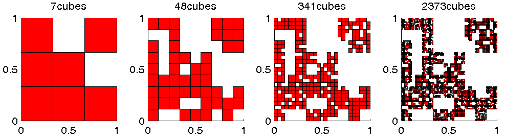
Refer to caption
Figure 5. Here, k=3,m=2k=3,m=2 and h=7h=7. We divide every cube into 9 smaller cubes and then pick about 7 ones from them with some randomness. For any particular cube, if the number of cubes picked at the current stage is less than (or respectively greater than) the desired one (i.e. 7), more (or respectively less) smaller cubes inside it will be picked for the next generation.

For any B∈ℬnB\in\mathcal{B}_{n}, suppose

λ2≤c​a​r​d​{B∗∈ℬn+j:B∗⊂B}hj≤λ1\lambda_{2}\leq\frac{card\left\{B^{\ast}\in\mathcal{B}_{n+j}:B^{\ast}\subset B\right\}}{h^{j}}\leq\lambda_{1}

whenever jj is large enough for some constants 0<λ2≤λ10<\lambda_{2}\leq\lambda_{1}. Define {𝐚n},\left\{\mathbf{a}_{n}\right\}, ℬ\mathcal{B} and μ\mu as before. Thus, when jj is large enough

Nn+j\displaystyle N_{n+j} =\displaystyle= ∑B∈ℬnc​a​r​d​{B∗∈ℬn+j:B∗⊂B}\displaystyle\sum_{B\in\mathcal{B}_{n}}card\left\{B^{\ast}\in\mathcal{B}_{n+j}:B^{\ast}\subset B\right\}
≤\displaystyle\leq ∑B∈ℬnλ1​hj=λ1​Nn​hj.\displaystyle\sum_{B\in\mathcal{B}_{n}}\lambda_{1}h^{j}=\lambda_{1}N_{n}h^{j}.

Then,

μ⁡(B)\displaystyle\mu\left(B\right) =\displaystyle= limj𝐚n+j​(B)\displaystyle\lim_{j}\mathbf{a}_{n+j}\left(B\right)
=\displaystyle= limjc​a​r​d​{B∗∈ℬn+j:B∗⊂B}Nn+j\displaystyle\lim_{j}\frac{card\left\{B^{\ast}\in\mathcal{B}_{n+j}:B^{\ast}\subset B\right\}}{N_{n+j}}
≥\displaystyle\geq limjλ2​hjλ1​Nn​hj=λNn​ for ​λ=λ2λ1​.\displaystyle\lim_{j}\frac{\lambda_{2}h^{j}}{\lambda_{1}N_{n}h^{j}}=\frac{\lambda}{N_{n}}\text{ for }\lambda=\frac{\lambda_{2}}{\lambda_{1}}\text{.}

Therefore, in this case, μ\mu is still evenly concentrated on a nested collection ℬ\mathcal{B}.

Recall that a nonnegative Borel measure μ\mu is Ahlfors regular of dimension dd if there exists a constant C>0C>0 such that

C−1​rd≤μ⁡(B⁡(x,r))≤C​rdC^{-1}r^{d}\leq\mu\left(B\left(x,r\right)\right)\leq Cr^{d}

whenever 0<r≤d​i​a​m​(s​p​t​(μ))0<r\leq diam\left(spt\left(\mu\right)\right) and xx lies in the support s​p​t​(μ)spt\left(\mu\right) of μ\mu.

Example 3.4.4.

If μ\mu is an Ahlfors regular measure whose support is a box B~\tilde{B} in ℝm\mathbb{R}^{m} , then μ\mu is evenly concentrated on a nested collection.

Proof.

By splitting the box B~\tilde{B} into smaller boxes of length size σn\sigma^{n}, we get a collection ℬn\mathcal{B}_{n} of disjoint boxes. For any B∈ℬnB\in\mathcal{B}_{n}, we have

a​(σn)d≤μ⁡(B)≤A​(σn)da\left(\sigma^{n}\right)^{d}\leq\mu\left(B\right)\leq A\left(\sigma^{n}\right)^{d}

for some dd and for some suitable constants a,A>0a,A>0. Thus,

μ⁡(B~)=∑B∈ℬnμ⁡(B)≤∑B∈ℬnA​(σn)d≤A​Nn​σn​d\mu\left(\tilde{B}\right)=\sum_{B\in\mathcal{B}_{n}}\mu\left(B\right)\leq\sum_{B\in\mathcal{B}_{n}}A\left(\sigma^{n}\right)^{d}\leq AN_{n}\sigma^{nd}

where NnN_{n} is the cardinality of the collection ℬn\mathcal{B}_{n}. Therefore, for every B∈ℬnB\in\mathcal{B}_{n}

μ⁡(B)≥a​σn​d≥a​μ⁡(B~)A​Nn=λNn\mu\left(B\right)\geq a\sigma^{nd}\geq a\frac{\mu\left(\tilde{B}\right)}{AN_{n}}=\frac{\lambda}{N_{n}}

where λ=aA​μ​(B~)>0\lambda=\frac{a}{A}\mu\left(\tilde{B}\right)>0. Hence, μ\mu is evenly concentrated on a nested collection. ∎

Definition 3.4.5.

For any Radon measure μ\mu, we define

dimU(μ):=inf{dimM(ℱ)}\dim_{U}\left(\mu\right):=\inf\left\{\dim_{M}\left(\mathcal{F}\right)\right\}

where the infimum is over all nested collection ℱ\mathcal{F} that μ\mu is evenly concentrated on.

Obviously,

dimM(μ)≤dimU(μ).\dim_{M}\left(\mu\right)\leq\dim_{U}\left(\mu\right).

Now, we have the following theorem for any α<1\alpha<1.

Theorem 3.4.6.

Suppose μ\mu is a probability measure with dimU(μ)<11−α\dim_{U}(\mu)<\frac{1}{1-\alpha} for some α<1\alpha<1, then μ∈𝒟α\mu\in\mathcal{D}_{\alpha}.

Proof.

Since dimM(μ)≤dimU(μ)\dim_{M}\left(\mu\right)\leq\dim_{U}\left(\mu\right), by theorem 3.3.5, μ∈𝒟α\mu\in\mathcal{D}_{\alpha} whenever 0≤α<10\leq\alpha<1. Thus, we only need to consider the case that α<0\alpha<0. Since dimU(μ)<11−α\dim_{U}(\mu)<\frac{1}{1-\alpha}, μ\mu is evenly concentrated on a nested collection ℱ\mathcal{F} with

dimM(ℱ)<11−α.\dim_{M}\left(\mathcal{F}\right)<\frac{1}{1-\alpha}.

For each cube QinQ_{i}^{n} in ℱ\mathcal{F}, if QinQ_{i}^{n} has no brothers, then l⁡(Qin)=0l\left(Q_{i}^{n}\right)=0. If QinQ_{i}^{n} has more than one brother, then

μ⁡(Qin)≥λNn​ and ​l​(Qin)≤C2​σn−1​.\mu\left(Q_{i}^{n}\right)\geq\frac{\lambda}{N_{n}}\text{ and }l\left(Q_{i}^{n}\right)\leq C_{2}\sigma^{n-1}\text{.}

Thus, when α≤0\alpha\leq 0, we always have

μ​(Qin)α​l​(Qin)≤(λNn)α​C2​σn−1.\mu\left(Q_{i}^{n}\right)^{\alpha}l\left(Q_{i}^{n}\right)\leq\left(\frac{\lambda}{N_{n}}\right)^{\alpha}C_{2}\sigma^{n-1}.

Therefore,

∑i=1Nnμ​(Qin)α​l​(Qin)≤C2​λασ​(Nn)1−α​σn.\sum_{i=1}^{N_{n}}\mu\left(Q_{i}^{n}\right)^{\alpha}l\left(Q_{i}^{n}\right)\leq\frac{C_{2}\lambda^{\alpha}}{\sigma}\left(N_{n}\right)^{1-\alpha}\sigma^{n}.

By lemma 3.3.3, we still have μ∈𝒟α\mu\in\mathcal{D}_{\alpha} when α≤0\alpha\leq 0. ∎

3.5. Comparison of dimensions of measures

Definition 3.5.1.

For any probability measure μ\mu, we define the transport dimension of μ\mu to be

dimT(μ)=infα<1{11−α:μ∈𝒟α​(ℝm)}.\dim_{T}\left(\mu\right)=\inf_{\alpha<1}\left\{\frac{1}{1-\alpha}:\mu\in\mathcal{D}_{\alpha}(\mathbb{R}^{m})\right\}.
Theorem 3.5.2.

Let μ\mu be any positive probability measure on ℝm\mathbb{R}^{m}. Then, the following bounds hold

dimH(μ)≤dimT(μ)≤m​a​x​{dimM(μ),1}.\dim_{H}(\mu)\leq\dim_{T}(\mu)\leq max\{\dim_{M}(\mu),1\}.

Moreover, we also have

dimH(μ)≤dimT(μ)≤dimU(μ).\dim_{H}(\mu)\leq\dim_{T}(\mu)\leq\dim_{U}(\mu).
Proof.

Assume that dimT(μ)>max⁡{dimM(μ),1}\dim_{T}(\mu)>\max\{\dim_{M}(\mu),1\} (or dimU(μ)\dim_{U}(\mu), respectively ). Then, we may pick an α<1\alpha<1 so that

dimT(μ)>11−α>max{dimM(μ),1} (or dimU(μ) respectively).\dim_{T}(\mu)>\frac{1}{1-\alpha}>\max\{\dim_{M}(\mu),1\}\text{ }\left(\text{or }\dim_{U}\left(\mu\right)\text{ respectively}\right).

By Theorem 3.3.5 (or Theorem 3.4.6), μ∈𝒟α​(ℝm)\mu\in\mathcal{D}_{\alpha}(\mathbb{R}^{m}). This is a contradiction to the definition of dimT(μ)\dim_{T}\left(\mu\right).

On the other hand, by Theorem 3.2.1, dimH(μ)≤11−α\dim_{H}(\mu)\leq\frac{1}{1-\alpha} whenever μ∈𝒟α​(ℝm)\mu\in\mathcal{D}_{\alpha}(\mathbb{R}^{m}). Thus, dimH(μ)≤dimT(μ)\dim_{H}(\mu)\leq\dim_{T}(\mu). ∎

Example 3.5.3.

Let μ\mu be the Cantor measure as in Example 3.1.3. Let QinQ_{i}^{n} denotes the it​hi^{th} Cantor interval of length 13n\frac{1}{{}^{3^{n}}}. Then, clearly μ\mu is evenly concentrated on the nested collection 𝒞={Qin:i=,2,⋯,2n}n=1∞\mathcal{C}=\left\{Q_{i}^{n}:i=,2,\cdots,2^{n}\right\}_{n=1}^{\infty}. Note that

dimM(𝒞)=limn→∞log⁡(Nn)log⁡(3n)=limn→∞log⁡(2n)log⁡(3n)=ln⁡2ln⁡3.\dim_{M}\left(\mathcal{C}\right)=\lim_{n\rightarrow\infty}\frac{\log\left(N_{n}\right)}{\log\left(3^{n}\right)}=\lim_{n\rightarrow\infty}\frac{\log\left(2^{n}\right)}{\log\left(3^{n}\right)}=\frac{\ln 2}{\ln 3}.

On the other hand, by lemma 3.2.4, dimH(μ)=ln⁡2ln⁡3\dim_{H}\left(\mu\right)=\frac{\ln 2}{\ln 3}. Therefore, by theorem 3.5.2,

dimT(μ)=ln⁡2ln⁡3.\dim_{T}\left(\mu\right)=\frac{\ln 2}{\ln 3}.

4. The Dimensional Distance between probability measures

For any α<1\alpha<1, let

𝒮α(ℝm)={Λ(μ−ν):Λ≥0,μ,ν∈𝒟α(ℝm)}\mathcal{S}_{\alpha}\left(\mathbb{R}^{m}\right)=\left\{\Lambda\left(\mu-\nu\right):\Lambda\geq 0,\mu,\nu\in\mathcal{D}_{\alpha}(\mathbb{R}^{m})\right\}

be a collection of signed measures. Clearly, 𝒮α1​(ℝm)⊆𝒮α2​(ℝm)\mathcal{S}_{\alpha_{1}}\left(\mathbb{R}^{m}\right)\subseteq\mathcal{S}_{\alpha_{2}}\left(\mathbb{R}^{m}\right) if α1≤α2\alpha_{1}\leq\alpha_{2}.

Definition 4.0.1.

For any two probability measures μ,ν\mu,\nu on ℝm\mathbb{R}^{m}, we define

D⁡(μ,ν):=infα<1{11−α:μ−ν∈𝒮α​(ℝm)}.D(\mu,\nu):=\inf_{\alpha<1}\{\frac{1}{1-\alpha}:\mu-\nu\in\mathcal{S}_{\alpha}\left(\mathbb{R}^{m}\right)\}.
Proposition 4.0.2.

D⁡(μ,ν)D\left(\mu,\nu\right)\, is a pseudometric11 1 A pseudometric DD means that it is nonnegative, symmetric, satisfies the triangle inequality, and D⁡(μ,μ)=0D\left(\mu,\mu\right)=0. But D⁡(μ,ν)=0D\left(\mu,\nu\right)=0 does not imply μ=ν\mu=\nu. on the space of probability measures on ℝm\mathbb{R}^{m}.

Proof.

It is clear that DD is symmetric and nonnegative. Also, for any α<1\alpha<1, μ−μ∈𝒮α\mu-\mu\in\mathcal{S}_{\alpha}, so D⁡(μ,μ)=0D(\mu,\mu)=0. Now we only need to check the triangle inequality:

(4.1) D⁡(μ1,μ2)+D⁡(μ2,μ3)≥D⁡(μ1,μ3),D(\mu_{1},\mu_{2})+D(\mu_{2},\mu_{3})\geq D(\mu_{1},\mu_{3}),

for any probability measures μ1,μ2,μ3\mu_{1},\mu_{2},\mu_{3} on ℝm\mathbb{R}^{m}.

Note that (4.1) is clearly true if either D⁡(μ1,μ2)D(\mu_{1},\mu_{2}) or D⁡(μ2,μ3)D(\mu_{2},\mu_{3}) is infinity. Thus we may assume that both D⁡(μ1,μ2)D(\mu_{1},\mu_{2}) and D⁡(μ2,μ3)D(\mu_{2},\mu_{3}) are finite. So, μ1−μ2∈𝒮α1\mu_{1}-\mu_{2}\in\mathcal{S}_{\alpha_{1}} and μ2−μ3∈𝒮α2\mu_{2}-\mu_{3}\in\mathcal{S}_{\alpha_{2}} for some α1,α2<1\alpha_{1},\alpha_{2}<1. Now,

μ1−μ3=(μ1−μ2)+(μ2−μ3)∈𝒮max⁡{α1,α2}​(ℝm).\mu_{1}-\mu_{3}=\left(\mu_{1}-\mu_{2}\right)+\left(\mu_{2}-\mu_{3}\right)\in\mathcal{S}_{\max\left\{\alpha_{1},\alpha_{2}\right\}}\left(\mathbb{R}^{m}\right).

Therefore,

D⁡(μ1,μ3)≤11−max⁡{α1,α2}≤11−α1+11−α2.D(\mu_{1},\mu_{3})\leq\frac{1}{1-\max\left\{\alpha_{1},\alpha_{2}\right\}}\leq\frac{1}{1-\alpha_{1}}+\frac{1}{1-\alpha_{2}}.

By taking an infimum over α1\alpha_{1} and α2\alpha_{2} we obtain the triangular inequality (4.1). ∎

In general, DD is not necessarily a metric. Indeed, for any two atomic probability measures 𝐚,𝐛\mathbf{a,b} , we have 𝐚−𝐛∈𝒮α​(ℝm)\mathbf{a-b\in}\mathcal{S}_{\alpha}\left(\mathbb{R}^{m}\right) for any α<1\alpha<1. Thus, D⁡(𝐚,𝐛)=0D\left(\mathbf{a,b}\right)=0 while 𝐚\mathbf{a} and 𝐛\mathbf{b} are not necessarily the same measure. Nevertheless, we may easily extend the pseudometric DD to a metric on equivalent classes of measures. To this end we define a notion of the equivalence classes on measures.

Definition 4.0.3.

For any two probability measures μ\mu and ν\nu on ℝm\mathbb{R}^{m}, we say

μ∼ν​ if ​D​(μ,ν)=0.\mu\sim\nu\text{\ if }D(\mu,\nu)=0.

The equivalent class of μ\mu is denoted by [μ][\mu].

For instance, all atomic probability measures are equivalent to each other.

Proposition 4.0.4.

If μ1∼μ2\mu_{1}\sim\mu_{2} and ν1∼ν2\nu_{1}\sim\nu_{2}, then D⁡(μ1,ν1)=D⁡(μ2,ν2).D(\mu_{1},\nu_{1})=D(\mu_{2},\nu_{2}).

Proof.

By definition of equivalence of measures we have D⁡(μ1,μ2)=0D(\mu_{1},\mu_{2})=0 and D⁡(ν1,ν2)=0D(\nu_{1},\nu_{2})=0. So by the triangular inequality (4.1) we have

|D⁡(μ1,ν1)−D⁡(μ2,ν2)|≤D⁡(μ1,μ2)+D⁡(ν1,ν2)=0.|D(\mu_{1},\nu_{1})-D(\mu_{2},\nu_{2})|\leq D(\mu_{1},\mu_{2})+D(\nu_{1},\nu_{2})=0.

∎

Definition 4.0.5.

For any equivalent class [μ][\mu] and [ν][\nu], define

𝐃⁡([μ],[ν])=D⁡(μ,ν).\mathbf{D}([\mu],[\nu])=D(\mu,\nu).

From this definition and proposition 4.0.2, clearly, we have the following theorem.

Theorem 4.0.6.

𝐃\mathbf{D} is a metric on 𝒫(ℝm)/∼\mathcal{P}\left(\mathbb{R}^{m}\right)/\sim .

Definition 4.0.7.

The metric 𝐃\mathbf{D} is called the dimensional distance on the space 𝒫(ℝm)/∼\mathcal{P}\left(\mathbb{R}^{m}\right)/\sim of equivalent classes of probability measures on ℝm\mathbb{R}^{m}.

We now give a geometric meaning to transport dimension of measures.

Theorem 4.0.8.

For any positive probability measure μ\mu, we have

dimT(μ)=𝐃⁡([μ],[𝐚])=D⁡(μ,𝐚)\dim_{T}(\mu)=\mathbf{D}\left(\left[\mu\right],\left[\mathbf{a}\right]\right)=D(\mu,\mathbf{a})

where 𝐚\mathbf{a} is any atomic probability measure.

Proof.

Since 𝐚∈𝒟α\mathbf{a\in}\mathcal{D}_{\alpha} for any α<1\alpha<1, we have

D⁡(μ,𝐚)\displaystyle D(\mu,\mathbf{a}) =\displaystyle= infα<1{11−α:μ−𝐚∈Sα}\displaystyle\inf_{\alpha<1}\{\frac{1}{1-\alpha}:\mu-\mathbf{a}\in S_{\alpha}\}
=\displaystyle= infα<1{11−α:μ∈𝒟α}=dimT(μ).\displaystyle\inf_{\alpha<1}\{\frac{1}{1-\alpha}:\mu\in\mathcal{D}_{\alpha}\}=\dim_{T}\left(\mu\right).

∎

This theorem says that the transport dimension of a probability measure μ\mu is the distance from μ\mu to any atomic measure with respect to the dimensional distance. In other words, the dimension information of a measure tells us quantitatively how far the measure is from being an atomic measure.

References

  • [1] A. Brancolini, G. Buttazzo, F. Santambrogio, Path functions over Wasserstein spaces. J. Eur. Math. Soc. Vol. 8, No.3 (2006),415–434.
  • [2] M. Bernot; V. Caselles; J. Morel, Traffic plans. Publ. Mat. 49 (2005), no. 2, 417–451.
  • [3] M. Bernot; V. Caselles; J. Morel; Optimal Transportation Networks: Models and Theory. Series: Lecture Notes in Mathematics , Vol. 1955 , (2009).
  • [4] Thierry De Pauw and Robert Hardt. Size minimization and approximating problems, Calc. Var. Partial Differential Equations 17 (2003), 405-442.
  • [5] L.C. Evans and R. Gariepy. Measure theory and fine properites of functions. Stud. Adv. Math., CRC Press, 1992
  • [6] E.N. Gilbert, Minimum cost communication networks, Bell System Tech. J. 46, (1967), pp. 2209-2227.
  • [7] F. Maddalena, S. Solimini and J.M. Morel. A variational model of irrigation patterns, Interfaces and Free Boundaries, Volume 5, Issue 4, (2003), pp. 391-416.
  • [8] G. Devillanova and S. Solimini. On the dimension of an irrigable measure. Rend. Semin. Mat. Univ. Padova 117 (2007), 1–49.
  • [9] E. Paolini and E. Stepanov. Optimal transportation networks as flat chains. Interfaces and Free Boundaries, 8 (2006), 393-436.
  • [10] B. White. Rectifiability of flat chains. Annals of Mathematics 150 (1999), no. 1, 165-184.
  • [11] Q. Xia, Optimal paths related to transport problems. Communications in Contemporary Mathematics. Vol. 5, No. 2 (2003) 251-279.
  • [12] Q. Xia. Interior regularity of optimal transport paths. Calculus of Variations and Partial Differential Equations. 20 (2004), no. 3, 283–299.
  • [13] Q. Xia, An application of optimal transport paths to urban trasnport networks. Discrete and Continuous Dynmical Systems, Supp. 2005, pp 904-910.
  • [14] Q. Xia. Boundary regularity of optimal transport paths. Preprint.
  • [15] Q. Xia. The formation of tree leaf. ESAIM Control Optim. Calc. Var. 13 (2007), no. 2, 359–377.
  • [16] Q. Xia. The geodesic problem in quasimetric spaces. Journal of Geometric Analysis: Volume 19, Issue2 (2009), 452–479.
  • [17] Q. Xia and D. Unger, Diffusion-limited aggregation driven by optimal transportation. Preprint.
  • [18] G. Xue, T. Lillys and D. Dougherty. Computing the Minimum Cost Pipe Network Interconnecting One Sink and Many Sources. SIAM Journal on Optimization. Volume 10 , Issue 1 (1999) Pages: 22 - 42 .
  • [19] Zhang and Zhu. A bilevel programming method for pipe network optimization. SIAM Journal on Optimization, Vol 6, 838 (1996).