A self-contained guide to the CMB Gibbs sampler
Abstract
We present a consistent self-contained and pedagogical review of the CMB Gibbs sampler, focusing on computational methods and code design. We provide an easy-to-use CMB Gibbs sampler named SLAVE developed in C++ using object-oriented design. While discussing why the need for a Gibbs sampler is evident and what the Gibbs sampler can be used for in a cosmological context, we review in detail the analytical expressions for the conditional probability densities and discuss the problems of galactic foreground removal and anisotropic noise. Having demonstrated that SLAVE is a working, usable CMB Gibbs sampler, we present the algorithm for white noise level estimation. We then give a short guide on operating SLAVE before introducing the post-processing utilities for obtaining the best-fit power spectrum using the Blackwell-Rao estimator.
Subject headings
cosmic microwave background — cosmology: observations — methods: numericalI. Introduction
In recent years, increased resolution in the measurement of the cosmic microwave background (CMB) have driven the need for more accurate data analysis techniques. During the early years of CMB experiments, data was so sparse and noise levels so high that error bars in general overshadowed the observed signal. With the COBE experiment, [24] posteriors were mapped out by brute force, and the statistical methods employed were simplistic. This was sufficient, as advanced statistical methods weren’t needed for analyzing crude data. However, all this changed with the Wilkinson Microwave Anisotropy Probe (WMAP) experiment [1, 16]. Suddenly, cosmological data became much more detailed, vastly improving our knowledge of the universe, but also introduced new problems. Which parts of the signal were pure CMB, and which were not? The need for knowledge about instrumental noise, point sources, dust emission, synchrotron radiation and other contaminations were required in order to estimate the pure CMB signal from the data. And, how does one properly deal with the the sky cut, the contamination from our galaxy? Even harder, how does one maximize the probability that the resulting signal really is the correct CMB signal? A new era of cosmological statistics emerged.
An important event was the introduction of Bayesian statistics in cosmological data analysis. Bayesian statistics differs from the frequentist thought by quantizing ignorance: what one knows and not knows are intrinsic parts of the analysis. The goal of any Bayesian analysis is to go from the prior , or what is known about the model, to the posterior , the probability of a model given data. This is summarized via Bayes’ famous theorem:
| (1) |
The posterior tells us something about how well a model fits the data, and is obtained by multiplying the prior , our assumption of the model, with the likelihood , the probability that the data fits the model.
The need for Bayesian statistics becomes evident when considering that we only have data from one single experiment to analyze. Bayesian statistics merges with frequentist statistics for large number of samples. And, in a cosmological context, we are stuck with only one sample, a sample that we are constantly measuring to higher accuracies. This sample is one realization of the underlying universe model, and we are unable to obtain data from another sample.
In a standard Metropolis-Hastings (MH) Monte Carlo Markov chain-approach (MCMC), one samples from the joint distribution by letting chains of “random walkers” transverse the parameter space. The posterior is obtained by calculating the normalized histogram of all the samples in the chains. The posterior will eventually resemble the underlying joint distribution, or the likelihood surface. This is a simple and easy-to-understand approach, but not without drawbacks. For one, each MH step is required to test the likelihood value of the chain at the current position in parameter space up against a new proposed position. Many of these steps will be rejected, and this is where the computational costs usually reside. The Gibbs sampler provides something new: one never needs to reject samples, and every move becomes accepted and usable for building the posterior. This is done by assuming that we have prior knowledge of the conditional distributions. These are then sampled from, each in turn yielding accepted steps.
However, the main motivation for introducing the CMB Gibbs sampler is the drastically improvement in scaling. With conventional MCMC methods, one needs to sample from the joint distribution, which results in an operation. For a white noise case, the Gibbs sampler splits the sampling process into independently sampling from the two conditional distributions, which together yields a operation. In other words, the Gibbs sampler enables sampling the high- regime much more effective than previous MCMC methods.
The problem of estimating the cosmological signal from the full signal by Gibbs sampling was first addressed in Jewell et al. [19], Wandelt et al. [25] and Eriksen et al. [9]. The ultimate goal of the Gibbs sampler is to estimate the CMB signal from the data , eliminating noise , convolution , all while including the sky cut. Today, a great number of papers have employed the Gibbs sampler since the introduction of the method [11, 12, 7, 4, 14, 15, 10, 20, 18, 5, 3, 6, 21].
In this paper, we review the basics of the CMB Gibbs sampler, and provide a simple, intuitive non-parallelized CMB Gibbs software bundle named SLAVE. SLAVE is written in C++, and employs object-oriented design in order to simplify mathematical implementation. The OOP design of SLAVE is presented in figure 1. For instance, assuming and are instances of the “real alm” class (they contain a set of real s), operator overloading enables us to directly translate the expression by writing
A = (B+C).Invert();
This yields fast code that closely resembles equations, without having optimized too much for parallel computing, multiple data sets and other complexities.

I.1. The Master algorithm
One method of likelihood-estimator for obtaining the best-fit power spectrum for masked CMB data is given by the MASTER algorithm [17]. While Gibbs sampling estimates the full CMB signal , the MASTER method only estimates the power spectrum. This method does not allow for variations in the estimated signal, except for the natural variations from simulating different realizations from the same power spectrum. However, the master algorithm estimates the power spectrum with cost scaling as , which is slow for high- operations.
I.2. What do I need the CMB Gibbs sampler for?
Often, people misunderstand the concepts behind the CMB Gibbs sampler, and what the Gibbs sampler can be used for. In this section, we try to explain in simple terms when you should consider employing the CMB Gibbs sampler.
Assume that you have a theoretical universe model , where is a set of cosmological parameters. This model might give rise to some additional gaussian effects in the CMB map, either as fluctuations, altered power, anisotropic contributions, dipoles, ring structures or whatever. You now wish to test whether existing CMB data contains traces of your fabulous new model, and how significant those traces are. Or maybe you are just interested in ruling out the possibility that this model could be observed at all.
In any case, you need to implement some sort of numerical library that generates CMB maps based on your model. These maps will be “pure”, in the sense that you have complete control over its generation process and systematics. Assume that your model has 1 free parameter. You could now loop over the 1-dimensional parameter space and calculate the between a pure CMB signal map and the map from your model. This would have to be done for each step in parameter space, before obtaining the minimum. Even better, you could implement a Monte Carlo Markov chain framework, letting random walkers traverse a likelihood surface, yielding posteriors. This would enable support for a larger number of parameters, and is superior to the slow brute force approach.
In real-life however, things are not this simple. Data from any CMB experiment is contaminated by noise and foregrounds, most notably our own galaxy. This means that estimating the signal from the data is not trivial - one needs to “rebuild”, or make an assumption of what the fluctuations are within the sky cut and noise limits. This implies that it really isn’t possible to obtain “the correct” CMB map, all we can know is that there exist a statistical range of validity where a simulated map agrees with the true CMB signal. Therefore, the consideration that that the estimated CMB signal is a statistical random variable and not a fixed map should be included in the analysis. Hence, if you have implemented the MASTER method mentioned in section I.1, you should test your model map against a set of realizations from the MASTER-estimated signal power spectrum.
This is where the Gibbs sampler enters the stage. As previously mentioned, the Gibbs sampler will estimate the CMB signal given data, and not only the power spectrum. The Gibbs sampler also ensures that every step in parameter space is always valid, so one never needs to discard samples. And even better, each of these independent steps provide an operation cost for obtaining samples that are much lower than more conventional MCMC methods. In order to test whether your model fits the data, you therefore include the uncertainty in data by varying the signal. For example:
initialize Cl
do
  s = the CMB signal given the
       power spectrum Cl
  m = the CMB signal of your model given
       the estimated CMB signal s
  Cl = the CMB power spectrum given m
  save s, m and Cl
repeat until convergence
In the end, you calculate the statistical properties of s, m and Cl. Your model parameters have now been estimated, and the process included the intrinsic uncertainties in the signal. This method is not the most rapid - but it will always yield correct results.
II. The CMB Gibbs sampler
Throughout this paper, we assume that the data can be expressed as
| (2) |
where is the CMB signal, the instrument beam and uncorrelated noise.
The MASTER algorithm estimates the the power spectrum and the standard deviation . However, this method is a approximation to a full likelihood that can be expressed as follows:
| (3) |
where and are the signal and noise covariance matrices, respectively. While it is fully possible to use MCMC-methods to sample from this distribution, the calculation of the -matrix scales as , where is the size of the matrix. This is therefore an extremely slow operation, and is not feasible for large s. If we demand that we sample the sky signal as well, the joint distribution becomes . This might seem unnecessary complicated, as one most of the time doesn’t need the signal . But when feeding this distribution through the Gibbs sampler - that is, calculating the conditional distributions and , we find that sampling from both are computationally faster than sampling from the full distribution in equation 3. The derivations of the conditional distributions are presented in section III.
II.1. Review of the Metropolis-Hastings algorithm
The Gibbs sampler is a special case of the Metropolis-Hastings algorithm. We therefore review the basics of Monte Carlo Markov (MCMC) chain methods. The Metropolis-Hastings algorithm is a MCMC method for sampling directly from a probability distribution. This is done by letting “random walkers” transverse a parameter space, guided by the likelihood function, the probability that the data fits the model for the given parameter configuration. If a proposal step yields a likelihood greater than the current likelihood, then random walker accepts the step immediately. If the likelihood is less, then the walker will with a certain probability step “down” the likelihood surface. Eventually, the histogram of all the random walkers will converge to the posterior, the full underlying distribution.
Assume you have a model with parameters, and you wish to map out a joint distribution from . Usually, one calculates the ratio between the posteriors at the two steps and , such that
| (4) |
where is the proposal distribution for going left or right. If the proposal distribution is symmetric (i.e. the probability of going left-right is equal for all ), then such that:
| (5) |
The MH acceptance rule now states: if is larger than 1, accepted the step unconditionally. If , then accept the step if a random uniform variable .
II.2. Review of the Gibbs algorithm
Assume you have a model with two parameters, and , and you wish to map out a joint distribution from . Now, also presume that you have prior knowledge of the conditional distributions, and . A general proposal density is not necessary symmetric, and one must therefore consider the asymmetric proposal term as described in equation 4. However, we now define the proposal density for to be the conditional distributions:
| (6) |
In words, the proposal is only considered when , which means that is fixed while can vary. If so, the acceptance is then given as the conditional distribution , which we must have prior knowledge of. The reason for choosing such a proposal density becomes clear when investigating the Metropolis Hastings acceptance rate:
| (7) |
Using the conditional sampling proposal (6) one obtains
| (8) |
We now enforce the delta-function such that . This sampling from the conditional distributions is the crucial step in the Gibbs sampler, such that all terms cancel out:
| (9) |
This implies that all steps are valid, and none are ever rejected. Hence one alternates between sampling from the known conditional distributions, where each step is independently accepted and can be performed as many times as needed.
III. The conditional distributions
In section II.2, it was explained how the Gibbs sampler requires previous knowledge about the underlying conditional distributions. The CMB Gibbs sampler will alternate between sampling power spectra and CMB signal , where each proposed step will always be valid. In order to enable sampling from the joint distribution, we therefore need to derive the analytical properties of the conditional distributions:
| (10) |
The derivations described here were first presented in Jewell et al. [19], Wandelt et al. [25] and Eriksen et al. [9].The full, joint distribution is expressed as
| (11) | |||||
| (12) |
where is a prior on , typically chosen to be flat. The first term, , is nothing but the . The measures the goodness-of-fit between model and data, leaving only fluctuations in noise. As is distributed accordingly to a Gaussian with mean 0 and variance , we find that
| (13) |
As we now assume that the signal is known and fixed, the data becomes redundant and . We therefore first need to obtain an expression for .
III.1. Deriving
Assuming that the CMB map consists of Gaussian fluctuations, we can express the conditional probability density for a power spectrum given a sky signal as follows:
| (14) |
where is the covariance matrix. We now perform a transformation to spherical harmonics space, where and . Then equation (14) transforms to
| (15) |
As the spherical harmonics are orthogonal, they all cancel out and leave delta functions for such that
| (16) |
We now define a power spectrum such that
| (17) |
Similarly, the determinant is given as the product of the diagonal matrix , which for each has values of . The determinant is thus . Expression (14) can now be written as
| (18) |
which by definition means that the ’s are distributed as an inverse Gamma function. In the computational section, we will discuss how to draw random variables from this distribution.
III.2. Deriving
Again, we begin with the full, joint distribution:
| (19) |
We now know from equation 18 and 13 that the joint distribution can be expressed as
| (20) |
omitting the prior . Again, note that it would be nearly impossible to sample directly from the full distribution. We now investigate what happens with equation 20 when becomes a fixed quantity. As the s in the denominator vanishes, we use equation 14 to obtain
| (21) |
We now introduce a residual variable , such that roughly consist of noise. As noise was uncorrelated, we can expect that follows a Gaussian distribution with zero mean and variance. Also, if is known, then is redundant. We complete the square, and introduce . Equation (21) can now be rewritten as
| (22) |
Hence is a Gaussian distribution with mean and covariance . In the computational section, we will discuss how to draw random variables from this distribution.
IV. Numerical implementation
In its utter simplicity, the mechanics of the Gibbs sampler can be summarized as follows:
 load data
 initialize s and cl
 loop number of chains
   s = generate from p(s | cl, d)
   cl = generate from p(cl | s, d)
   save s and cl
 end loop
We now present the computational methods for drawing from and .
IV.1.
We show that equation 18 is an inverse Gamma distribution. A general gamma-distribution is proportional to
| (23) |
Equation 18 can be expressed as
| (24) |
where . If we now perform a substitution , we see that
| (25) |
where the last term is the Jacobian. Hence
| (26) |
which is a gamma-distribution for . We now show that this particular distribution also happens to be a special case of the distribution:
| (27) |
Letting and ignoring the constants, we find that
| (28) |
such that if , is distributed according to a distribution with degrees of freedom. A random variable following such a distribution can be drawn as follows:
| (29) |
where are random Gaussian variables with mean and variance . Since , we find that
| (30) |
Numerically, one can implement this as
 for each l
  z = 0
  for i=0 to 2l-1
    z = z+ rand_gauss()^2
  end
  C(l) = (2l+1)*sigma(l)/z
end
An example of this method can be found in the SLAVE libraries, within class “powerspectrum” method “draw_gamma”.
IV.2.
From equation 22, it is easy to see that is a Gaussian distribution with mean and variance . Instead of deriving a method for drawing a random variable from this distribution, we present the solution and show that this solution indeed has the necessary properties [19]. Let
| (31) |
where and are independent, random variables. We now show that the random variable indeed has mean and variance . First,
| (32) |
As ,
| (33) |
by definition.
The covariance is then
| (34) |
Note that in the term , we have , so we are only left with the terms with the random variables :
But, as and are independently drawn from a distribution, then , and we end up with
| (35) |
which shows that a random variable drawn using equation 31 has the desired properties of being drawn from .
Having implemented a “real alm” class in SLAVE with operator overloading, it is possible to directly translate equation 31 into code:
  omega1.gaussian_draw(0, 1, rng);
  omega2.gaussian_draw(0, 1, rng);
  calculate_CNI();
  S = CNI* (NI*D + NI.square_root()*omega1
     + CI.square_root()*omega2);
where the code has been slightly optimized: both , and has been pre-calculated for efficiency. Note that this is only possible to do when assuming full-sky coverage with constant RMS noise. If the noise isn’t constant on the sky, then is a dense off-diagonal matrix, nearly impossible to calculate directly for large . However, it is still possible to perform the calculation in pixel space, but this requires that we assume to be an operator instead of a matrix. We will address this issue in section IV.6.
We have now presented the main simplified Gibbs-steps for calculating and , without convolution, uniform noise and no sky cut. Sampling from these two distributions is then done alternating between the two Gibbs steps, and the chain output - and - are saved to disk during each step.
We now investigate the behavior of these fields, as each have special properties.
IV.3. Field properties

Equation 31 can be broken into two separate parts: the Wiener filter and the fluctuation map . In figure 3, each of these maps are depicted. The Wiener filter map determines the fluctuations outside the sky cut - where they are heavily constrained by the known data, given cosmic variance and noise. However, within the sky cut, large-scale fluctuations are possible to pin down statistically while small-scales are repressed. The fluctuation map determines the small-scale fluctuations within the unknown sky cut, and are constrained by cosmic variance and noise effects. Outside the sky cut, the fluctuation map is constrained by the data, yielding very low small-scale fluctuations. The sum of these two parts make up the full CMB signal sample.
IV.4. Verifying the sample signal: the test
When the signal is being sampled, it is vital to check that the input parameters/data maps are correctly set up. For instance, if you use SLAVE to start a large job, say, estimating the CMB signal for a map, it can be very frustrating when realizing that one of the input parameters were incorrect, for instance beam convolution or noise RMS. The software will continue to run without errors, but the resulting output files will be incorrect. We therefore adopt a simple and useful method for verifying that the estimated CMB signal for each Gibbs step really is close to what one would expect.
The trick lies with the noise. As , then . Uniform white noise is assumed to be -distributed, so
| (36) |
A distribution is nothing but a sum of squared Gaussian distributions. Hence
| (37) |
and the should be close to the number of pixels in the map plus minus . Usually, when an incorrect parameter is used, the comes out far away from the expected value.
Calculating the is not particularly time-consuming, but it has other uses as well: the is used in the estimation of noise, as presented in section V.
IV.5. Convolution
A thing we did not address in the previous section was the inclusion of the instrumental beam convolution . Including this in equation 31, we obtain
| (38) |
In SLAVE, the beam is loaded directly from a fits file, or generated as a Gaussian beam given a full width half-maximum (FWHM) range. The beam is then multiplied with the corresponding pixel window, and stored in the -object throughout the code.
IV.6. The sky cut
Until now, we have only assumed full-sky data sets contaminated by constant noise. However, in order to be able to investigate real data, we need to take into account both the foreground galaxy and anisotropic noise. The galaxy contributes to almost 20% of the WMAP data, and needs to be removed with a mask. This means that the usable pars of the maps becomes anisotropic, giving rise to correlations in the spherical harmonics s. In other words, all the previously diagonal and well-behaved matrices now have off-diagonal elements, which for large is an impossible feat to perform for dense matrices.
One way to get around these problems is to perform the calculations containing the sky cut mask in pixel space. This means that every time one needs to take into account the sky cut, one transforms from harmonic to pixel space, performs the operation including the sky cut before transforming back to harmonic space. While this operation in itself is trivial, equation 31 provides a few other problems:
| (39) |
The right-hand side can easily be calculated, letting be an operator acting on and , switching from spherical harmonics to pixel space and back. However, the left-hand side is troublesome - one cannot solve this equation explicitly. First, we need to rewrite 39 a bit:
| (40) | |||
| (41) |
The first thing one should note about equation 41 is that the left-hand term is proportional to , where the diagonal parts are just the signal-to-noise ratios of the corresponding mode. Another nice feature about this form is that the variance of the signal is kept constant, that is, , but . Hence we obtain better numerical stability. In order to solve the equation , we implement a direct-from-textbook Conjugate Gradient (CG) algorithm presented on page 40 in [22]. The code looks like this:
  b = L*( A*NI(D) + A*NI(map_work2,true)) + omega2;
  MI = setup_preconditioner();
  x = mult_by_A(x);
  r =  b - x;
  d = MI*r;
  r0 = r.norm_L1(r);
  do {
    Ad = mult_by_A(d);
    alpha = r.dot(MI*r) / (d.dot(Ad));
    x = x + d*alpha;
    rn = r - Ad*alpha;
    beta = rn.dot(MI*rn) / (r.dot(MI*r));
    d = MI * rn + d*beta;
    r = rn;
    norm = r.norm_L1(r);
  }
  while (norm>r0*epsilon);
  S = L*x;
C++ enables the CG algorithm to be translated almost directly from mathematical syntax to code. Here, the sky cut mask is taken into account in the -method - one only needs the mask when multiplying with the inverse noise matrix. The only other “initial condition” is the preconditioner. The preconditioner cannot affect the result, that is, it has nothing to do with the estimated signal . The preconditioner only affects the number of iterations needed for the equation to be solved, and corresponds to a “best guess” of . Without going into details, the standard preconditioner in SLAVE is proportional to , but there exists many other suggestions for better pre-conditioners, yielding quicker convergence. See [8] or [23] for more examples.
When the CG search has completed, the signal has been obtained, including the sky cut and anisotropic noise.
IV.7. Low signal-to-noise regime
A final thing we need to take into account is the low signal-to-noise regime. When the noise starts dominating the signal, the estimated will fluctuate wildly on small scales. In addition, the deconvolution will add to this effect, blowing up noise to extreme values. In itself, this isn’t a bad thing as we really cannot say exactly what is going in this regime, but it will affect the overall correlations between chains. In order to reduce this effect, we present a simple way to bin multipoles together on large l, reducing noise variance.
Let be the noise RMS in harmonic space. The variance is then given as
| (42) |
For a single binned set with multipoles ranging from to , the average value of the power spectrum is given as
| (43) |
Similarly for the noise power spectrum,
| (44) |
Thus, the variance of the noise is given as
| (45) |
Obviously, is reduced as the number of multipoles in the bin is increased. We now select bins such that the noise variance in a single bin is always less than three times the value of the angular power spectrum, or .

The only affected part of the code is where one determines . Instead of generating a power spectrum given a set of , the calculation is now performed via a binning class that calculates the binned power spectrum . That is,
| (46) |
Absorbing the product into the exponential, this becomes
| (47) |
We now sample the signal with flat bins in , not in .
V. Generalizing the model: Noise estimation
In this section, we give a direct example of how one could extend the data model to the SLAVE Gibbs sampler. We derive the necessary conditional distribution, explain how this was integrated, and present some results from [15], where a full analysis of the noise levels in the WMAP data was performed using the SLAVE framework.
Traditionally, the noise properties used in the Gibbs sampler [8, e.g.,] have been assumed known to infinite precision. In this section, however, we relax this assumption, and introduce a new free parameter, , that scales the fiducial noise covariance matrix, , such that . Thus, if there is no deviation between the assumed and real noise levels, then should equal 1. The full analysis of the 5-yr WMAP data was presented in [15], with interesting results. For the foreground-reduced 5-year WMAP sky maps, we find that the posterior means typically range between and depending on differencing assembly, indicating that the noise level of these maps are underestimated by 0.5-1.0%. The same problem is not observed for the uncorrected WMAP sky maps.
The full joint posterior, , now includes the amplitude . We can rewrite this as follows:
| (48) |
where the first term is the likelihood,
| (49) |
the second term is a CMB prior, and the third term is a prior on . Note that the latter two are independent, given that these describe two a-priori independent objects. In this paper, we adopt a Gaussian prior centered on unity on , . Typically, we choose a very loose prior, such that the posterior is completely data-driven.
The conditional distribution for can now be expressed as
| (50) |
where and is the . (Note that the is already calculated within the Gibbs sampler, as it is used to validate that the input noise maps and beams are within a correct range for each Gibbs iteration. Sampling from this distribution within the Gibbs sampler represent therefore a completely negligible extra computational cost.) For the Gaussian prior with unity mean and standard deviation , we find that
| (51) |
For large degrees of freedom, , the inverse gamma function converges to a Gaussian distribution with mean , where we have defined , and variance . A good approximation is therefore letting be drawn from a product of two Gaussian distributions, which itself is a Gaussian, with mean and standard deviation
| (52) |
| (53) |
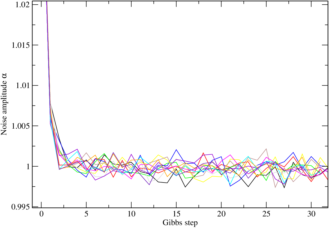
This sampling step has been implemented in SLAVE and we have successfully tested it on simulated maps. With and and full sky coverage, we find . The chains for the noise amplitude are shown in figure 5. Note that with such high resolution, the standard deviation on is extremely low, and any deviation from the exact will be detected.
VI. Running SLAVE
In this section, we quickly review how to use SLAVE. For a more detailed usage, please see the SLAVE documentation (when the framework will be released).
SLAVE requires the HEALPIX [13] CXX-libraries installed. Please see the HEALPIX documentation on this topic. SLAVE is run command-line, and requires a parameter file as command-line parameter. The most important options in the parameter file are listed in table 1.
| General parameters | ||
| seed | int | Initial random seed |
| verbosity | int | Text output level (0=none) |
| healpix_dir | string | HEALPIX home directory |
| output_sigmas | bool | Output or not |
| output_cls | bool | Output s or not |
| output_directory | string | Output file directory |
| output_chisq | bool | Output the or not |
| output_beam | bool | Output the beam or not |
| output_beam_file | string | Beam output filename |
| Operations | ||
| method | string | Analysis type: brute force_fullsky or CG (normal) |
| CG_convergence | double | CG Convergence criteria (type ) |
| preconditioner | string | Pre-conditioner type: none, static or 3j |
| init_powerspectrum_power | double | Initialized flat power spectrum value |
| init_powerspectrum_use_file | bool | Use file instead of flat power spectrum |
| init_powerspectrum_file | string | Initial power spectrum file |
| samples | int | Number of Gibbs samples to produce |
| burnin | int | Number of burn-in samples to reject |
| Data | ||
| datasets | int | Number of data sets (only 1 allowed yet..) |
| data_nsideN | int | for data set |
| data_mapN | string | FITS map for data set |
| data_rmsN | string | FITS rms map for data set |
| data_maskN | string | FITS mask for data set |
| beam_fileN | string | FITS beam for data set |
| lmax | int | for the analysis |
| constant_rms | bool | Use constant rms or not |
| constant_rms_value | double | Value of constant rms |
| gaussian_beam | bool | Use a Gaussian beam or not |
| gaussian_beam_fwhm | double | Value of Gaussian beam |
| Noise estimation parameters | ||
| enable_noise_amplitude_sampling | bool | Enable noise estimation or not |
| noise_sampling_sigma | double | The noise prior sigma |
| noise_amplitude_filename | string | Output noise filename |
| noise_alpha_init_val | double | Initial value for |
| Binning | ||
| use_binning | bool | Enable binning of power spectrum |
| binning_powerspectrum | string | Power spectrum used for binning |
| bins_filename | string | Text output the bins |
Note. — The SLAVE parameter names and usage may have changed when the first version is released.
VI.1. Post-processing
After the Gibbs sampler has been cooking for a while, it is time to investigate the results. The main output of SLAVE are the estimated power spectra ’s and the signals . However, as the signal is assumed to be statistically isotropic, we instead output the signal power spectra defined as:
| (54) |
The text-files may be plotted directly through software such as XMGRACE, as presented in figure 6.

In addition, SLAVE outputs the ’s as a binary file for each chain. These binary files can be combined through the main post-processing software utility for SLAVE called SLAVE_PROCESS. This software will combine the binary chains into a single file, in addition to removing burn-in samples. To combine the sigmas into one file, type
 slave_process 1 [no_chains] [no_samples]
                 [burnin] [output sigma_l file]

VI.2. likelihoods
The first important step is to verify that the output s follow the desired inverse-Gamma distribution for low , but converges to Gaussians for larger . The SLAVE processing utility SLAVE_PROCESS can generate a set of s from the s and output the corresponding values for a single . It is then straight-forward to use a graphical utility such as XMGRACE to obtain the histogram. Such histograms are plotted together with the analytical likelihoods in figure 7. Note the good match between the histogram of the s and the likelihoods obtained from the Blackwell-Rao estimator. The analysis for producing these plots was performed on simulated high-detail data, in order to verify the validity of the BR-estimator.
To save the cls for a specific , type
 ./process 4 [sigma_l file] [l] [generate no cls]
             [output textfile]
VI.3. The Blackwell-Rao estimator
Our primary objective is obtaining the best-fit power spectrum from the estimated signal power spectra. If the s were completely distributed according to a Gaussian, one would only need to select the maximum of the distribution for each . However, as we saw in equation 18, this is not the case, and we need a better way to obtain the likelihood for each .
Luckily, we can obtain an analytical expression of the likelihood for the s via the Blackwell-Rao (BR) estimator, as presented in [2]. By using prior knowledge of the distributions of the s, we can build an analytical expression for the distribution for each given the signal power spectrum , or .
Note that since the power spectrum only depends on the data through the signal and thus , then
| (55) |
It is therefore possible to approximate the distribution as such:
| (56) | |||||
| (57) | |||||
| (58) | |||||
| (59) |
where is the number of Gibbs samples in the chain. This method of estimating the is called the Blackwell-Rao estimator. Now, for a Gaussian field,
| (60) |
Taking the logarithm, we obtain a nice expression
| (61) |
which is straight-forward to implement numerically. To output the BR-estimated likelihood for one , type
 ./process 3 [sigma_l file] [l]
             [output likelihood]
VI.4. Power spectrum estimation
The best-fit BR-estimated power spectrum is obtained by choosing the maximum likelihood value of for each . To do so, type
 ./process 2 [sigma_l file]
             [output power spectrum file]
An example of a BR-estimated power spectrum can be seen in figure 8. In addition, both the input-and noise power spectra are shown. Note how the BR-estimated power spectrum is exact on small scales (low ), while the convolution and noise dominated on higher scales.

VII. Conclusions
We have presented a self-contained guide to a CMB Gibbs sampler, having focused on both deriving the conditional probability distributions and code design. We described in detail how one can draw samples from the conditional distributions, and saw how the Gibbs sampler is numerically superior to conventional MCMC methods, scaling as . We have also introduced a new object-oriented CMB Gibbs framework, which employs the existing HEALPix [13] C++ package. We presented a small guide to the usage of SLAVE, including post-processing tools and the Blackwell-Rao estimator for obtaining the likelihoods and the best-fit power spectrum. We also reviewed a new way of estimating noise levels in CMB maps, as presented in [15]. The software package SLAVE will hopefully be released when it is completed during 2009, and will run on all operating systems supporting the GNU C++ compiler. Please see http://www.irio.co.uk for release details and information.
References
- [1] Bennett, C. L., et al. 2003, ApJS, 148, 1
- [2] Chu, M., Eriksen, H. K., Knox, L., Górski, K. M., Jewell, J. B., Larson, D. L., O’Dwyer, I. J., & Wandelt, B. D. 2005, Phys. Rev. D, 71, 103002
- [3] Chu, I.-W. M. 2005, Ph.D. Thesis,
- [4] Cumberbatch, D. T., Zuntz, J., Kamfjord Eriksen, H. K., & Silk, J. 2009, arXiv:0902.0039
- [5] Dickinson, C., Eriksen, H. K., Jewell, J., Banday, A. J., Gorski, K. M., & Lawrence, C. R. 2007, Bulletin of the American Astronomical Society, 38, 883
- [6] Dickinson, C., et al. 2009, arXiv:0903.4311
- [7] Dunkley, J., et al. 2008, arXiv:0811.4280
- [8] Eriksen, H. K., et al. 2004b, ApJS, 155, 227
- [9] Eriksen, H. K., et al. 2004b, ApJS, 155, 227
- [10] Eriksen, H. K., et al. 2006, ApJ, 641, 665
- [11] Eriksen, H. K., Jewell, J. B., Dickinson, C., Banday, A. J., Górski, K. M., & Lawrence, C. R. 2008a, ApJ, 676, 10
- [12] Eriksen, H. K., Dickinson, C., Jewell, J. B., Banday, A. J., Górski, K. M., & Lawrence, C. R. 2008b, ApJ, 672, L87
- [13] Górski, K. M., Hivon, E., Banday, A. J., Wandelt, B. D., Hansen, F. K., Reinecke, M., & Bartelmann, M. 2005, ApJ, 622, 759
- [14] Groeneboom, N. E and Eriksen, H. K, 2008, ApJ, 690.1807G
- [15] Groeneboom, N. E., et al, 2009 [arXiv:0904.2554]
- [16] Hinshaw, G., et al. 2007, ApJS, 170, 288
- [17] Hivon, E., Górski, K. M., Netterfield, C. B., Crill, B. P., Prunet, S., & Hansen, F. 2002, ApJ, 567, 2
- [18] Jewell, J. B., Eriksen, H. K., Wandelt, B. D., O’Dwyer, I. J., Huey, G., & Górski, K. M. 2009, ApJ, 697, 258
- [19] Jewell, J., Levin, S., & Anderson, C. H., 2004, ApJ, 609
- [20] Rudjord, Ø., Groeneboom, N. E., Eriksen, H. K., Huey, G., Górski, K. M., & Jewell, J. B. 2009, ApJ, 692, 1669
- [21] Larson, D. L., Eriksen, H. K., Wandelt, B. D., Górski, K. M., Huey, G., Jewell, J. B., & O’Dwyer, I. J. 2007, ApJ, 656, 653
- [22] Shewchuk, Jonathan R., 1994, Carnegie Mellon University
- [23] Smith, K. M., Zahn, O., & Doré, O. 2007, Phys. Rev. D, 76, 043510
- [24] Smoot et al., 1992, ApJ396, L1
- [25] Wandelt, Benjamin D. and Larson, David L. and Lakshminarayanan, Arun Phys. Rev. D70,8