Droplet minimizers for the Gates-Lebowitz-Penrose free energy functional
Abstract
We study the structure of the constrained minimizers of the Gates-Lebowitz-Penrose free-energy functional , non-local functional of a density field , , a -dimensional torus of side length . At low temperatures, is not convex, and has two distinct global minimizers, corresponding to two equilibrium states. Here we constrain the average density to be a fixed value between the densities in the two equilibrium states, but close to the low density equilibrium value. In this case, a “droplet” of the high density phase may or may not form in a background of the low density phase, depending on the values and . We determine the critical density for droplet formation, and the nature of the droplet, as a function of and . The relation between the free energy and the large deviations functional for a particle model with long-range Kac potentials, proven in some cases, and expected to be true in general, then provides information on the structure of typical microscopic configurations of the Gibbs measure when the range of the Kac potential is large enough.
© 2009 by the authors. This paper may be reproduced, in its entirety, for non-commercial purposes.
Mathematics Subject Classification Numbers: 49S05, 52A40, 82B26
1 Introduction
1.1 The free energy functional
Let denote the -dimensional torus with edge length . Let denote the set of measurable functions from to . Here, is an order parameter field representing the local average magnetization in an Ising system on a lattice in , viewed on a mesoscopic scale in which the microscopic lattice structure is invisible. The underlying microscopic model has a well-known lattice gas interpretation, in which , which takes values in , is viewed as a particle density that is bounded above due to the microscopic constraint that at most one particle may occupy any lattice site.
The object of this paper is to investigate the minimizers, and near-minimizers, of certain mesoscopic free energy functionals on under a constraint on the value of the average magnetization (or density) . These free energy functionals (defined just below) arose in work of Lebowitz and Penrose [25] and Gates and Penrose [18], and have been proven to be large deviations functionals for the underlying Ising systems, at least in certain cases [1, 30]. Thus “near minimal free energy profiles” correspond to “typical” coarse grained magnetization configurations for the Gibbs measure of the underlying Ising system.
We investigate the nature of the (near-)minimal free energy profiles for sub-critical temperatures, so that there are two equilibrium values of the magnetization, and for values of just slightly above . Depending on the amount of the excess magnetization , the surface tension between the two phases, the bulk compressibility, and on , the excess magnetization will either be uniformly dispersed over the entire volume, or will partly aggregate into a “droplet” of the phase in a sea of the phase. This phenomena was studied rigorously on the microscopic scale for the two dimensional Ising model with nearest neighbor interactions by Biskup, Chayes and Kotecky [6].
Here we consider this same droplet formation problem, but in any dimension , and for Ising systems with long range Kac potentials instead of nearest neighbor interactions. While [6] presents direct analysis of the microscopic system, our starting point is instead to analyze a variational problem for a mesoscopic free energy functional where a number of tools from the calculus of variations can be used. Moreover, the connection between the microscopic Gibbs measure and the mesoscopic free energy functional has already been thoroughly investigated [1, 30], and we can rely on this to make contact with the microscopic scale. Finally, the mesoscopic variational problem is of interest in its own right.
The Gates-Lebowitz-Penrose (GLP) free energy functional that we study has the form
| (1.1) |
where is some convex function, and is a non-negative radial function with
| (1.2) |
We further suppose that has finite range range, which we then use to set our length scale so that has unit range. More specifically, we require for , and , some , for .
Such functionals were introduced by Gates and Penrose [18], building on previous work by Lebowitz and Penrose [25]. The function is a local free energy function taking into account short range interactions and entropy effects. The term involving is the interaction energy due to a long-range, local mean field type interaction among the spins (particles), mediated by an interaction potential where is the range of the potential in units of the microscopic lattice spacing, and is a lattice coordinate. This corresponds to the spin Hamiltonian
| (1.3) |
which specifies the long term attractive interaction.
The book [30] by Presutti may be consulted for more information on the relation between this functional and the underlying Ising system. Full details may be found there for the case in which the only short range interaction is a hard-core repulsion corresponding in the particle picture to the restriction that there is at most one particle at each lattice site. Then, with denoting the inverse temperature, the local free energy is simply the times the lattice gas entropy term
| (1.4) |
We shall focus on the case here as well, though our analysis is readily adapted to the more general case of a strictly convex local free energy functional ; see [3]
The mesoscopic length scale is set by the range of the , i.e., lattice spacings. The macroscopic length scale is , the size of the domain. In the scaling limit that leads to as a large deviations functional, the ratio between and the range of is held fixed (so that is also measured in units of , like the range of ), while tends to zero. This is very different from the frequently encountered scalings in which one also takes a thermodynamic limit () at the same time one takes the continuum limit (), in which case the size of the system grows faster rate than ; e.g., .
Our problem is to determine the minimum value of subject to the constraint
| (1.5) |
and to characterize all of the profiles that nearly minimize .
The nature of this minimization problem is clarified through use of the identity
which is valid for (which we always take to be the case) on account of (1.2), to write the free energy functional in the form
| (1.6) |
In case is a convex function of , the minimization problem is trivial: One subtracts an appropriate multiple from so that the modified local free energy is minimized at . Because of the constraint (1.5), this modification has no effect on the minimizers. Then, it is clear that the uniform profile is the unique minimizer. However, need not be convex.
For example, with , the function is strictly convex if , but for , it is not. Instead, it is a “double well” function with minima at , where is the positive solution to . In this case, are the two equilibrium values of , , mentioned earlier. To simplify the writing of for this case on which we shall focus, let us introduce the function on defined by
this differs from by a constant so that , and if and only if .
We then define to be
| (1.7) |
The problem of determining and finding all minimizing profiles is very easy for and : In these intervals, the unique minimizer is the constant profile . (One easy way to see this is pointed out in Remark 4.3.) Hence, the question is only interesting for .
This question has been well studied for fixed values of as tends to infinity (see [30] and references quoted therein). Here we are concerned with values of such that
which turns out to be critical for droplet formation: If the value of is low enough in this range, the minimizing profiles will be uniform, and if it is large enough in this range, the minimizing profile will represent a “droplet” of the phase in a sea of the phase; i.e., the droplet is the region in which .
In the well-studied problem, with fixed and sufficiently large , one always sees a droplet which has the equimolar volume , specified by
| (1.8) |
Indeed, if a profile takes on only the values then the constraint (1.5) will be satisfied if and only if the volume of the set on which it has the value is .
We shall see that when and is large, then the droplets, when they exist, are smaller than this, but not too small: The volume of the droplet will satisfy
That is, there is a universal lower bound on the size of stable droplets. Droplets that are “too small” always “prefer to evaporate”. The factor is independent of the particular interaction potential , and if one considers defined by , one can determine the precise fraction of the equimolar volume as a function of .
Results of this type were first obtained for the -dimensional nearest neighbor Ising model by Biskup, Chayes and Kotecky [5, 6]. In [5], they presented a general heuristic analysis of droplet formation, which predicts the above universal lower bound on , and then they proved in [6] that the predictions of the heuristic analysis were correct for the nearest neighbor Ising model, by a very detailed analysis of the microscopic states that support the Gibbs measure. This rigorous analysis was carried out directly on the microscopic level, and did not involve the analysis of a free energy functional. However, their heuristic analysis, which was based on a competition between surface tension and compressibility, could well be expected to apply to the GLP functional, and other free energy functionals like it.
This expectation has been borne out in recent work of ourselves [11], and also of Belletini, Gelli, Luckhaus, Novaga [2]. In these papers, the problem of determining the nature of the minimizing profiles has been solved for a phenomenological analog of the GLP free energy functional, the Allen–Cahn free energy functional:
| (1.9) |
Here is a simple caricature of the more physical double well potential , and the gradient integral penalizes variation in just as
| (1.10) |
does. For purposes of this paper, we may regard as a phenomenological caricature of GLP functional. Though is often called the Allen–Cahn, Cahn-Hilliard or Landau–Ginzburg functional, it goes back to van der Waals [12, 32].
The analysis of is much easier than the analysis of because many tools that are applicable to the local interaction term cannot be applied to its non-local relative (1.10). In particular, both papers [11] and [2] made use of an an idea originating with Modica [27] that used the co-area formula [15] to get lower bounds on . The co-area formula is simply the change of variables in which one uses itself as one of the variables of integration:
where is the -dimensional Huasdorff measure on the level surface . Using this,
Then, by the arithmetic–geometric mean inequality, we have the lower bound
where , and is the -dimensional Huassdorf measure of . Since for each in the retained domain of integration, bounds a set including the set , the isoperimetic inequality gives us a lower bound on in terms of the -dimensional volume .
There is more to be done to determine the nature of the minimizers; see [11, 2]. But the co-area formula, first used in this context by Modica and Mortola [28], provides a key to the analysis of the Allen–Cahn functional that does not seem to be adaptable to the non-local context where the interaction is not given in terms of a gradient.
On a technical level, our main innovations here are the development of tools to obtain a sharp lower bound in the non-local case. We shall make essential use of various rearrangement inequalities, combined with various truncation arguments and a priori estimates on near minimizers. The technical difficulties are worthwhile, we believe, because the GLP free energy functional has a direct connection with an underlying microscopic model, unlike the Allen-Cahn free energy functional.
The rest of the paper is organized as follows. We first briefly recall the heuristic analysis in [5]. From this we deduce some natural conjectures about the nature of the minimizers of (1.7). The conjectures are correct, so we state them as theorems, and prove them in the next sections. We conclude with a short section discussing further properties of the minimizers, and some open questions concerning them.
2 The heuristic analysis
Consider a free energy functional as in (1.6) for some strictly convex function and some . Let , and suppose that this is a “double well potenetial” so that there is a tangent line that touches the graph of exactly twice. Let and , , denote these two points. Then the functions is strictly positive except at , where it is zero. Notice that for any profile satisiying (1.5), , and so subtracting from simply subtracts a fixed constant from
| (2.1) |
and has no effect on the class of minimizers.
Consider the case in which the constraint value in (2.1) is slightly above , and well below . There are several obvious options to consider when trying to construct profiles that will yield minimal, or nearly minimal, values in (2.1).
One option might be to put all of the excess of over into a “droplet” in which , and outside of which . The constraint requires the volume of the droplet; i.e., the region in which , would to be the equimolar volume given by .
However, the optimal shape of the droplet would depend on the symmetry properties of . In general, for large compared to , one would expect the cost of forming a droplet to come from the surface tension between the and regions; see [31]. The shape that minimizes the surface tension is known as the Wulff shape for the functional . Whatever the Wulff shape turns out to be, one would expect that for large compared to , the free energy cost of forming a droplet of volume should be proportional to .
In particular, under our assumption that is isotropic, we would expect the optimal droplet to be very nearly a ball of volume , and the free energy cost of forming the droplet to be simply a multiple , the surface tension, of the surface area of a ball of volume .
Therefore, letting denote the surface area of the unit sphere in , we would have
| (2.2) |
for a profile that arranges the excess magnetization into a round droplet of volume . Without the assumption that is isotropic, the proportionality constant would be different, depending on the nature of the Wulff shape, but the cost of this option would still be proportional to .
Another option might be to smear the excess uniformly over the background. This gives a bulk contribution, and its size is determined by the compressibility which is the inverse of , where, as above, . Smearing a droplet of volume over , we get the uniform profile
| (2.3) |
Hence, when is large compared to ,
for all . Integrating over the domain, we find that this option for gives
Which option does better? The free energy in the droplet option is independent of , while the cost of smearing the droplet over the backgound decreases as increases. So with held fixed, the droplet does better for small values of , and the uniform profile does better for large values of . To determine the break even point, equate the two values for to find
Thus, both are comparable when , which by (2.3) means
| (2.4) |
This defines the critical scaling regime.
What should one expect for the minimizing free energy in the critical scaling regime, and will the minimizers be given by some sort of droplet, or not?
In [5], Biskup, Chayes and Kotecky proposed that to answer this question, one should introduce a volume fraction , and put into a drop of the appropriate (Wulff) shape, and into the uniform background. They then constructed a phenomenological thermodynamic free energy function which is the sum of the surface tension term and the uniform background term. In the case that is isotropic, so that the Wulff shape is a ball, is given by
The suggestion of [5] is that in great generality, one can resolve a competition between surface and bulk energy effects by choosing to minimize . This picture was then proven rigorously in [6] for the -dimensional Ising model with nearest neighbor interactions, where the Wulff shape is temperature dependent, and droplets correspond to connetcted clusters of spins in a sea of spins.
2.1 The reduced variational problem
Define by
| (2.5) |
Then can be written as
For fixed and , the function is increasing at (with an infinite derivative), and has a local minimum for some . Depending on the value of , the absolute minimum of on may be at either , or at the local minimum at positive . In the first case, there is no droplet; everything gets smeared over the background. In the latter case, one has a droplet with a radius corresponding to the fraction of the excess that one puts in the droplet.
To solve this minimization problem, notice that is a constant multiple of
| (2.6) |
which vanishes at , and hence has a minimum at some if and only if it becomes negative somewhere. For which values of and does this happen? By the arithmetic–geometric mean inequality,
| (2.7) | |||||
Thus, the quantity in (2.6) is minimized at if and only if
Let be the value of that gives equality in this last inequality. One finds,
Moreover, with , there is equality in the application made above of the arithmetic geometric mean inequality if and only if . Therefore, define by . One finds
| (2.8) |
That is, if the minimum of is attained at some positive value of , the positive value is never less than . The volume of a droplet will always lie between that of the equimolar droplet , and the reduced value . Smaller droplets are never seen; they prefer to evaporate. Thus, the simple ansatz of dividing the excess volume between a droplet and the background, and optimizing over the volume fraction yields simple predictions for whether one sees a droplet of not, and the size of the droplet if there is one.
Of course, the shape of the droplet was put into the ansatz by hand. The surface tension formula is what one expects to be appropriate for the isotropic long range interaction that we consider here. For a non-isotropic interaction, one should have to replace this surface tension formula by the corresponding formula for the appropriate Wulff shape. The crucial point is that this would still be some multiple of , and would therefore lead in the same way to the analysis of , except for a different constant .
2.2 Statements of the theorems on the minimizers
The theorems we present in this section refer to the specific GLP free energy functional given in (1.7). This model has been particularly well studied in the literature (see [30] and the references there). As we have explained above, for close to the free energy of a round droplet of equimolar volume should be given by (2.2), and the ansatz of [5] suggests that
| (2.9) |
where is given by (2.5) using (1.8) to express in terms of and , and using the values of and appropriate to this particular form of . Of course, can be easily computed from the explicit form of given in (1.4). In fact, since , and hence is symmetric in , the compressibility is the same in the two phases, and we shall simply write in place of for this model.
As for the surface tension, an explicit variational formula for is given in (3.1) in the next section. Suffice it to say here that it is the minimal value for a simpler variational problem concerning one dimension for profiles interpolating between and .
We shall investigate (2.9) in the critical scaling regime (2.4), for which is proportional to . Therefore, fix any , and define
With this choice of , (1.8) gives us
| (2.10) |
Inserting this value of in (2.5), one finds that , a constant depending only on that is given by
| (2.11) |
Therefore, with , (2.9) becomes
| (2.12) |
Our first theorem says that if we divide both sides through by , this becomes exact in the limit as tends to infinity:
2.1 THEOREM.
By what has been explained in the previous section, the infimum on the right in (2.13) occurs if and only if
Evidently from (2.11), this is the case if and only if where
| (2.14) |
Theorem 2.1 therefore suggests that the curve
is critical for droplet formation, so that for large and densities significantly below this level, the minimizers will be uniform, while for large and densities significantly above this level, the minimizers will correspond to spherical droplets of a reduced volume where is given by (2.8). The following theorems bear this out.
2.2 THEOREM.
For all and sufficiently large, when
the unique minimizer for is the uniform order parameter field .
To show that droplets do form for , we need a precise definition of we mean by a “droplet of the state in a sea of the state”. Toward this end, set and define the subsets and of by slicing at the following level curves of :
2.3 THEOREM.
Suppose , and . Then, given one can find so that for any trial function for which the following statements are true:
and
where is the optimal volume fraction from Theorem 2.1.
2.4 Remark.
Since is close to, or larger than, on , and is close to, or smaller than, on , we may think of as the “droplet of condensate” and as the (evidently thin, and presumably anular) surface region of the droplet. The estimates of Theorem 2.3 specify only the size of the droplet, and not its shape. The analysis of this shape is the subject of continuing research. It is heuristically clear from Theorem 2.1 that this optimal shape is very close to a ball. Further discussion on what is required to prove this may be found in the final section.
To prove the theorems we need good upper and lower bounds for at admissible trial functions . The upper bounds come from a trial function suggested by the ansatz in [5]. The lower bound is the part that is more technically challenging for the reasons explained above. We begin with the upper bound.
3 The upper bound
3.1 A good trial function for the intermediate regime
- 1.
is the radius of a ball of volume (known as the equimolar radius), and so is the radius of a ball with volume .
- 2.
is some one dimensional transition profile that very nearly minimizes the cost in free energy of making the transition from to around the origin.
- 3.
is a constant determined by the constraint .
Do not confuse which is a functions on , with , which is a function on .
As varies in the interval , this family of “fractional droplet” trial functions interpolates between smearing everything over the background, for , and putting everything into the equimolar droplet, for .
3.2 Planar surface tension and the choice of
The natural choice for is given by minimizing the transition cost:
| (3.1) |
where, writing as with and ,
| (3.2) |
and is the interaction potential in the GLP free energy functional.
The quantity is the planar surface tension; see [30]. It is well known [14, 30] that the minimizer is unique up to translations. In the rest of the paper, is the minimizer vanishing at the origin.
We now choose . We cannot simply choose since then would not define a smooth, or even continuous, function on .
However, only mild modifications are required: We modify it so that defines a smooth function on , and the difference between and goes to zero exponentially fast as tends to infinity. We define as any smooth function on such that
By (2.10), in the critical scaling regime is proportional to , so that while is large, it is small compared to .
3.3 The determination of
The constraint equation is , and since (by definition of )
we have
| (3.3) |
We require sharp estimates on the integral on the right. But we know enough about to derive them, and can now estimate quite closely:
3.1 LEMMA.
In the critical scaling regime, with ,
Note that proportional to . In proving Lemma 3.1, it will be convenient to express our estimates in terms of powers of instead of powers of . To prove Lemma 3.1 we start with:
3.2 LEMMA.
For all such that ,
so that
Proof: Define and the constant by , and set . Note that
Define
We easily see that for all dimensions , . Moreover, using polar coordinates,
Introducing the new variable , we see that if we extend the integration in over the whole real line, we only make an error of size at most, and so
Taking into account the fact that is odd and rapidly decaying, we see that for or ,
In higher dimension this gives the leading order correction. This, together with the definition of in terms of , yields the bound on the integral. Then the bound on follows from this and (3.3).∎
3.3 Remark.
We see from Lemma 3.2 that in the critical scaling regime, except when ,
| (3.4) |
3.4 Computation of
With the trial function specified, we are now ready to prove Lemma 3.1
Proof of Lemma 3.1: To simplify the notation, we write to denote and to denote so that . We begin by estimating . Making a Taylor expansion, we find that for some ,
We are required to produce a close upper bound on the integral of each of these terms over . It turns out that the terms with odd derivatives are negligible, and that to a very good of approximation
To see why this should be so, before going into the detailed calculations, note that , and is essentially equal to except in a shell of unit thickness and radius . Thus, the term is . Likewise, since , the integral of over is . However, this integral gets multiplied by , which is small. Hence this term is negligible compared to the first term.
When we come to the second derivative term, we have and so the integral of over is very close to . Since this integral gets multiplied by , and we have , this contribution it is of the same order as the first integral in the critical scaling regime.
Likewise, we have an bound on the integral of over , but while the integral involving gets multiplied by , this integral gets multiplied by , and so it too is negligible compared to the two integrals we shall keep. The next several paragraphs contain the precise calculations, and then we turn to the interaction term.
Note that and . Since is an odd, rapidly decaying function of , estimates just like the ones employed in the proof of Lemma (3.2) show that
Then, with the constant defined by , we have for or that
| (3.6) |
and in any dimension , the term gives the leading correction.
Next, . Therefore, with ,
| (3.7) |
Therefore the second order contribution is
Finally, , and so, for suffiently large ,
| (3.8) |
We now combine these estimates with an estimate on the interaction term. First note that by Lemma 3.2, the term in (3.4) is exactly the bulk term in . We shall combine the other term, , with the interaction terms, yielding:
It remains to extract the surface contribution to from these terms.
We shall use the following simple fact: For any function depending only on , and , the range of , we have
| (3.9) |
A proof of such a statement in an even more general setting may be found in [17]. To prove the statement we need here, we simply change integration variables , in such a way that . The change of variables doing this is explicitly given as follows: For and , set and
Clearly and it is easy to check that . Moreover,
uniformly in in the unit ball around , provided that is sufficiently large.
Since has unit range, we only need to bound the Jacobian of this transformation in the unit ball about , and it is easy to see that for this Jacobian differs from unity by an amount that is uniformly bounded in the unit ball about by a multiple of .
Once more, estimates just like the ones employed in the proof of Lemma 3.2 show that for some constant ,
where the errors are exponentially small in . But because is so close to , this only differs from by errors that are . In the asymptotic scaling regime, .
Combining the estimates, we have the proof of the lemma ∎
4 The lower bound
The idea is, as in [10], to separate the surface and bulk contributions. The bulk estimate is similar to the one in [10], while the surface estimate requires new ideas based on rearrangement arguments. The key to the lower bound is a partition of into three pieces:
- 1.
A region which will contribute a surface tension term to the free energy,
- 2.
A region which will contribute a compressibility term,
- 3.
A region that will make a negligible contribution.
To do this we fix a number to be determined below. Define numbers and by
| (4.1) |
Define the sets , and by slicing at the corresponding level curves:
| (4.2) |
We denote by , and the contribution to from the sets , and .
Define a radius by
| (4.3) |
where the right hand side denotes the measure of . Evidently is the radius of the ball with the same volume as .
It will be convenient in this section to write in the form
| (4.4) |
Notice that in the critical scaling regime, and from the definition of the equimolar radius ,
| (4.5) |
Given any trial function , define by truncating at the levels and :
| (4.6) |
It is clear that
| (4.7) | |||||
Also clearly,
where . Therefore,
| (4.8) |
where
| (4.9) |
and
| (4.10) |
We shall refer to as the surface contribution, and to as the bulk contribution. We shall obtain a lower bound on by separately estimating these contributions. If the ansatz described in Section 2 is right, then at a minimizing , essentially all of the contribution to should come from and , and so this lower bound will be quite sharp.
In the next two subsections, we shall estimate and separately, starting with . First, however, we close this subsection by showing that if is any trial function with , then is not empty. (It is clear that if is empty and , as we will assume later on, then the constraint cannot be satisfied.)
For this purpose, it is advantageous to rewrite the free energy functional as follows: Define by . For satisfying the constraint (1.5), will satisfy
| (4.11) |
Clearly,
Hence, if we define the functional by
| (4.12) |
where
| (4.13) |
we have
| (4.14) |
since the term linear in drops out due to (4.11) whenever satisfies the constraint (1.5).
Thus, if , then , which means that
| (4.15) |
The next thing to observe is that the set on which is a narrow interval containing whose width is of order . As long as we choose large compared to (we shall eventually choose ), we will have .
The reason that this is true can be seen in Figure 1, where the function is plotted. By (4.13), one obtains from by subtracting the tangent line to the graph of at away from , and then changing variables from to , which measures deviations from .
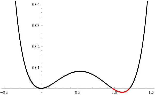
Since is locally convex near , is locally convex near , and so is one local minimum of . Subtracting off the tangent line function “tilts” the graph of downward to the right, and so the minimum of at gets tilted to a slightly negative value; the global minimum of lies in this dip below the axis. Since , the (negative) value of the global minimum is on the order of ; i.e., also . But since the curvature at the minimum is strictly positive, the width of the interval on which is negative is .
The following lemma makes this, and more, precise:
4.1 LEMMA.
Let be defined by (4.13). Then the equation has exactly three solutions, and where . There is a constant such that for all sufficiently large
| (4.16) |
and, if and only if . Consequently, if is any trial function with , and if is used in the definition of (4.1), and hence of , then is not empty.
Moreover, has a unique global minimizer which satisfies
for some fixed constant depending only on . If is any trial function with , there is an so that
is also a valid trial function with , and the sets , and determined by are the same as those determined by .
4.2 Remark.
The last part of this lemma says that if we seek to prove any theorem concerning the sets , and associated to a trial function with , then we may freely assume that is bounded above by . It also implies that any minimizer must be bounded above by .
Proof of Lemma 4.1: For the first part, we simply provide formulas that quantify the remarks in the paragraph preceding the statement of the lemma. It is clear from (4.13) that is one solution of . Also, since , and , it follows that for some ,
Thus, requires ; i.e., must lie in one of the two “wells” of . As before, let denote , the second derivative of at the bottom of the two wells. Let be defined by
Then on , and so
for . For large enough, , and so we may restrict our attention to values of in the intervals and . is strictly convex in both of these intervals, and since , is the unique minimizer of in the left interval.
To find the solutions in the right interval, introduce a new variable defined by and define . Then if and only if , and for such
| (4.17) | |||||
with in the second line. We have used the Taylor expansion and the fact that is even and is odd, and finally, the lower bound on in the well.
Evidently, unless where are the two roots of the quadratic expression on the right in (4.17). Since , it is evident that there is a constant such that
By the local convexity of , the remaining two solutions of must lie in the corresponding interval; i.e., , and is positive outside this interval. except at
When , is not constant, and . Hence, for , we must have on a set of positive measure. This proves the statements made in the first paragraph of the lemma.
To prove the claims made in the second paragraph, note that is an increasing function of to the right of its global minimum . Since truncation always lowers the interaction energy , replacing by lowers . Note that, if was not already bounded above by , the truncated function will no longer satisfy the constraint (4.11).
However, we can remedy this by another truncation at the other end: Let denote the positive and negative parts of . Then by (4.11),
and since
increases continuously from to as increases from to , we can choose so that
Since is a decreasing function of on , this second truncation also lowers , and restores the constraint (4.11). Finally, truncating at and , corresponds to a truncation in as in the lemma. The bound on comes from the fact that is the unique non-zero solution to
and what we have said in the proof of the first paragraph. ∎
4.3 Remark.
As mentioned in the introduction, our minimization problem is trivial for (and hence for by symmetry). This is easily seen by considering the functional used in the previous proof: If , then the tangent line being subtracted from the graph of in (4.13) would have a negative slope, and so subtracting it off would tilt the graph upward to the right, and not downward. Hence will have a unique global minimum at . Thus the unique minimizer of is the constant profile , and then by (4.14) the unique minimizer of is the constant profile . For the values and , the situation is even more elementary.
4.1 The bulk contribution
The key to estimating is that for small enough, is strictly convex on : For any , . Define the quantity by
Then, by Taylor’s Theorem, and using the fact that , we have
everywhere on .
Therefore,
| (4.18) | |||||
This estimate should be quite sharp, since we expect any nearly minimizing profile to be nearly constant in . Our problem is now reduced to that of estimating . Before going into the details, let us summarize what we would expect, and what lemmas we shall need, to prove what we would expect.
First, we would expect the transition region to be very “thin”, so that:
is negligible compared to and .
In that case, we would expect
| (4.19) | |||||
where in the last line, we have used the fact that is very close to on . In fact, on , by definition, and Lemma 4.1 and the remark following it will allow us to assume an upper bound of the form . Also, if is negligibly small,
| (4.20) |
Using (4.20) and (4.19), we would have . Then using (4.18) together with the simple (but not extravagant) bound , we would have
| (4.21) |
The next lemma gives the precise statement:
4.4 LEMMA.
Let be any trial function such that , and such that is bounded above by , where is defined and estimated in Lemma 4.1 . Then
with given by
| (4.22) |
for some constant .
4.5 Remark.
Note that if we choose , and if , then . The surface contribution will limit the side of , preventing cancelation in the main term, so that it will be , and hence strictly larger.
To prove Lemma 4.4 we first need to show that is in fact negligible, as explained in the heuristics. The following Lemma takes care of that:
4.6 LEMMA.
Let be any trial function such that . Then, for some finite and
Proof: We have
where , for some with and for small enough. It is easy to see from the definition of and the properties of the function that uniformly on ,
Therefore
On the other hand, since ,
Since , we get the result. ∎
Since and it is evident that ,
| (4.23) |
4.2 The surface contribution
Our goal in this subsection is to prove the following estimate.
4.7 LEMMA.
Let be any trial function such that ,
| (4.26) |
where is the surface tension, and , so that the bound is trivially true for , twice the range of .
Let us first explain the heuristics, and then collect the lemmas required to substantiate them. To prove this lemma we need to relate to the one dimensional functional defined in (3.1), which gives the planar surface tension . To do this, we use rearrangement inequalities to replace our near minimizer by a radial function on all of . This radial function will give us a trial function for (3.1).
The Riesz rearrangement inequality that we intend to use applies to functions on , and not on the torus, hence the first thing we have to do is to extend to a functional on profiles in all of without lowering the value of too much. Here is why we can expect that this is possible.
We expect that for a non-constant near minimizer , should be essentially a sphere of radius that we can take to be centered in , considered as a -cube of side length in , and that the whole transition region will be in an annulus close to . In particular, the truncation of that is defiend in (4.6) and used in the definition (4.9) of satisfies for all within unit distance of the boundary of the square. Now extend to a function on all of . Do this by defining for outside ; i.e.,
| (4.27) |
Then, since is supported by the unit sphere, it would follow from everywhere near the boundary of that
| (4.28) |
As for the potential term, define by
| (4.29) |
With this definition,
| (4.30) |
Then combing (4.9), (4.28) and (4.30), we would have
We are now in a position to use rearrangement inequalities to make contact with the one dimensional variational problem (3.1) that defines the planar surface tension: Let denote the spherical decreasing rearrangement of (see [23]). Then by the Riesz rearrangement inequality [23],
and of course
Therefore, if our intuition about the size and shape of is right, we should have
Let . Because of the spherical rearrangement, depends on , and the corresponding region is indeed a sphere of radius .
The key to making contact with the planar surface tension is the fact that , extended by for , is a valid trial function for the one dimensional variational problem (3.1) defining . We shall use this fact to get a lower bound on for a non-constant minimizer that is of the form (4.26). Note that apart from some small corrections, the main term in this bound is , the contribution we would expect for a droplet of radius .
To carry out this program of estimation, we need to show that is not too large: If is large, then it is easy for to “wrap around” so that (4.28) is not even approximately true. Then we would be prevented from applying the Riesz rearrangement inequality. Then next lemma shows that in fact, if is a trial function with , then , which we know to be non-empty by Lemma 4.1, has volume .
4.8 LEMMA.
Let be any trial function such that . Then, for sufficiently large, there is a constant such that
Proof: Since
| (4.31) |
we can use the obvious lower bounds on and on to conclude that
By using , we get
By Lemma 4.6, . Hence, for sufficiently large
On the other hand, by (4.18)
Therefore
by using .
Finally, using this in (4.31) we have:
Then
Using Lemma 4.6 to bound , and taking sufficiently large we conclude the proof.∎
Armed with this lemma on , we return to the proof of Lemma 4.7. In our heuristic discussion, we relied on our expectation that is nearly a disk centered in (with an appropriate choice of the origin in ) with a radius small compared to in order to justify (4.28). At this stage something less can be proved, which still suffices for the proof of Theorem 2.1:
If is a trial function with , and if does “wrap around the torus” , then the arms that “wrap around” are very thin, as shown in Figure 2.

For any of the coordinate directions , consider the volume of that is contained in the slab . If for each choice of this volume is at least , then
since integrating this volume in from to gives twice the volume of . Hence there is at least one choice of for which
Now by the translation invariance of , we may freely translate , and so may assume that . Thus without loss of generality, we may assume that for each coordinate direction ,
| (4.32) |
4.9 LEMMA.
There is a constant so that for any trial function with ,
and for some finite ,
Proof: The integral on the left hand side can only be smaller than the integral on the right hand side only on account of pairs of points with, say, in the cube representing , and outside it, and where , since otherwise . Since has unit range, must have for at least one . Hence the total contribution from such pairs of points is a fixed multiple of , by (4.32). Then using our bounds on and from Lemmas 4.6 and 4.8, we obtain final bound. ∎
Lemma 4.9 gives us the rigourous replacement for (4.28) in our heuristic analysis. We now turn to the term involving . Note that at all points in the support of . Hence, going to spherical coordinates,
| (4.33) |
Therefore, if , then
| (4.34) |
for all , since has unit range.
Hence by (3.9),
| (4.35) |
where once again, is the positive part function. Indeed, the left hand side is clearly positive, so if is sufficiently small that using the uniform bound on the Jacobian that led to (3.9) provides a negative lower bound, simply use the trivial lower bound by zero instead.
Next, since (4.34) implies for all , we have
| (4.36) |
We are now ready to prove Lemma 4.7:
Proof of Lemma 4.7: By (4.30) and (4.33) for the terms involving , and Lemma 4.9 and (4.36), it remains only to show that
Our proof of this rests on the fact that , extended by for , is a valid trial function for the variational problem defining . To show this, we need to prove that it approaches the correct asymptotic values; i.e., that it satisfies the constraint imposed on (3.1). In fact, due to the lemma 4.1, in not empty when , and of course is not empty too. So, by the definition of , for all . Consequently, if so that provided , the range of we can extend the region of integration to :
| (4.37) |
Now, if , the bound in the Lemma is trivial, and there is nothing to prove, Hence there is no harm in assuming that , which we now do.
Since is decreasing on , and since for , , it follows that
Therefore,
| (4.38) | |||||
The proof of Lemma 4.7 is complete. ∎
5 Proofs of the theorems.
5.1 Proof of the Theorem 2.1
We fix the value for the proof. Given a trial function with , we replace by its truncation as defined in Lemma 4.1. This lowers the free energy, and does not change the sets , and . In summary, after this replacement we have a trial function that has a free energy at least as low as the one we started with, the same value of , and which is bounded above by as in Lemma 4.1.
Then using Lemmas 4.7 and 4.4 we conclude that
It now remains to optimize this over . We note that the lower bound on decreases as increases until is of order . But for such values of , the expression for the lower bound on the surface contribution simplifies:
Now introduce and . Then we can rewrite this lower bound as
| (5.2) |
By Lemma 4.6, , and by Lemma 4.8, . Thus, . Therefore,
With the choice , this gives us , as noted in the remark following Lemma 4.4. The essential point is that this is negligible compared to as tends to infinity in the critical scaling regime.
As in the critical scaling regime, and . Moreover, from (4.5) and the definition of , as . Thus, (5.2) provides the lower bound needed to prove (2.13). The upper bound is provided by Lemma 3.1. The remaining statements follow from the analysis of the minimization of the phenomenological free energy function that was explained in Section 2 ∎
5.2 Proof of Theorem 2.2
Suppose that where . We shall show that, in this case, any non-constant trial function has a higher free energy than the uniform trial function , at least for all sufficiently large .
Recalling that , define by
As in the proof of Theorem 2.1, for all sufficiently large, is sufficiently close to , and is sufficiently close to that
for some . For , the unique minimizer of
is . Therefore, since as , it follows that as .
Now, as in the previous section, for any non-uniform minimizer , there is a relation between and the size of the level set : for a given , . Here, as in the last section, with given by (4.5). It follows from (5.2) and the definition of that for any non-constant minimizer , , and so is negligibly small compared with , the volume of the equimolar ball, when is large.
In other words, if where , and is large, then any droplet in any minimizer must be extremely small. To prove Theorem 2.2, it therefore suffices to show that such extremely small drops are impossible in a minimizing . The following Lemma gives the required lower bound, and completes the proof. ∎
5.1 LEMMA.
For all , there is a constant depending only on so that if and is any non-uniform minimizer for (1.1), then
Moreover, is uniformly strictly positive for all in an interval around .
We first explain the idea behind the proof. It is convenient to use (4.14) to write in terms of as in the proof of Lemma 4.1.
We know from Lemma 4.1, using the notation from there, that if , then . Since for some , for all , and since the set on which is contained in ,
| (5.3) |
Now, if we could show that for some ,
we would have
and this is strictly positive unless is on the order of , and in the critical scaling regime, is proportional to .
Of course
| (5.4) |
so we can hope to bring the methods of Section 4.3 to bear on this problem. There are two obstacles: The first obstacle is that the possible penalty for “unwrapping the torus” that is estimated in Lemma 4.9 is of order . When is small, so is , but the only upper bound that we have on is the one provided by Lemma 4.6. This is independent of , and so it very well can be that for small , is large compared to , so that the penalty for “unwrapping the torus” completely swallows up the surface term.
The second obstacle is that lower bound on the surface contribution that we obtained in Lemma 4.7 becomes trivial for , twice the range of .
To deal with the first obstacle, use the fact that on , for some . Therefore,
We then have from (5.4) that
| (5.5) |
Since
for all large , the final term in (5.5) more than compensates for the price of “unwrapping the torus”.
It remains to deal with the second obstacle, as concerns
Toward this end, we first give a simple, direct argument, independent of the reasoning in Section 4.3 to show that if , and is not constant, then is bounded below by a constant of order one. Specifically, we shall show that in this case , .
We then “cut down” the range of so this it is small compared with . That is, for , define for , and otherwise. Having reduced the range of , the error term in (3.9) becomes for . We choose sufficiently small that this factor is at least for . This shall take care of the second obstacle. We now provide the detials.
Proof of Lemma 5.1: We shall first show that if , and is not constant, then . First of all, by Lemma 4.1, if , and is not constant, then is not empty, and at least we know . Let us improve on this.
With defined as in Lemma 4.1, define , and define so that . Then by Lemma 4.1, there is a constant so that .
We now claim that if , the interaction term makes a much larger positive contribution to , so that , which would imply .
Now, by our assumptions on , for each , on the ball of radius about . If , then can fill up at most one half of this ball, and so the volume of the set of points in the ball of radius about for which is at least . Hence
for some . Altogether, , and this is strictly positive for large enough. Therefore, we may assume without loss of generality that is such that .
We return to (5.5), and “cut down” the range of , replacing by , , which clearly decreases the right hand side of (5.5)
| (5.6) |
Now let be defined in terms of just as is defined in terms of , and let denote the the rearrangement of , as before. Having reduced the range of from to , the estimate (4.36) becomes
| (5.8) |
where once again, is the positive part function.
We now choose small enough that the prefactor is at least for . Of course, we also have
| (5.9) |
where as in (4.29), we define by
| (5.10) |
Now let be defined by
| (5.12) |
5.3 Proof of Theorem 2.3.
Suppose is such that , for some given . With the notation of the previous sections, let and be the optimal volume fraction corresponding to . Then, by (5.2) we get
| (5.13) | |||||
This entails that . By the definition of , there is a constant such that , so, for sufficiently large .∎
6 The shape problem
Throughout this section, we use the notation defined in (4.1) and (4.2). In particular, given a trial function , the set is the set of points on which takes values that are close to or larger, is the set of points on which takes values that are close to or smaller, and is everything else. We shall also assume that is defined on all of ; we have already seen how to extend from to with negligible cost in free energy, so let us suppose this is done, and and are finite. Finally, in this subsection we use the notation (4.3), so that is the radius of the ball in with the same Lebesgue measure as . Up to now, we have been concerned with the sizes of and . Going forward, we are concerned with their shape. It is easier to get control of this in the local case.
In the case of the local (Allen-Cahn or van der Waals) free energy functional (1.9), the lower bound (1.1) brings the surface area of the boundary of into the lower bound on the free energy. Then stability results for the isoperimetric inequality [7, 19, 20] can be used to show [11] that if is not nearly spherical, there is a significant cost in free energy. It is an open problem, which we refer to as the shape problem, to prove this for the Gates-Lebowitz-Penrose free energy functional. To clarify the difference between the local and non-local cases, let us briefly recall an argument from [11]. (We shall in fact improve the result in [11] by using a new stability inequality from [16].)
Let be a Borel measurable set in . As usual, let denote is Lebesgue measure, and let denote its perimeter. If the set is sufficiently regular, is the dimensional Haussdorf measure of the boundary of , though for very irregular sets it can be much smaller. The perimeter functional is an extension of the surface area functional to general Borel sets, due to De Giorgi [13] , with the key property that it enjoys good lower semicontinuity properties. See Maggi’s review [26] for more information.
The isoperimetric deficit of , , is the quantity
| (6.1) |
The general isoperimetric inequality of De Giorgi says that with equality if and only if , up to a set of measure zero, is a ball.
The stability results that we refer to give a lower bound on in terms of the Fraenkel asymmetry of , , which measures the extent to which differs from being a ball:
| (6.2) |
where is the ball of radius centered on in , and denotes the symmetric difference of and ; that is,
The theorem of Fusco, Maggi and Pratelli [16] says that for all , there is a constant depending only on , so that for all Borel sets in ,
| (6.3) |
This improved on an earlier result of Hall, Hayman and Weitsman [19, 20] of the same character, but with in place of . The exponent is sharp; see [26] for further discussion and background.
To apply this result to the shape problem for the local free energy functional, suppose that for some trial function and some , one has that the volume of lying outside every ball of radius is at least .
Now let be defined by
so that , and . By containment, if , then . This has the consequence that for all , the volume of lying outside every ball of radius is at least .
Moreover, since in the critical scaling regime, Lemma 4.6 says that is negligible compared to , for all sufficiently large , and all , the radius of a ball in with the same volume as is no greater than .
Consequently, for each , . Therefore, by (6.3), and one more use of ,
In the context of (1.1), for almost every , , the dimensional Haussdorf measure of the set , and hence we have a lower bound on that is uniform in . Using this in (1.1), one gets a lower bound on the free energy of that is larger than the minimizing value by a factor of (essentially) . Hence if the free energy of a trial function is sufficiently close to the minimizing value, must be correspondingly small. This forces to be very nearly a ball. A similar argument applies to each of the for , although the degree of control on the roundness of diminishes as approaches . A precise statement in terms of the distance between and an ideal round droplet profile may be found in [11].
It is an interesting open problem to develop bounds of this type that would apply to the Gates-Lebowitz-Penrose free energy functional. It would be very surprising if the physical model behind it did not capture enough physical reality to control the shape of droplets in near-minimizers. We note that one can apply stability for the isoperimetric inequality to the GLP functional, but only in the sharp interface scaling limit, as discussed in [30]. However the size of our critical droplet goes to zero in this limit.
What would seem to be useful here would be a stability result for the Riesz rearrangement inequality, or at least the special case in which one of the three functions is already rearranged, and has all centered balls of sufficiently small radius as level sets. A general stability result for it might be quite subtle; the cases of equality were only determined relatively recently by Burchard [8]. However, for is radially symmetric and well-behaved, there is a simpler and cleaner result on the cases of equality due to Lieb [22], and in this setting, one might expect a stability result that would force the other two functions to be nearly rearranged for near minimizers. This will be the subject of future research.
Acknowledgments
We would like to thank Thierry Bodineau and Errico Presutti for very helpful discussions. E. C. was partially supported by U.S. NSF grant DMS 06-00037. M.C.C. was partially supported by undao para a Cincia e a Tecnologia, Financiamento Base 2008 - ISFL/1/209 and grant POCI/MAT/61931/2004. R.M. and R. E. were partially supported by MIUR, INDAM-GNFM. J.L.L. was supported by AFORS grant AF 49620-01-1-0154 and NSF Grant DMR-044-2066. This work has also been supported by the European Commission through its 6th Framework Program “Structuring the European Research Area” and the contract Nr. RITA-CT-2004-505493 for the provision of Transnational Access implemented as Specific Support Action.
References
- [1] Alberti G., Bellettini G., Cassandro M. and Presutti E., Surface Tension in Ising Systems with kac Potentials, J.Stat.Phys, 82, 743–796 (1996).
- [2] G. Bellettini, M. S. Gelli, S. Luckhaus and M. Novaga, Deterministic equivalent for the Allen-Cahn energy of a scaling law in the Ising model, Calc. Var. P.D.E., 26 no. 4, 429–445, (2006).
- [3] T. Bodineau and E. Presutti, Phase diagrams of Ising systems with additional long range forces, Commun. Math. Phys., 189, No. 2, 287–298, (1997).
- [4] O. Benois, T. Bodineau and E. Presutti, Large deviations in the van der Waals limit, Stochastic Process. Appl. 75, 89–104, (1998).
- [5] M. Biskup, L. Chayes, R. Kotecky, On the formation/dissolution of equilibrium droplets, Europhys. Lett. 60, 21– 27, (2002).
- [6] M. Biskup, L. Chayes, R. Kotecky, Critical Region for Droplet Formation in the Two-Dimensional Ising Model, Comm. Math. Phys., 242, 137– 183, (2003).
- [7] Bonnesen, T., Über eine Verschärfung der isoperimetrischen Ungleichheit des Kreises in der Ebene und auf der Kugeloberfläche nebst einer Anwendung auf eine Minkowkische Ungleichheit für konvexe Körper, Math. Annalen 84, 216–227, (1921). Über die Isoperimtrische Defizit ebener Figuren, Math. Ann., 91, 252-268 (1924).
- [8] A. Burchard, Cases of equality in the Riesz rearrangement inequality, Annals of Math. 143, 499-527, (1996).
- [9] E.A. Carlen, M. Carvalho , R. Esposito, J. L. Lebowitz and R. Marra , Free Energy Minimizers for a Two–Species Model with Segregation and Liquid-Vapor Transition, Nonlinearity 16, 1075–1105 (2003).
- [10] E.A. Carlen, M. Carvalho , R. Esposito, J. L. Lebowitz and R. Marra, Molecular Physics 103 (2005), 3141Ð3151 Phase transitions in Equilibrium Systems: Microscopic Models and Mesoscopic Free Energies, Molecular Physics 103, 3141Ð3151 (2005).
- [11] E. Carlen, M. C. Carvalho, R. Esposito, J. L. Lebowitz and R. Marra, Droplet minimizers for the Cahn–Hilliard free energy functional, J. Geometric Analysis 16, 233–264, (2006).
- [12] J. de Boer, Van der Waals in His Time and The Present Revival - Opening Address, in Van der Waals Centennial Conference on Statistical Mechanics, Amsterdam, 27-31 August 1973, C. Prins, editor, North-Holland, Amsterdam, 1-17, (1974).
- [13] E. De Giorgi, Su una teoria generale della misura -dimensionale in uno spazio ad dimensione, Ann. Mat. Pura Appl. 36, 1191-213, (1954). Nuovi teoremi relativi alle misure -dimensionali in uno spazio ad dimensione, Ricerche Mat., 4, 95-113, (1955). Sulla proprietà isoperimetrica dell’ipersfera, nella classe degli insiemi aventi frontiera orientata di misura finita, Atti Accad. Naz. Lincei. Mem. Cl. Sci. Fis. Mat. Nat. Sez. I 5 , 33-44, (1958).
- [14]
A. De Masi, E. Orlandi, E. Presutti and L. Triolo:
Stability of the interface in a model of phase separation, Proc. Royal Soc. Edinburgh, 124 (1994). - [15] H. Federer, Geometric Measure Theory, Springer-Verlag, Berlin, 1969.
- [16] N. Fusco, F. Maggi, A. Pratelli, The sharp quantitative isoperimetric inequality, to appear in Ann. of Math.
- [17] G.B. Giacomin and J.L. Lebowitz, Phase segregation dynamics in particle systems with long range interactions II: interface motions SIAM J. Appl.Math. 58 1707–1729 (1998).
- [18] Gates D.J. and Penrose O., The van der Waals limit for classical systems. I. A variational principle. Commun. Math. phys. 15 255–276 (1969).
- [19] R. Hall, A quantitative isoperimetric inequality in n dimensional space, J. d’Analyse Math., 56, 87-123, (1992).
- [20] R. Hall, W. Hayman and A. Weitsman, On asymmetry and capacity, J. Reine angew. Math 428, 61–76, (1991).
- [21] M. Kac, G.Uhlenbeck, P.C.Hemmer, On the van der Waals theory of vapor-liquid equilibrium. I. Discussion of a one dimensional model, J. Math. Phys. 4, 216–228, (1963); II. Discussion of the distribution functions, J. Math. Phys. 4, 229–247 (1963); III.Discussion of the critical region,J. Math. Phys. 5, 60Ð74, (1964).
- [22] E. H. Lieb, Existence and uniqueness of the minimizing solution of Choquard’s nonlinear equation. Studies in Applied Mathematics, 57, 93–105 (1977).
- [23] E. H. Lieb, M. Loss, Analysis. Graduate Studies in Mathematics, vol. 14, American Mathematical Society, Providence (2001).
- [24] S Luckhaus and L. Modica, The Gibbs-Thompson relation within the gradient theory of phase transitions Archive for Rat. Mech. Analysis 107 71–83, (1989).
- [25] Lebowitz J.L. , Penrose O., Rigorous treatment of the Van der Waals Maxwell theory of the liquid vapor transition J. Math. Phys., 7, 98, (1966).
- [26] F. Maggi, Some methods for studying stability in isoperimetric type problems, Bull. A. M. S. 45, no. 3, 367–408, (2008).
- [27] L. Modica, The gradient theory of phase transitions and the minimal interface criterion, Arch. Rat. Mech. Analysis 98, 123–142, (1987)
- [28] L. Modica and S. Mortola, Un esempio di –convergenza, Boll. Un. Mat. Ital., 5, 285–289, (1977)
- [29] R. Osserman, Bonnesen-style isoperimetric inequalities, Am. Math. Monthly 86 1–29,(1972)
- [30] E. Presutti Scaling Limits in Statistical Mechanics and Microstructures in Continuum Mechanics Springer (2008)
- [31] J. S. Rowlinson and B. Widom, Molecular Theory of Capillarity, Oxford University Press, Oxford, 1982
- [32] J. D. van der Waals, Théorie moléculaire d’une substance composée de deux matières différentes, I Verhandelingen, Kon. Akad. Wet. Amsterdam 20 (1880) and Théorie moléculaire d’une substance composée de deux matières différentes, II, Arch. néerl. 24, 1 (1891).