Lyapunov Analysis of Homogeneous Isotropic Turbulence

This work presents a study of isotropic and homogeneous turbulence for an incompressible fluid in an infinite domain. The analysis is mainly motivated by the fact that in turbulence the kinematics of the fluid deformation is subjected to bifurcations [1] and exhibits a chaotic behavior and huge mixing [2], resulting to be much more rapid than the fluid state variables. This characteristics implies that the accepted kinematical hypothesis for deriving the Navier-Stokes equations could require the consideration of very small length scales and times for describing the fluid motion [3] and therefore a very large number of degrees of freedom.
Other peculiar characteristics of the turbulence are the mechanism of the kinetic energy cascade, directly related to the relative motion of a pair of fluid particles [4, 5, 6, 7] and responsible for the shape of the developed energy spectrum, and the non-gaussian statistics of the velocity difference.

The present analysis assumes that the fluctuations of all the fluid state variables are the result of the bifurcations of the velocity field. The evolution in the time of these fluctuations is calculated with the Lyapunov analysis of the particle equations of motion.

The first part of the work deals with the representation of velocity difference between two fixed points of the space. This is analyzed with the Lyapunov theory studying the motion of the particles crossing the two points. This analysis gives an explanation of the mechanism of kinetic energy transfer between length scales and leads to the closure of the von Kármán-Howarth equation [6]. The obtained expression of the function $K(r)$, which represents the inertia forces, is in terms of the longitudinal correlation function and its spatial derivative, and satisfies the conservation law which states that the inertia forces only transfer the kinetic energy [6, 7].

In the second part, the statistics of the velocity difference is studied through the kinematics of the local deformation and the momentum equations. These momentum equations are expressed with respect to the referential coordinates which coincide with the material coordinates for a given fluid configuration [3], whereas the kinematics of the local deformation is analyzed with the Lyapunov theory. The choice of the referential coordinates allows the velocity fluctuations to be analytically expressed in terms of the Lyapunov exponent of the local fluid deformation. The statistics of velocity difference is studied with the Fourier analysis of the velocity fluctuations, and an analytical expression for the velocity difference and for its PDF is obtained in case of isotropic turbulence. This expression incorporates an unknown function, related to the skewness, which is identified through the obtained expression of $K(r)$. The velocity difference also requires the knowledge of the critical Reynolds number whose estimation is made in the Appendix B, where the order of magnitude is roughly determined through a qualitative analysis of the bifurcations of the velocity field.

Finally, the several results obtained with this analysis are compared with the data existing in the literature, indicating that the proposed analysis can adequately describe the various properties of the fully developed turbulence.

The present analysis only studies the possibility to obtain the fully developed homogeneous-isotropic turbulence in a given condition and does not analyze the intermediate stages of the turbulence.

In order to investigate the mechanism of the energy cascade, the properties of the relative equations of motion between fluid particles are here studied with the Lyapunov analysis. To this purpose, consider two fixed points of the space, ${\bf X}$ and ${\bf X}^{\prime}$ (see Fig. 1) whose distance is $r=|{\bf X}^{\prime}-{\bf X}|$ and the motion of two fluid particles which at a given time $t_{0}$, cross through ${\bf X}$ and ${\bf X}^{\prime}$. The equations of motion of these particles are

At $t_{0}$, a toroidal volume $\Sigma(t_{0})$ is chosen which contains ${\bf X}$ and ${\bf X}^{\prime}$, whose geometry and position change according to the fluid motion. In Fig. 1, $S_{p}\gtrapprox r^{2}$ and $R$ are, respectively, the poloidal surface and the toroidal dimension of $\Sigma$ which vary with time to preserve the volume. The velocity difference associated to ${\bf X}$ and ${\bf X}^{\prime}$ is $\Delta{\bf u}={\bf u}({\bf X^{\prime}},t)-{\bf u}({\bf X},t)$ and its components $\Delta u_{n}\equiv u_{n}^{\prime}-u_{n}$ and $\Delta u_{r}\equiv u_{r}^{\prime}-u_{r}$, lay on $S_{p}$ and are normal and parallel to $r$, respectively, whereas $u_{b}$ is the average of the velocity components along the direction normal to $S_{p}$. According to the theory [8], for $t>t_{0}$, the trajectories of the two particles are enclosed into $\Sigma(t)$. For sake of simplicity and without loss of generality, we assume that $R$ increases with time [8]. The Lyapunov analysis of Eqs. (II) leads to

These variations of $R$ are caused of the bifurcations [8] of Eqs. (II). Since $R$ rises with time, $\lambda(r)>$ 0 identifies the maximal finite scale Lyapunov exponent associated to Eqs. (II).

The equations of motion for $\displaystyle\Sigma(t)$ preserve the volume and can be expressed in terms of the velocity components calculated at $\bf X$ and $\bf X^{\prime}$ [9]. These are

In line with Lamb [9], Eqs (II) and (II) represent, respectively, the continuity equation and the momentum equations which can be derived from the integral equations of balance over $\Sigma$. Into Eq.(II), $\nu$ is the kinematic viscosity, $\beta=O(1)>0$ is a proper constant, and $J$ is related to the time derivative of the kinetic energy and to the viscosity [9]. $J$ is equal to zero when $\nu=$ 0.

Equations (II) and (II) are written in terms of the fluid properties calculated at $\bf X$ and $\bf X^{\prime}$, thus are referred to the Eulerian description of motion [3, 9]. Substituting Eq. (3) into Eqs. (II) and (II), one obtains

Since $\lambda>0$, $u_{b}\rightarrow 0$. Equations (II) describe fluctuations of velocity difference caused by bifurcation of Eqs. (II) and hold as long as $\bf X$ and $\bf X^{\prime}$ are both enclosed into $\Sigma(t)$. This condition is verified if $t-t_{0}$ does not exceed very much the order of magnitude of $1/\lambda$ [8].

In order to obtain the closure of the von Kármán-Howarth equation, Eq. (II) enter the computation of the average of the physical quantity $\Upsilon$:

where $T_{ij}$ = $\displaystyle-{p}\delta_{ij}+\nu\rho\left({\partial u_{i}}/{\partial x_{j}}+{\partial u_{j}}/{\partial x_{i}}\right)$ is the stress tensor. The repeated indexes denote the summation with respect to the same indexes, which are $i$ = $r,n,b$ and $j$ = $r,n,b$.

According to von Kármán [6], $\Upsilon$ expresses that part of the inertia forces, responsible for the transferring of the kinetic energy between the several fluid regions, whose average only depends on the current value of the average kinetic energy. In the von Kármán-Howarth equation, the function $K(r)$ is the average of $\Upsilon$. The average is calculated on all the pairs of particles which cross through ${\bf X}$ and ${\bf X}^{\prime}$ at the same time. Specifically, $K(r)$ is determined substituting Eqs. (II) into Eq. (16), assuming the homogeneity and the isotropy and taking into account that $\langle\Upsilon\rangle$ does not depend neither on $\partial\langle u_{i}u_{i}\rangle/\partial t$, nor on $\langle{\partial T_{ij}}/{\partial x_{j}}u^{\prime}_{i}+{\partial T^{\prime}_{ij}}/{\partial x^{\prime}_{j}}u_{i}\rangle$ [6, 7]. This immediately identifies

where $u^{2}=\langle u_{i}u_{i}\rangle/3$ and $f$ and $g$ are longitudinal and lateral velocity correlation functions. Due to the fluid incompressibility, $f$ and $g$ are related each other through $g=f+1/2\partial f/\partial r$ (see Eq. (78), Appendix A), leading to the expression

Considering that $K(r)$ does not directly depend on the viscosity, this expression can be also obtained at $\nu$ = 0. In this case $\langle J\rangle$ = 0, $\partial\langle u_{i}u_{i}\rangle/\partial t$ = 0, $\langle{\partial T_{ij}}/{\partial x_{j}}u^{\prime}_{i}+{\partial T^{\prime}_{ij}}/{\partial x^{\prime}_{j}}u_{i}\rangle$ = 0 [6], and Eqs. (II) and (21) are again recovered.

Equation (21) states that, the fluid incompressibility, expressed by $g-f\neq 0$, represents a sufficient condition to state that $K(r)\neq$ 0. This latter is determined as soon as $\lambda$ is known. To calculate $\lambda$, it is convenient to express $\Delta{\bf u}={\bf u}({\bf X}^{\prime},t)-{\bf u}({\bf X},t)$ in the Lyapunov basis of orthonormal vectors $E\equiv({\mbox{\boldmath$\varepsilon$}}_{1},{\mbox{\boldmath$\varepsilon$}}_{2},{\mbox{\boldmath$\varepsilon$}}_{3})$ associated to Eqs. (II) [10, 11]. The velocity difference expressed in $E$, $\Delta{\bf v}\equiv(v_{1}^{\prime}-v_{1},\ v_{2}^{\prime}-v_{2},\ v_{3}^{\prime}-v_{3})$, satisfies the following equations, which hold for times whose order of magnitude do not exceed very much $1/{\lambda}$ [8, 12]

where $\hat{r}_{i}$, $v_{i}$ and $v_{i}^{\prime}$ are, respectively, the components of ${\bf X}^{\prime}-{\bf X}$, ${\bf u}({\bf X},t)$ and ${\bf u}({\bf X}^{\prime},t)$ written in $E$. Then, $r$ and $\Delta u_{r}$ can be expressed in terms of $\hat{\bf r}$ and $\Delta{\bf v}$ as

Into Eqs. (II), ${\bf Q}\equiv((\varepsilon_{ij}))$ is the rotation matrix transformation from $E$ to $\Re$, where $\varepsilon_{ij}$ is the component of ${\mbox{\boldmath$\varepsilon$}}_{j}$ along the coordinate direction $i$ on $\Re$, and ${\mbox{\boldmath$\xi$}}=({\bf X}^{\prime}-{\bf X})/|{\bf X}^{\prime}-{\bf X}|$.

The standard deviation of $\Delta u_{r}$ is calculated from Eqs. (II), taking into account that $\Delta{\bf v}\approx\lambda\hat{\bf r}$ and that $\bf Q$ is fluctuating depending on the pair paths:

Since $\lambda$ is calculated as the average of the velocity increment per unit distance, it is constant with respect the statistics of $\varepsilon_{ij}$ and $\varepsilon_{pq}$ [11], thus $\langle{\lambda}^{2}\varepsilon_{ij}\varepsilon_{pq}\rangle={\lambda}^{2}\langle\varepsilon_{ij}\varepsilon_{pq}\rangle$. Furthermore, due to isotropy, the Lyapunov vectors fluctuate in such a way that $\langle\varepsilon_{ij}\varepsilon_{pq}\rangle=\delta_{ij}\delta_{pq}$[11]. As the result, the standard deviation of the longitudinal velocity difference is

This standard deviation can be also expressed through the longitudinal correlation function $f$

being $u$ the standard deviation of the longitudinal velocity. The maximal Lyapunov exponent is calculated in function of $f$, from Eqs. (27) and (28)

Hence, substituting Eq. (29) into Eq. (21), one obtains the expression of $K(r)$ in terms of the longitudinal correlation function

Thanks to the isotropy, $K(r)$ is a function of $r$ alone.

Equation (30) represents the proposed closure of the von Kármán-Howarth equation. This is the consequence of the fact that, the kinetic energy, initially enclosed into $\Sigma(t_{0})$, at the end of the fluctuation is contained into $\Sigma(t)$ whose dimensions are changed with respect to $\Sigma(t_{0})$ in agreement with the Lyapunov theory. This corresponds to a mechanism of the kinetic energy transferring between diverse regions of space which preserves the average values of the momentum and of the kinetic energy. Specifically, the analytical structure of Eq.(30) states that this mechanism consists of a flow of the kinetic energy from large to small scales which only redistributes the kinetic energy between wavelengths.

The obtained expression of $K(r)$ allows to determine the skewness of $\Delta u_{r}$ [7]

which is expressed in terms of the longitudinal triple correlation $k(r)$, linked to $K(r)$ by $K(r)=u^{3}\left({\partial}/{\partial r}+4/r\right)k(r)$ (also see Appendix A, Eq. (81)). Since $f$ and $k$ are, respectively, even and odd functions of $r$ with $f(0)$ = 1, $k(0)=k^{\prime}(0)=k^{\prime\prime}(0)$ =0, $H_{3}(0)$ is given by

where the apex denote the derivative with respect to $r$. To obtain $H_{3}(0)$, observe that, near the origin, $K$ behaves as

then, substituting Eq. (III) into $K(r)=u^{3}\left({\partial}/{\partial r}+4/r\right)k(r)$ and accounting for Eq. (32), one obtains

This value of $H_{3}(0)$ is a constant of the present analysis, which does not depend on the Reynolds number. This is in agreement with the several sources of data existing in the literature such as [7, 13, 14, 15] (and Refs. therein) and its value gives the entity of the mechanism of energy cascade.

As explained in this section, the Lyapunov analysis of the local deformation and some plausible assumptions about the statistics of velocity difference $\Delta{\bf u}({\bf r})\equiv{\bf u}({\bf X}+{\bf r})-{\bf u}({\bf X})$ lead to determine all the statistical moments of $\Delta{\bf u}({\bf r})$ with only the knowledge of the function $K(r)$ and of the value of the critical Reynolds number.

Starting from the momentum Navier-Stokes equations

consider the map $\chi$ : ${\bf x}_{0}\rightarrow{\bf x}$, which is the function that determines the current position $\bf x$ of a fluid particle located at the referential position ${\bf x}_{0}$ [3] at $t=t_{0}$. Equation (36) can be written in terms of the referential position ${\bf x}_{0}$ [3]

The Lyapunov analysis of the fluid strain provides the expression of this deformation in terms of the maximal Lyapunov exponent

where $\Lambda\equiv\lambda(0)=\max(\Lambda_{1},\Lambda_{2},\Lambda_{3})$ is the maximal Lyapunov exponent and $\Lambda_{i}$, $(i=1,2,3)$ are the Lyapunov exponents. Due to the incompressibility, $\Lambda_{1}+\Lambda_{2}+\Lambda_{3}=$ 0, thus, $\Lambda>0$.

If we assume that this deformation is much more rapid than ${\partial T_{kh}}/{\partial x_{0p}}$ and ${\partial{u}_{k}}/{\partial x_{0p}}u_{h}$, the velocity fluctuation can be obtained from Eq. (37), where ${\partial T_{kh}}/{\partial x_{0p}}$ and ${\partial{u}_{k}}/{\partial x_{0p}}u_{h}$ are supposed to be constant with respect to the time

This assumption is justified by the fact that, according to Truesdell [3], ${\partial T_{kh}}/{\partial x_{0p}}-{\partial{u}_{k}}/{\partial x_{0p}}u_{h}$ is a smooth function of time -at least during the period of a fluctuation- whereas the fluid deformation varies very rapidly in proximity of a bifurcation according to Eq. (38).

The statistical properties of $\Delta{\bf u}({\bf r})$, are investigated expressing the velocity fluctuation, given by Eq. (IV), as the Fourier series

where ${\bf U}({\mbox{\boldmath$\kappa$}})$ $\equiv$ $(U_{1}({\mbox{\boldmath$\kappa$}}),U_{2}({\mbox{\boldmath$\kappa$}}),U_{3}({\mbox{\boldmath$\kappa$}}))$ are the components of velocity spectrum, which satisfy the Fourier transformed Navier-Stokes equations [7]

All the components ${\bf U}({\mbox{\boldmath$\kappa$}})\approx\partial{\bf U}({\mbox{\boldmath$\kappa$}})/{\partial t}/\Lambda$ are random variables distributed according to certain distribution functions, which are statistically orthogonal each other [7].

Thanks to the local isotropy, $\bf u$ is sum of several dependent random variables which are identically distributed [7], therefore $\bf u$ tends to a gaussian variable [16], and ${\bf U}({\mbox{\boldmath$\kappa$}})$ satisfies the Lindeberg condition, a very general necessary and sufficient condition for satisfying the central limit theorem [16]. This condition does not apply to the Fourier coefficients of $\Delta{\bf u}$. In fact, since $\Delta{\bf u}$ is the difference between two dependent gaussian variables, its PDF could be a non gaussian distribution function. In ${\bf x}=0$, the velocity difference $\Delta{\bf u}({\bf r})\equiv(\Delta u_{1},\Delta u_{2},\Delta u_{3})$ is given by

This fluctuation consists of the contributions appearing into Eq. (IV): in particular, $L$ represents the sum of all linear terms due to the viscosity and $B$ is the sum of all bilinear terms arising from inertia and pressure forces. $P$ and $N$ are, respectively, the sums of definite positive and negative square terms, which derive from inertia and pressure forces. The quantity $L+B$ tends to a gaussian random variable being the sum of statistically orthogonal terms [17, 16], while $P$ and $N$ do not, as they are linear combinations of squares [17]. Their general expressions are [17]

where $P_{0}$ and $N_{0}$ are constants, and $\eta_{1}$, $\eta_{2}$, $\zeta_{1}$ and $\zeta_{2}$ are four different centered random gaussian variables. Therefore, the fluctuation $\Delta u_{r}$ of the longitudinal velocity difference can be written as

where $\xi$, ${\eta}$ and $\zeta$ are independent centered random variables which have gaussian distribution functions with standard deviation equal to the unity. The parameter $\chi$ is a positive definite function of Reynolds number, whereas $\psi_{1}$ and $\psi_{2}$ are functions of space coordinates and the Reynolds number.

At the Kolmogorov scale $\ell$, the order of magnitude of the velocity fluctuations is ${u_{K}}^{2}\tau/\ell$, with $\tau=1/\Lambda$ and $u_{K}=\nu/\ell$, whereas $\psi_{2}$ is negligible because is due to the inertia forces: this immediately identifies $\psi_{1}\approx{u_{K}}^{2}\tau/\ell$.
On the contrary, at the Taylor scale $\lambda_{T}$, $\psi_{1}$ is negligible and the order of magnitude of the velocity fluctuations is $u^{2}\tau/\lambda_{T}$, therefore $\psi_{2}\approx u^{2}\tau/\lambda_{T}$.

The ratio $\psi_{2}/\psi_{1}$ is a function of $R_{\lambda}$

where $\displaystyle\hat{\psi}({\bf r})=O(1)$, is a function which has to be determined.

Hence, the dimensionless longitudinal velocity difference $\Delta{u}_{r}$, is written as

The dimensionless statistical moments of $\Delta{u}_{r}$ are easily calculated considering that $\xi$, $\eta$ and $\zeta$ are independent gaussian variables

where

In particular, the third moment or skewness, $H_{3}$, which is responsible for the energy cascade, is

For $\chi\neq$ 1, the skewness and all the odd order moments are different from zero, and for $n>3$, all the absolute moments are rising functions of $R_{\lambda}$, thus $\Delta u_{r}$ exhibits an intermittency whose entity increases with the Reynolds number.

All the statistical moments can be calculated once the function $\chi(R_{\lambda})$ and the value of $\hat{\psi}_{0}$ are known. The expression of $K(r)$ obtained in the first part of the work allows to identify $H_{3}(0)$ and then fixes the relationship between $\psi_{0}$ and $\chi(R_{\lambda})$

where ${\psi}_{0}=\psi(0,R_{\lambda})=O(\sqrt{R_{\lambda}})$ and $\chi=\chi(R_{\lambda})>0$. This relationship does not admit solutions with $\chi>0$ below a minimum value of $(R_{\lambda})_{min}$ dependent on $\hat{\psi}_{0}$. According to the analysis of section IX (Appendix B), $(R_{\lambda})_{min}$ is chosen to 10.12, which corresponds to $\hat{\psi}_{0}\simeq 1.075$. (setting $\chi=0$, $R_{\lambda}$ = 10.12 in $H_{3}(0)$). Varying the value of $(R_{\lambda})_{min}$ from 8.5 to 15 would bring values of $\hat{\psi}_{0}$ between 1.2 and 0.9, respectively. In figure 2, the function $\chi(R_{\lambda})$ is shown for $\hat{\psi}_{0}=1.075$. The limit $\chi\simeq$ 0.86592 for $R_{\lambda}\rightarrow\infty$ is reached independently of the value of $\hat{\psi}_{0}$.

The PDF of $\Delta u_{r}$ is expressed through the Frobenious-Perron equation

where $\Delta{u}_{r}$ is calculated with Eq. (IV), $\delta$ is the Dirac delta and $p$ is a gaussian PDF whose average value and standard deviation are equal to 0 and 1, respectively.

For non-isotropic turbulence or in more complex cases with boundary conditions, the velocity spectrum could not satisfy the Lindeberg condition, thus the velocity will be not distrubuted following a Gaussian PDF, and Eq. (IV) changes its analytical form and can incorporate more intermittant terms [16] which give the deviation with respect to the isotropic turbulence. Hence, the absolute statistical moments of $\Delta{u}_{r}$ will be greater than those calculated with Eq. (IV), indicating that, in a more complex situation than the isotropic turbulence, the intermittency of $\Delta{u}_{r}$ can be significantly stronger.

In order to obtain informations about the validity of the proposed analysis, several results are now presented.

As the first result, the evolution in time of the correlation function is calculated with the proposed closure of the von Kármán-Howarth equation (Eq. (30)), where the boundary conditions are given by Eq. (83). The turbulent kinetic energy and the spectrums $E(\kappa)$ and $T(\kappa)$ are calculated with Eq. (84) and Eqs. (VIII), respectively. The calculation is carried out for the initial Reynolds number of $Re=u(0)L_{r}/\nu$ = 2000, where $L_{r}$ and $u(0)$ are, respectively, the characteristic dimension of the problem and the initial velocity standard deviation. The initial condition for the correlation function is $f(r)=\exp\left(-(r/\lambda_{T})^{2}\right)$, where $\lambda_{T}/L_{r}$ = $1/(2\sqrt{2})$, whereas $u(0)$ = 1. The dimensionless time of the problem is defined as $\bar{t}=t\ u(0)/L_{r}$.

Equation (79) was numerically solved adopting the Crank-Nicholson integrator scheme with variable time step, where the discretization of the space domain is made by $N-1$ intervals of the same amplitude $\Delta r$. This corresponds to a discretization of the Fourier space made by $N-1$ subsets in the interval $\left[0,\kappa_{M}\right]$, where $\kappa_{M}$ = $\pi/(2\Delta r)$. For the adopted initial Reynolds number, the choice $N$ = 1500, gives an adequate discretization, which provides $\Delta r<\ell$, for the whole simulation. For what concerns $u$, it was calculated with Eq. (84) and the kinetic energy was checked to be equal to the integral over $\kappa$ of the energy spectrum. During the simulation, $T(\kappa)$ must identically satisfy Eq.(92) (see Appendix A) which states that $T(\kappa)$ does not modify the kinetic energy. According to the discretization of the Fourier space, the integral of $T(\kappa)$ is calculated with the trapezes rule from $0$ until to $\kappa_{M}$, at each time step, therefore, the simulation will be considered to be accurate as long as

namely, when $T(\kappa)\simeq 0$ for $\kappa>\kappa_{M}$. As the simulation advances, according to Eq. (30), the energy cascade determines variations of $E(\kappa)$ and $T(\kappa)$ for wave-numbers whose values rise with the time, then Eq. (70) holds until to a certain time, where these wave-number are about equal to $\kappa_{M}$. At higher times, the variations of $T(\kappa)$ can occur for $\kappa>\kappa_{M}$, out of the interval $(0,\kappa_{M})$, thus Eq. (70) could be not satisfied. For this reason, the simulation is stopped as soon as the following condition is achieved [18]

At the end of several simulations, we obtain $\Delta r\approx 0.8\ \ell$, and, in this situation, the energy spectrum is here supposed to be fully developed.

The diagrams of Fig. 3 show the correlation functions $f(r)$ and $k(r)$ vs. the dimensionless distance $r/\lambda_{T}$, at different times of simulation. The kinetic energy and Taylor scale vary according to Eqs. (30) and (84), thus $f(r)$ and $k(r)$ change in such a way that the length scales associated to their variations diminish as the time increases, whereas the maximum of $|k|$ decreases. At the final instants of the simulation, one obtains that $f-1=$ O( $r^{2/3}$) for $r/\lambda_{T}=$ O(1), whereas the maximum of $|k|$ is about 0.05. These results are in very good agreement with the numerous data of the literature [7] which concern the evolution of correlation functions.

Figure 4 shows the diagrams of $E(\kappa)$ and $T(\kappa)$ for the same times, where the dashed line in the plot of $E(\kappa)$, represents the $-5/3$ Kolmogorov law [5].

The spectrums $E(\kappa)$ and $T(\kappa)$ vary with time according to Eqs. (30) and (VIII) and depend on the initial condition. At the end of simulation, the energy spectrum $E(\kappa)$ can be compared with the dashed line in an opportune interval of wave-numbers. This arises from the developed correlation function, which behaves like $f-1$ = O ($r^{2/3}$) for $r=O(\lambda_{T})$.

Next, the Kolmogorov function $Q(r)$ and Kolmogorov constant $C$, are determined with the proposed analysis, using the previous results of the simulation.

Following the Kolmogorov theory, the Kolmogorov function, which is defined as

is constant with respect to $r$, and is equal to 4/5 as long as $r/\lambda_{T}=O(1)$. As shown in Fig. 5, for $\bar{t}=0$, the maximum of $Q(r)$ is much greater than 4/5 and its variations with $r/\lambda_{T}$ can not be neglected. This is the consequence of the choice of the initial correlation function. At the successive times, the maximum of $Q(r)$ decreases until to the final instants, where, with the exception of $r/\lambda_{T}\approx 0$, $Q(r)$ exhibits variations which are less than those calculated at the previous times in a wide range of $r/\lambda_{T}$, with a maximum which can be compared to 0.8.

The Kolmogorov constant $C$ is also calculated by definition

This is here determined, as the value of $C$ which makes the curve represented by Eq. (73) to be tangent to the energy spectrum $E(\kappa)$ previously calculated. At end simulation, $C\simeq$ 1.932, namely $C$ and $Q_{max}$ agree with the corresponding quantities known from the literature.

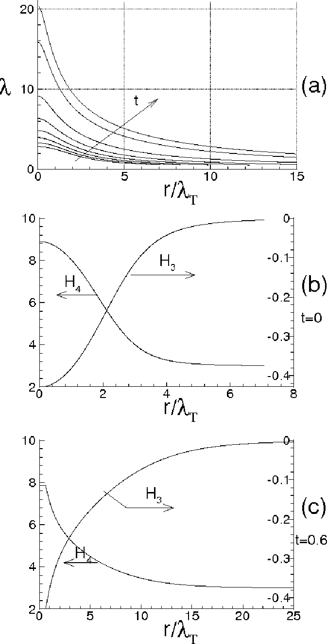
For the same simulation, Fig. 6a shows the maximal finite scale Lyapunov exponent, calculated with Eq. (29), where $\lambda$ varies according to $f$. For $t=0$, the variations of $\lambda$ are the result of the adopted initial correlation function which is a gaussian, whereas as the time increases, the variations of $f$ determine sizable increments of $\lambda$ and of its slope in proximity of the origin. Then, for developed spectrum, since $f-1$ = O($r^{2/3}$), the maximal finite scale Lyapunov exponent behaves like $\lambda\approx r^{-2/3}$. Thus, the diffusivity coefficient associated to the relative motion between two fluid particles, defined as $D(r)\propto\lambda r^{2}$, here satisfies the famous Richardson scaling law $D(r)\approx r^{4/3}$[4].

In the diagrams of Figs. 6b and 6c, skewness and flatness of $\Delta u_{r}$ are shown in terms of $r$ for $\bar{t}$ = 0 and 0.6. The skewness, $H_{3}$ is first calculated with Eq. (31), then $H_{4}$ has been determined using Eq. (IV). At $\bar{t}=0$, $|H_{3}|$ starts from 3/7 at the origin with small slope, then decreases until to reach small values. $H_{4}$ also exhibits small derivatives near the origin, where $H_{4}\gg$ 3, thereafter it decreases more rapidly than $|H_{3}|$. At $\bar{t}=$0.6, the diagram importantly changes and exhibits different shapes. The Taylor scale and the corresponding Reynolds number are both changed, so that the variations of $H_{3}$ and $H_{4}$ are associated to smaller distances, whereas the flatness at the origin is slightly less than that at $t=0$. Nevertheless, these variations correspond to higher $r/\lambda_{T}$ than those for $t$ = 0, and also in this case, $H_{4}$ reaches the value of 3 more rapidly than $H_{3}$ tends to zero.

The PDFs of $\Delta u_{r}$ are calculated with Eqs. (IV) and (IV), and are shown in Fig. 7 in terms of the dimensionless abscissa

where, these distribution functions are normalized, in order that their standard deviations are equal to the unity. The figure represents the distribution functions of $s$ for several $r/\lambda_{T}$, at $\bar{t}$ = 0, 0.5 and 0.6, where the dotted curves represent the gaussian distribution functions. The calculation of $H_{3}(r)$ is first carried out with Eq. (31), then the function $\psi(r,R_{\lambda})$ is identified through Eq. (66), and finally the PDF is obtained with Eq. (IV). For $t$ = 0 (see Fig. 7a) and according to the evolutions of $H_{3}$ and $H_{4}$, the PDFs calculated at $r/\lambda_{T}=$ 0 and 1, are quite similar each other, whereas for $r/\lambda_{T}=$ 5, the PDF is almost a gaussian function. Toward the end of the simulation, (see Fig. 7b and c), the two PDFs calculated at $r/\lambda_{T}=$ 0 and 1, exhibit more sizable differences, whereas for $r/\lambda_{T}=$ 5, the PDF differs very much from a gaussian PDF. This is in line with the plots of $H_{3}(r)$ and $H_{4}(r)$ of Fig. 6.

Next, the spatial structure of $\Delta u_{r}$, given by Eq. (IV), is analyzed using the previous results of the simulation. According to the various works [19, 20, 21], $\Delta u_{r}$ behaves quite similarly to a multifractal system, where $\Delta u_{r}$ obeys to a law of the kind $\Delta u_{r}(r)\approx r^{q}$ where the exponent $q$ is a fluctuating function of space. This implies that the statistical moments of $\Delta u_{r}(r)$ are expressed through different scaling exponents $\zeta(P)$ whose values depend on the moment order $P$, i.e.

These scaling exponents are here identified through a best fitting procedure, in the intervals ($a_{P},a_{P}$ $+\lambda_{T}$), where the endpoints $a_{P}$ are unknown quantities which have to be determined. The location of these intervals depends on $P$ and varies with the time. The calculation of the endpoints $a_{P}$ and of $\zeta_{P}$ and $A_{P}$ is carried out through a minimum square method which for each moment order is applied to the following optimization problem

where $(\langle\Delta u_{r}^{P})\rangle$ are calculated with Eqs. (IV).
Figure 8 shows the comparison between the scaling exponents here obtained (continuous lines with solid symbols) and those of the Kolmogorov theories K41 [5] (dashed lines) and K62 [19] (dashdotted lines), and those given by She-Leveque [20] (dotted curves). At $t=$ 0, the values of $\zeta(P)$ are the result of the chosen initial condition. As the time increases, the correlation function changes causing variations in the statistical moments of $\Delta u_{r}(r)$. As result, $\zeta(P)$ gradually diminish and exhibit a variable slope which depends on the moment order $P$, until to reach the situation of Fig. 8b, where the simulation is just ended. The dimensionless moments of $\Delta u_{r}(r)$ are changed. The plot of $\zeta(P)$ shows that near the origin, $\zeta(P)\simeq P/3$, and that the values of $\zeta(P)$ seem to be in agreement with the those proposed by She-Leveque. More in detail, Table I reports these scaling exponents in terms of the moments order, calculated for $\bar{t}=0.63$. These values are the consequence of the spatial variations of the skewness, calculated using Eq. (31), and of the quadratic terms due to the inertia and pressure forces into the expression of the velocity difference, which make $\langle(\Delta u_{r})^{P}\rangle$ a quantity quite similar to a multifractal system.

Other simulations with different initial correlation functions and Reynolds numbers have been carried out, and all of them lead to analogous results, in the sense that, at the end of the simulations, the diverse quantities such as $Q(r)$, $C$ and $\zeta(P)$ are quite similar to those just calculated. For what concerns the effect of the Reynolds number, its increment determines a wider range of the wave-numbers where $E(\kappa)$ is comparable with the Kolmogorov law and a smaller dissipation energy rate in accordance to Eq. (84).

In order to study the evolution of the intermittency vs. the Reynolds number, Table II gives the first ten statistical moments of $F(\partial u_{r}/\partial r)$. These are calculated with Eqs. (IV) and (IV), for $R_{\lambda}$ = 10.12, 100 and 1000, and are shown in comparison with those of a gaussian distribution function. It is apparent that a constant nonzero skewness of the longitudinal velocity derivative, causes an intermittency which rises with $R_{\lambda}$ (see Eq. (IV)). More specifically, Fig. 9 shows the variations of $H_{4}(0)$ and $H_{6}(0)$ (continuous lines) in terms of $R_{\lambda}$, calculated with Eqs. (IV) and (IV), with $H_{3}(0)=-3/7$. These moments are rising functions of $R_{\lambda}$ for 10 $\lesssim R_{\lambda}\lesssim$ 700, whereas for higher $R_{\lambda}$ these tend to the saturation and such behavior also happens for the other absolute moments. According to Eq. (IV), in the interval 10 $\lesssim R_{\lambda}\lesssim$ 70, $H_{4}$ and $H_{6}$ result to be about proportional to $R_{\lambda}^{0.34}$ and $R_{\lambda}^{0.78}$, respectively, and the intermittency increases with the Reynolds number until to $R_{\lambda}\approx$ 700, where it ceases to rise so quickly.

This behavior, represented by the continuous lines, depends on the fact that $\psi\approx\sqrt{R_{\lambda}}$, and results to be in very good agreement with the data of Pullin and Saffman [22], for 10 $\lesssim R_{\lambda}\lesssim$ 100.

Figure 9 can be compared with the data collected by Sreenivasan and Antonia [15], which are here reported into Fig. 10. These latter are referred to several measurements and simulations obtained in different situations which can be very far from the isotropy and homogeneity conditions. Nevertheless a comparison between the present results and those of Ref. [15] is an opportunity to state if the two data exhibit elements in common. According to Ref. [15], the flatness monotonically rises with $R_{\lambda}$ with a rising rate which agrees with Eq. (IV) for $10\lesssim R_{\lambda}\lesssim 60$ (dashed line, Fig. 9), whereas the skewness seems to exhibit minor variations. Thereafter, $H_{4}$ continues to rise with about the same rate, without the saturation observed in Fig. 9. The weaker intermittency calculated with the present analysis arise from the isotropy which makes the velocity fluctuation a gaussian random variable, while, as seen in sec. IV, without the isotropy condition, the flatness of velocity and of velocity difference can be much greater than that of the isotropic case.

Again, the obtained results are compared with the data of Tabeling et al [13, 14], where, in an experiment using low temperature helium gas between two counter-rotating cylinders (closed cell), the authors measure the PDF of $\partial u_{r}/\partial r$ and its moments. Also in this case the flow can be quite far from to the isotropy condition. In fact, these experiments pertain wall-bounded flows, where the walls could importantly influence the fluid velocity in proximity of the probe. The authors found that the higher moments than the third order, first increase with $R_{\lambda}$ until to $R_{\lambda}\approx$ 700, then exhibit a lightly non-monotonic evolution with respect to $R_{\lambda}$, and finally cease their variations denoting a transition behavior (See Fig. 11). As far as the skewness is concerned, the authors observe small percentage variations. Although the isotropy does not describe the non-monotonic evolution near $R_{\lambda}=$ 700, the results obtained with Eq. (IV) can be considered comparable with those of Refs. [13, 14], resulting also in this case, that the proposed analysis gives a weaker intermittency with respect to Refs. [13, 14].

The normalized PDFs of $\partial u_{r}/\partial r$ are calculated with Eqs. (IV) and (IV), and are shown in Fig. 12 in terms of the variable $s$, which is defined as

Figure 12a shows the diagrams for $R_{\lambda}=$ 15, 30 and 60, where the PDFs vary in such a way that $H_{3}(0)=-3/7$.
As well as in Ref. [14], Figs. 4b and 4c give the PDF for $R_{\lambda}$ = 255, 416, 514, 1035 and 1553, where these last Reynolds numbers are calculated through the Kolmogorov function given in Ref. [14], with $H_{3}(0)=-3/7$. In particular, Fig. 12c represents the enlarged region of Fig. 12b, where the tails of PDF are shown for $5<s<8$. According to Eq. (IV), the tails of the PDF rise in the interval 10 $\lesssim R_{\lambda}\lesssim$ 700, whereas at higher $R_{\lambda}$, smaller variations occur. Although the non-monotonic trend observed in Ref. [14], Fig. 12c shows that the values of the PDFs calculated with the proposed analysis, for $5<s<8$, exhibit the same order of magnitude of those obtained by Tabeling et al [14] which are here shown in Fig. 13.

Asymmetry and intermittency of the distribution functions are also represented through the integrand function of the $4^{th}$ order moment of PDF, which is $J_{4}(s)=s^{4}F(s)$. This function is shown in terms of $s$, in Fig. 14, for $R_{\lambda}$ = 15, 30 and 60.

References

- [1] Landau, L. D., Lifshitz, M, Fluid Mechanics. Pergamon London, England, 1959.
- [2] Ottino, J. M., Mixing, Chaotic Advection, and Turbulence., Annu. Rev. Fluid Mech. 22, 207–253, 1990.
- [3] Truesdell, C. A First Course in Rational Continuum Mechanics, Academic, New York, 1977.
- [4] Richardson, L. F, Atmospheric Diffusion shown on a distance–neighbour graph., Proc. Roy. Soc. London, A 110, 709, 1926.
- [5] Kolmogorov, A. N., Dissipation of Energy in Locally Isotropic Turbulence. Dokl. Akad. Nauk SSSR 32, 1, 19–21, 1941.
- [6] von Kármán, T. & Howarth, L., On the Statistical Theory of Isotropic Turbulence., Proc. Roy. Soc. A, 164, 14, 192, 1938.
- [7] Batchelor, G.K., The Theory of Homogeneous Turbulence. Cambridge University Press, Cambridge, 1953.
- [8] Guckenheimer, J., Holmes, P., Nonlinear Oscillations, Dynamical Systems, and Bifurcations of Vector Fields. Springer, 1990.
- [9] Lamb, H. Hydrodynamics, Dover Publications, 1945.
- [10] Christiansen, F., Rugh, H. H., Computing Lyapunov spectra with continuous Gram–Schmidt orthonormalization, Nonlinearity, Vol. 10, No. 5, pp. 1063–1072, 1997.
- [11] Ershov, S. V., Potapov, A. B., On the Concept of Stationary Lyapunov Basis., Physica D, 118, 167–198, 1998.
- [12] Prigogine, I., Time, Chaos and the Laws of Chaos. Ed. Progress, Moscow, 1994.
- [13] Tabeling, P., Zocchi, G., Belin, F., Maurer, J., Willaime, H., Probability density functions, skewness, and flatness in large Reynolds number turbulence, Phys. Rev. E 53, 1613, 1996.
- [14] Belin, F., Maurer, J. Willaime, H., Tabeling, P., Velocity Gradient Distributions in Fully Developed Turbulence: An Experimental Study, Physics of Fluid 9, no. 12, 3843–3850, 1997.
- [15] Sreenivasan, K. R., Antonia, R. A., The Phenomenology of Small–Scale Turbulence., Annu. Rev. Fluid Mech. 29, 435–472, 1997.
- [16] Lehmann, E.L., Elements of Large–sample Theory. Springer, 1999.
- [17] Madow, W. G., Limiting Distributions of Quadratic and Bilinear Forms., The Annals of Mathematical Statistics, Vol. 11, No. 2, (Jun. 1940), 125–146, 1940.
- [18] Hildebrand, F.B., Introduction to Numerical Analysis, Dover Publications, 1987.
- [19] Kolmogorov, A. N., Refinement of Previous Hypothesis Concerning the Local Structure of Turbulence in a Viscous Incompressible Fluid at High Reynolds Number, J. Fluid Mech. 12, 82–85, 1962.
- [20] She, Z.S. and Leveque, E., Universal scaling laws in fully developed turbulence, Phys. Rev. Lett. 72, 336, 1994.
- [21] Benzi, R., Biferale, L., Paladin, G., Vulpiani, A., Vergassola, M., Multifractality in the Statistics of the Velocity Gradients in Turbulence, Phys. Rev. Lett. 67, 2299, 1991.
- [22] Pullin, D., Saffman, P., On the Lundgren Townsend model of turbulent fine structure, Phys. Fluids, A 5, 1,126, 1993.
- [23] Feigenbaum, M. J., J. Stat. Phys. 19, 1978.
- [24] Ruelle, D. & Takens, F., Commun. Math Phys. 20, 167, 1971.
- [25] Pomeau, Y., Manneville, P., Commun Math. Phys. 74, 189, 1980.
- [26] Eckmann, J.P., Roads to turbulence in dissipative dynamical systems Rev. Mod. Phys. 53, 643–654, 1981.
- [27] Gollub, J.P., Swinney, H.L., Onset of Turbulence in a Rotating Fluid., Phys. Rev. Lett. 35, 927, 1975.
- [28] Giglio M., Musazzi S., Perini U., Transition to chaotic behavior via a reproducible sequence of period doubling bifurcations, Phys. Rev. Lett. 47, 243, 1981.
- [29] Maurer, J., Libchaber A., Rayleigh–Bénard Experiment in Liquid Helium: Frequency Locking and the onset of turbulence, Journal de Physique Letters 40, L419–L423, 1979.