跳到论文正文
W Papers独立论文阅读器 arXiv:0905.3506 论文正文 计算阅读时间 · 0%
引用这篇论文根据当前论文元数据生成,正式投稿前建议核对。


License: arXiv.org perpetual non-exclusive license
arXiv:0905.3506v3 [hep-ph] 21 Sep 2010

Chiral corrections to heavy quark-diquark symmetry predictions for doubly heavy baryon zero-recoil semileptonic decay

Jie Hu Email: hujie@ust.hk Affiliation: Department of Physics, Duke University, Durham, North Carolina 27708, USA Affiliation: Department of Chemistry, Hong Kong University of Science and Technology, Kowloon, Hong Kong
August 24, 2026
Abstract

This paper studies the leading chiral corrections to heavy quark-diquark symmetry predictions for doubly heavy baryon semileptonic decay form factors. We derive the coupling between heavy diquarks and weak current in the limit of heavy quark-diquark symmetry, and construct the chiral Lagrangian for doubly heavy baryons coupled to weak current. We evaluate chiral corrections to doubly heavy baryon zero-recoil semileptonic decay for both unquenched and partially quenched QCD. This theory is used to derive chiral extrapolation expressions for measurements of form factors of doubly heavy baryon zero-recoil semileptonic decay in lattice QCD simulations.

pacs
12.39.Fe, 12.39.Hg, 14.20.Lq

I Introduction

This work is stimulated by the recent SELEX experimental observation on states which have been tentatively interpreted as doubly charm baryons [1, 2, 3]. The masses and hyperfine splittings of the observed states are consistent with theoretical predictions from some quark models [4] and quenched lattice quantum chromodynamics (QCD)  [5, 6, 7]. However many other aspects are difficult to understand in the current theoretical framework, such as the missing weak decay signal of the higher state in the ground doublet. Model-independent predictions for doubly heavy baryon properties would be helpful. Chiral and heavy quark symmetries are useful approximate symmetries of QCD for predicting low-energy properties of hadrons containing a single heavy quark. Heavy quark-diquark symmetry relates the properties of heavy mesons with a single heavy quark (Q​q¯Q\bar{q}) to those of doubly heavy anti-baryons with two heavy anti-quarks (Q¯​Q¯​q¯\bar{Q}\bar{Q}\bar{q}). The heavy quark-diquark symmetry prediction for the doubly charm baryon hyperfine splitting [8, 9, 5, 4] is within 25∼30%25\sim 30\% of the quenched lattice QCD calculation. More observables are needed to see whether the heavy quark-diquark symmetry is applicable to charm and bottom. Semileptonic decay of doubly charm baryons was studied previously using model dependent method [10] and recently by the heavy quark spin symmetry [11]. However the latter provided only tree level predictions of doubly heavy baryon semileptonic decay matrices.

In this paper we will study the chiral corrections to heavy quark-diquark symmetry predictions for the form factors of zero-recoil doubly heavy baryon semileptonic decay, and further arrive at the results for both unquenched and partially quenched QCD.

We use the techniques in non-relativistic quantum chromodynamics (NRQCD) to derive the coupling between heavy diquarks and weak current. Savage and Wise [12] wrote an effective Lagrangian for heavy quarks and diquarks using heavy quark effective theory (HQET) [13] and calculated the doubly heavy baryon hyperfine splittings. HQET is formulated as an expansion in the heavy quark mass scaled ΛQ​C​D/mQ\Lambda_{QCD}/m_{Q}. Hadrons with two or more heavy quarks, such as quarkonia or doubly heavy baryons, are characterized by the additional scales mQ​vm_{Q}v and mQ​v2m_{Q}v^{2}, where vv is the typical velocity of the heavy quark within the bound state. The dynamics of hadrons with two or more heavy quarks follows NRQCD [14, 15, 16]. Within this framework the effective Lagrangian for heavy diquark have been derived recently [8, 9], which corrected the hyperfine splitting predictions of Ref. 12 by a factor of 22.

For studying the low-energy dynamics of hadrons containing diquark, it is useful to build an effective theory which incorporates the relevant symmetries of QCD. Heavy hadron chiral perturbation theory (HHχ\chiPT) [17, 18, 19] has heavy hadrons, Goldstone bosons, and photons as its elementary degrees of freedom and incorporates chiral and heavy quark symmetries. Hu and Mehen [20] derived an effective Lagrangian for doubly heavy baryons incorporating heavy quark-diquark symmetry and used this theory to study strong and electromagnetic interactions of doubly heavy baryons in low-energy regime. Here we will apply HHχ\chiPT to evaluate chiral corrections to semileptonic decay at zero-recoil.

Moreover, we will extend the chiral Lagrangian with heavy quark-diquark symmetry to include lattice effects of partial quenching. We derive expressions for the chiral extrapolation of zero-recoil semileptonic decay of double heavy baryons in lattice calculation. Lattice calculations of decay matrix elements of heavy mesons and doubly heavy baryons can help determine the reliability of heavy quark-diquark symmetry for charm and bottom hadrons. High-precision lattice calculation of semileptonic decay form factors of heavy mesons is a long term project of several collaborations, such as HPQCD and MILC. Lattice QCD simulations start with unphysical sea quark masses which need to be extrapolated to physical values. Chiral Lagrangians in quenched [21] and partially quenched [22, 23] theory are useful for the chiral extrapolations of the lattice simulation data.

The rest of the paper is organized as follows. In Sec. II, we use NRQCD to derive the coupling between heavy diquarks and weak current consistent with heavy quark-diquark symmetry. In Sec. III, we construct the chiral Lagrangian for doubly heavy baryons coupled to weak current and calculate the doubly heavy baryon zero-recoil semileptonic decay matrix elements. We evaluate the chiral corrections to the decay form factors using χ\chiPT. In the heavy quark-diquark limit the corrections vanish. In Sec. IV, we extend the chiral Lagrangian with heavy quark-diquark symmetry to partially quenched theory and derive form factor formulism for the lattice QCD chiral extrapolation of doubly heavy baryon zero-recoil semileptonic decay, via partial quenching versus unquenching. Summary is given in Sec. V. Some useful formulations are collected in Appendix.

II Coupling between Heavy Diquarks and Weak Current from vvNRQCD

NRQCD is the nonrelativistic effective theory for the dynamics of heavy quarks. In NRQCD the important scales are among the four quantities: the heavy quark mass mQm_{Q}, the typical momentum mQ​vm_{Q}v of heavy quarks within bound state, the typical kinetic energy mQ​v2m_{Q}v^{2} of heavy quarks, and ΛQ​C​D\Lambda_{QCD}. The total momentum of heavy quark field is taken to be the sum of the labeling momentum 𝐩(∼mQ​v)\mathbf{p}(\sim m_{Q}v) and the residual momentum 𝐤(∼mQ​v2)\mathbf{k}(\sim m_{Q}v^{2}). In vvNRQCD [9], which has a consistent vv expansion, the Lagrangian for Q¯​Q¯\bar{Q}\bar{Q} (Q¯=b¯,c¯\bar{Q}=\bar{b},\bar{c}) of the leading order reads

ℒ\displaystyle\mathcal{L} =−14​Fμ​ν​Fμ​ν\displaystyle=-\frac{1}{4}F^{\mu\nu}F_{\mu\nu}
+∑f=b,c∑𝐩χ𝐩f†(iD0−(𝐩−i​𝐃)22​mQf+gs2​mQf𝝈⋅𝐁)χ𝐩f\displaystyle\quad+\sum_{f=b,c}\sum_{\mathbf{p}}\chi_{\mathbf{p}}^{f{\dagger}}\Big(iD_{0}-\frac{(\mathbf{p}-i\mathbf{D})^{2}}{2m_{Q_{f}}}+\frac{g_{s}}{2m_{Q_{f}}}{\bm{\sigma}}\cdot\mathbf{B}\Big)\chi_{\mathbf{p}}^{f}
−12∑f=b,c∑𝐩,𝐪gs2(𝐩−𝐪)2χ𝐪f†T¯Aχ𝐩fχ−𝐪f†T¯Aχ−𝐩f\displaystyle\quad-\frac{1}{2}\sum_{f=b,c}\sum_{\mathbf{p,q}}\frac{g_{s}^{2}}{(\mathbf{p}-\mathbf{q})^{2}}\chi_{\mathbf{q}}^{f{\dagger}}\bar{T}^{A}\chi_{\mathbf{p}}^{f}\chi_{-\mathbf{q}}^{f{\dagger}}\bar{T}^{A}\chi_{-\mathbf{p}}^{f}
−∑𝐩,𝐪gs2(𝐩−𝐪)2χ𝐪b†T¯Aχ𝐩bχ−𝐪c†T¯Aχ−𝐩c+⋯.\displaystyle\quad-\sum_{\mathbf{p,q}}\frac{g_{s}^{2}}{(\mathbf{p}-\mathbf{q})^{2}}\chi_{\mathbf{q}}^{b{\dagger}}\bar{T}^{A}\chi_{\mathbf{p}}^{b}\chi_{-\mathbf{q}}^{c{\dagger}}\bar{T}^{A}\chi_{-\mathbf{p}}^{c}+\cdots. (1)

Here χ𝐩f\chi_{\mathbf{p}}^{f} is a nonrelativistic anti-quark field which annihilates an anti-quark of flavor ff, T¯A\bar{T}^{A} is S​U​(3)SU(3) color generator for 3¯\bar{3} representation, 𝐁\mathbf{B} is chromomagnetic field, and D0D_{0} and 𝐃\mathbf{D} are the time and spatial components of the gauge covariant derivative, respectively. The kinetic energy D0D_{0} and momentum 𝐩\mathbf{p} of heavy anti-quark field are of O⁡(mQ​v2)O(m_{Q}v^{2}) and O⁡(mQ​v)O(m_{Q}v), respectively.

In order to derive an effective Lagrangian for diquark we follow the methods of Ref. 9. We use the spin and color Fierz identities

,
δα​δ​δβ​γ\displaystyle\delta_{\alpha\delta}\delta_{\beta\gamma} =−12​(σi​ϵ)α​β​(ϵ​σi)γ​δ+12​ϵα​β​ϵγ​δT,\displaystyle=-\frac{1}{2}(\sigma^{i}\epsilon)_{\alpha\beta}(\epsilon\sigma^{i})_{\gamma\delta}+\frac{1}{2}\epsilon_{\alpha\beta}\epsilon^{T}_{\gamma\delta}\,, (2a)
T¯i​lA​T¯j​kA\displaystyle\bar{T}^{A}_{il}\bar{T}^{A}_{jk} =23​∑m12​ϵm​i​j​ϵm​k​l+13​∑(m​n)di​j(m​n)​dk​l(m​n),\displaystyle=\frac{2}{3}\sum_{m}\frac{1}{2}\epsilon_{mij}\epsilon_{mkl}+\frac{1}{3}\sum_{(mn)}d^{(mn)}_{ij}d^{(mn)}_{kl}, (2b)

respectively, to decompose the anti-quark bilinear such as χ𝐩f​χ−𝐩f\chi_{\mathbf{p}}^{f}\chi_{\mathbf{-p}}^{f} into operators with spin 00 and spin 11, and to project the potential onto the 𝟑\mathbf{3} and 𝟔¯\bar{\mathbf{6}} channels. In Eq. (2) the Greek subindexes denote spins and the Roman subindexes denote colors. σi\sigma^{i} are Pauli matrices, ϵ=i​σ2\epsilon=i\sigma^{2}, and di​j(m​n)d^{(mn)}_{ij} are elements of symmetric matrices in color space defined by

di​j(m​n)={(δm​i​δn​j+δn​i​δm​j)/2,m≠nδm​i​δn​j,m=n.d^{(mn)}_{ij}=\left\{\begin{array}[]{cc}(\delta_{mi}\delta_{nj}+\delta_{ni}\delta_{mj})/\sqrt{2},&m\neq n\\ \delta_{mi}\delta_{nj},&m=n\end{array}\right.. (3)

The diquark states, b¯​b¯\bar{b}\bar{b} and c¯​c¯\bar{c}\bar{c}, must be only in (𝟑)C​(𝟑)S(\mathbf{3})_{C}(\mathbf{3})_{S} or (𝟔¯)C​(𝟏)S(\bar{\mathbf{6}})_{C}(\mathbf{1})_{S} by the Pauli principle, while b¯​c¯\bar{b}\bar{c} can also be in (𝟑)C​(𝟏)S(\mathbf{3})_{C}(\mathbf{1})_{S} or (𝟔¯)C​(𝟑)S(\bar{\mathbf{6}})_{C}(\mathbf{3})_{S}. By fourier transforming gs2(𝐩−𝐪)2=∫d3​𝐫​gs24​π​r​ei⁡(𝐩−𝐪)⋅𝐫\frac{g_{s}^{2}}{(\mathbf{p}-\mathbf{q})^{2}}=\int d^{3}\mathbf{r}\frac{g_{s}^{2}}{4\pi r}e^{i(\mathbf{p}-\mathbf{q})\cdot\mathbf{r}}, Eq. (1) leads to

ℒ\displaystyle\mathcal{L} =−14Fμ​νFμ​ν+∑f=b,c∑𝐩χ𝐩f†(iD0−(𝐩−i​𝐃)22​mQf+gs2​mQf𝝈⋅𝐁)χ𝐩f\displaystyle=-\frac{1}{4}F^{\mu\nu}F_{\mu\nu}+\sum_{f=b,c}\sum_{\mathbf{p}}\chi_{\mathbf{p}}^{f{\dagger}}\Big(iD_{0}-\frac{(\mathbf{p}-i\mathbf{D})^{2}}{2m_{Q_{f}}}+\frac{g_{s}}{2m_{Q_{f}}}{\bm{{\sigma}}}\cdot\mathbf{B}\Big)\chi_{\mathbf{p}}^{f}
−12∑f=b,c∫d3𝐫V(3)(r)(∑𝐪e−i𝐪⋅𝐫ϵm​i​j2(χ𝐪f†)i𝝈ϵ(χ−𝐪f†)j)⋅(∑𝐩ei​𝐩⋅𝐫ϵm​k​l2(χ−𝐩f)kϵ𝝈(χ𝐩f)l)\displaystyle\quad-\frac{1}{2}\sum_{f=b,c}\int d^{3}\mathbf{r}V^{(3)}(r)\Big(\sum_{\mathbf{q}}e^{-i\mathbf{q}\cdot\mathbf{r}}\frac{\epsilon_{mij}}{2}(\chi_{\mathbf{q}}^{f{\dagger}})_{i}{\bm{{\sigma}}}\epsilon(\chi_{\mathbf{-q}}^{f{\dagger}})_{j}\Big)\cdot\Big(\sum_{\mathbf{p}}e^{i\mathbf{p}\cdot\mathbf{r}}\frac{\epsilon_{mkl}}{2}(\chi_{\mathbf{-p}}^{f})_{k}\epsilon{\bm{{\sigma}}}(\chi_{\mathbf{p}}^{f})_{l}\Big)
−∫d3𝐫V(3)(r)(∑𝐪e−i𝐪⋅𝐫ϵm​i​j2(χ𝐪b†)i𝝈ϵ(χ−𝐪c†)j)⋅(∑𝐩ei​𝐩⋅𝐫ϵm​k​l2(χ−𝐩c)kϵ𝝈(χ𝐩b)l)\displaystyle\quad-\int d^{3}\mathbf{r}V^{(3)}(r)\Big(\sum_{\mathbf{q}}e^{-i\mathbf{q}\cdot\mathbf{r}}\frac{\epsilon_{mij}}{2}(\chi_{\mathbf{q}}^{b{\dagger}})_{i}{\bm{{\sigma}}}\epsilon(\chi_{\mathbf{-q}}^{c{\dagger}})_{j}\Big)\cdot\Big(\sum_{\mathbf{p}}e^{i\mathbf{p}\cdot\mathbf{r}}\frac{\epsilon_{mkl}}{2}(\chi_{\mathbf{-p}}^{c})_{k}\epsilon{\bm{{\sigma}}}(\chi_{\mathbf{p}}^{b})_{l}\Big)
−∫d3𝐫V(3)(r)(−∑𝐪e−i𝐪⋅𝐫ϵm​i​j2(χ𝐪b†)iϵ(χ−𝐪c†)j)(∑𝐩ei​𝐩⋅𝐫ϵm​k​l2(χ−𝐩c)kϵT(χ𝐩b)l)+∫d3𝐫V(6¯)(r)[⋯],\displaystyle\quad-\int d^{3}\mathbf{r}V^{(3)}(r)\Big(-\sum_{\mathbf{q}}e^{-i\mathbf{q}\cdot\mathbf{r}}\frac{\epsilon_{mij}}{2}(\chi_{\mathbf{q}}^{b{\dagger}})_{i}\epsilon(\chi_{\mathbf{-q}}^{c{\dagger}})_{j}\Big)\Big(\sum_{\mathbf{p}}e^{i\mathbf{p}\cdot\mathbf{r}}\frac{\epsilon_{mkl}}{2}(\chi_{\mathbf{-p}}^{c})_{k}\epsilon^{T}(\chi_{\mathbf{p}}^{b})_{l}\Big)+\int d^{3}\mathbf{r}V^{(\bar{6})}(r)[\cdots], (4)

where V(3)​(r)=−23​αsrV^{(3)}(r)=-\frac{2}{3}\frac{\alpha_{s}}{r}. The last term with V(6¯)​(r)=13​αsrV^{(\bar{6})}(r)=\frac{1}{3}\frac{\alpha_{s}}{r} is irrelevant to color neutral doubly heavy baryon and is therefore dropped out hereafter. The first term is the gauge boson field. The second term includes the kinetic operators for the anti-quark fields and the leading spin symmetry breaking interactions which generate hyperfine splittings. The other terms are the quartic terms with diquark fields.

The diquark fields for c¯​c¯\bar{c}\bar{c} and b¯​b¯\bar{b}\bar{b} can be introduced using the Hubbard-Strantonovich transformation as Ref. 9. In addition, we introduce diquark field of different flavor b¯​c¯\bar{b}\bar{c} to get the interaction for doubly heavy baryon semileptonic decay. We add to the Lagrangian in Eq. (4) the following identity of Δ​ℒ=0\Delta\mathcal{L}=0:

Δ​ℒ\displaystyle\Delta\mathcal{L} =12∑f=b,c∫d3𝐫V(3)(r)(𝐓𝐫m†−∑𝐪e−i𝐪⋅𝐫ϵm​i​j2(χ𝐪f†)i𝝈ϵ(χ−𝐪f†)j)⋅(𝐓𝐫m−∑𝐩ei​𝐩⋅𝐫ϵm​k​l2(χ−𝐩f)kϵ𝝈(χ𝐩f)l)\displaystyle=\frac{1}{2}\sum_{f=b,c}\int d^{3}\mathbf{r}V^{(3)}(r)\Big(\!\mathbf{T}^{m{\dagger}}_{\mathbf{r}}\!-\!\sum_{\mathbf{q}}\!e^{-i\mathbf{q}\cdot\mathbf{r}}\frac{\epsilon_{mij}}{2}(\chi_{\mathbf{q}}^{f{\dagger}})_{i}{\bm{{\sigma}}}\epsilon(\chi_{\mathbf{-q}}^{f{\dagger}})_{j}\!\Big)\!\cdot\!\Big(\!\mathbf{T}^{m}_{\mathbf{r}}\!-\!\sum_{\mathbf{p}}\!e^{i\mathbf{p}\cdot\mathbf{r}}\frac{\epsilon_{mkl}}{2}(\chi_{\mathbf{-p}}^{f})_{k}\epsilon{\bm{{\sigma}}}(\chi_{\mathbf{p}}^{f})_{l}\!\Big)\!
+∫d3𝐫V(3)(r)(𝐓~𝐫m†−∑𝐪e−i𝐪⋅𝐫ϵm​i​j2(χ𝐪b†)i𝝈ϵ(χ−𝐪c†)j)⋅(𝐓~𝐫m−∑𝐩ei​𝐩⋅𝐫ϵm​k​l2(χ−𝐩c)kϵ𝝈(χ𝐩b)l)\displaystyle\quad+\!\int\!d^{3}\mathbf{r}V^{(3)}(r)\!\Big(\!\tilde{\mathbf{T}}^{m{\dagger}}_{\mathbf{r}}\!-\!\sum_{\mathbf{q}}\!e^{-i\mathbf{q}\cdot\mathbf{r}}\frac{\epsilon_{mij}}{2}(\chi_{\mathbf{q}}^{b{\dagger}})_{i}{\bm{{\sigma}}}\epsilon(\chi_{\mathbf{-q}}^{c{\dagger}})_{j}\!\Big)\!\cdot\!\Big(\!\tilde{\mathbf{T}}^{m}_{\mathbf{r}}\!-\!\sum_{\mathbf{p}}\!e^{i\mathbf{p}\cdot\mathbf{r}}\frac{\epsilon_{mkl}}{2}(\chi_{\mathbf{-p}}^{c})_{k}\epsilon{\bm{{\sigma}}}(\chi_{\mathbf{p}}^{b})_{l}\!\Big)\!
+∫d3𝐫V(3)(r)(T𝐫′m†+∑𝐪e−i𝐪⋅𝐫ϵm​i​j2(χ𝐪b†)iϵ(χ−𝐪c†)j)(T𝐫′m−∑𝐩ei​𝐩⋅𝐫ϵm​k​l2(χ−𝐩c)kϵT(χ𝐩b)l),\displaystyle\quad+\!\int\!d^{3}\mathbf{r}V^{(3)}(r)\!\Big(\!T^{\prime m{\dagger}}_{\mathbf{r}}+\!\sum_{\mathbf{q}}e^{-i\mathbf{q}\cdot\mathbf{r}}\frac{\epsilon_{mij}}{2}(\chi_{\mathbf{q}}^{b{\dagger}})_{i}\epsilon(\chi_{\mathbf{-q}}^{c{\dagger}})_{j}\!\Big)\!\Big(\!T^{\prime m}_{\mathbf{r}}-\!\sum_{\mathbf{p}}e^{i\mathbf{p}\cdot\mathbf{r}}\frac{\epsilon_{mkl}}{2}(\chi_{\mathbf{-p}}^{c})_{k}\epsilon^{T}(\chi_{\mathbf{p}}^{b})_{l}\!\Big)\!, (5)

where m=1,2,3m=1,2,3 is the color index. 𝐓m=∑𝐩ei​𝐩⋅𝐫​ϵm​k​l2​(χ−𝐩f)k​ϵ​𝝈​(χ𝐩f)l\mathbf{T}^{m}=\sum_{\mathbf{p}}e^{i\mathbf{p}\cdot\mathbf{r}}\frac{\epsilon_{mkl}}{2}(\chi_{\mathbf{-p}}^{f})_{k}\epsilon{\bm{{\sigma}}}(\chi_{\mathbf{p}}^{f})_{l}, 𝐓~m=∑𝐩ei​𝐩⋅𝐫​ϵm​k​l2​(χ−𝐩c)k​ϵ​𝝈​(χ𝐩b)l\tilde{\mathbf{T}}^{m}=\sum_{\mathbf{p}}e^{i\mathbf{p}\cdot\mathbf{r}}\frac{\epsilon_{mkl}}{2}(\chi_{\mathbf{-p}}^{c})_{k}\epsilon{\bm{{\sigma}}}(\chi_{\mathbf{p}}^{b})_{l}, and T′m=∑𝐩ei​𝐩⋅𝐫​ϵm​k​l2​(χ−𝐩c)k​ϵT​(χ𝐩b)lT^{\prime m}=\sum_{\mathbf{p}}e^{i\mathbf{p}\cdot\mathbf{r}}\frac{\epsilon_{mkl}}{2}(\chi_{\mathbf{-p}}^{c})_{k}\epsilon^{T}(\chi_{\mathbf{p}}^{b})_{l} annihilate a spin-11 f¯​f¯\bar{f}\bar{f} field, a spin-11 b¯​c¯\bar{b}\bar{c} field, and a spin-00 b¯​c¯\bar{b}\bar{c} field, respectively. The quartic terms of anti-quark fields in the combination of Eq. (4) and Eq. (5) are cancelled, resulting in

ℒ\displaystyle\mathcal{L} =12∑f=b,c∫d3𝐫V(3)(r)(𝐓𝐫m†𝐓𝐫m−𝐓𝐫m†∑𝐩ei​𝐩⋅𝐫ϵm​k​l2(χ−𝐩f)kϵ𝝈(χ𝐩f)l−𝐓𝐫m∑𝐪e−i𝐪⋅𝐫ϵm​i​j2(χ𝐪f†)i𝝈ϵ(χ−𝐪f†)j)\displaystyle=\frac{1}{2}\sum_{f=b,c}\int d^{3}\mathbf{r}\,V^{(3)}(r)\Big(\mathbf{T}^{m{\dagger}}_{\mathbf{r}}\mathbf{T}^{m}_{\mathbf{r}}-\mathbf{T}^{m{\dagger}}_{\mathbf{r}}\sum_{\mathbf{p}}e^{i\mathbf{p}\cdot\mathbf{r}}\frac{\epsilon_{mkl}}{2}(\chi_{\mathbf{-p}}^{f})_{k}\epsilon\mbox{\boldmath$\sigma$}(\chi_{\mathbf{p}}^{f})_{l}-\mathbf{T}^{m}_{\mathbf{r}}\sum_{\mathbf{q}}e^{-i\mathbf{q}\cdot\mathbf{r}}\frac{\epsilon_{mij}}{2}(\chi_{\mathbf{q}}^{f{\dagger}})_{i}\mbox{\boldmath$\sigma$}\epsilon(\chi_{\mathbf{-q}}^{f{\dagger}})_{j}\Big)
+∫d3𝐫V(3)(r)(𝐓~𝐫m†𝐓~𝐫m−𝐓~𝐫m†∑𝐩ei​𝐩⋅𝐫ϵm​k​l2(χ−𝐩c)kϵ𝝈(χ𝐩b)l−𝐓~𝐫m∑𝐪e−i𝐪⋅𝐫ϵm​i​j2(χ𝐪b†)i𝝈ϵ(χ−𝐪c†)j)\displaystyle\quad+\int d^{3}\mathbf{r}V^{(3)}(r)\Big(\tilde{\mathbf{T}}^{m{\dagger}}_{\mathbf{r}}\tilde{\mathbf{T}}^{m}_{\mathbf{r}}-\tilde{\mathbf{T}}^{m{\dagger}}_{\mathbf{r}}\sum_{\mathbf{p}}e^{i\mathbf{p}\cdot\mathbf{r}}\frac{\epsilon_{mkl}}{2}(\chi_{\mathbf{-p}}^{c})_{k}\epsilon\mbox{\boldmath$\sigma$}(\chi_{\mathbf{p}}^{b})_{l}-\tilde{\mathbf{T}}^{m}_{\mathbf{r}}\sum_{\mathbf{q}}e^{-i\mathbf{q}\cdot\mathbf{r}}\frac{\epsilon_{mij}}{2}(\chi_{\mathbf{q}}^{b{\dagger}})_{i}\mbox{\boldmath$\sigma$}\epsilon(\chi_{\mathbf{-q}}^{c{\dagger}})_{j}\!\Big)
+∫d3𝐫V(3)(r)(T𝐫′m†T𝐫′m−T𝐫′m†∑𝐩ei​𝐩⋅𝐫ϵm​k​l2(χ−𝐩c)kϵT(χ𝐩b)l+T𝐫′m∑𝐪e−i𝐪⋅𝐫ϵm​i​j2(χ𝐪b†)iϵ(χ−𝐪c†)j).\displaystyle\quad+\int d^{3}\mathbf{r}V^{(3)}(r)\Big(T^{\prime m{\dagger}}_{\mathbf{r}}T^{\prime m}_{\mathbf{r}}-T^{\prime m{\dagger}}_{\mathbf{r}}\sum_{\mathbf{p}}e^{i\mathbf{p}\cdot\mathbf{r}}\frac{\epsilon_{mkl}}{2}(\chi_{\mathbf{-p}}^{c})_{k}\epsilon^{T}(\chi_{\mathbf{p}}^{b})_{l}+T^{\prime m}_{\mathbf{r}}\sum_{\mathbf{q}}e^{-i\mathbf{q}\cdot\mathbf{r}}\frac{\epsilon_{mij}}{2}(\chi_{\mathbf{q}}^{b{\dagger}})_{i}\epsilon(\chi_{\mathbf{-q}}^{c{\dagger}})_{j}\Big). (6)

Integrating out the fields 𝐓𝐫m\mathbf{T}^{m}_{\mathbf{r}}, 𝐓~𝐫m\tilde{\mathbf{T}}^{m}_{\mathbf{r}} and T𝐫′mT^{\prime m}_{\mathbf{r}} in Eq. (6) recovers the original NRQCD Lagrangian; integrating out the anti-quark fields χ𝐩b\chi^{b}_{\mathbf{p}} and χ−𝐩c\chi^{c}_{-\mathbf{p}} yields an effective action for the diquark fields 𝐓𝐫m\mathbf{T}^{m}_{\mathbf{r}}, 𝐓~𝐫m\tilde{\mathbf{T}}^{m}_{\mathbf{r}} and T𝐫′mT^{\prime m}_{\mathbf{r}}. The kinetic terms of b¯​c¯\bar{b}\bar{c} fields are the same as those of c¯​c¯\bar{c}\bar{c} fields in Ref. 9, with the proper diquark reduced mass μQ=(mb+mc)/(mb​mc)\mu_{Q}=(m_{b}+m_{c})/(m_{b}m_{c}). The Feynman rules for the coupling between the diquark field and the pair of anti-quarks in Eq. (6) are shown in Fig. 1.

Refer to caption
Figure 1: Feynman rules for the coupling between the diquark (𝐓𝐫m,𝐓~𝐫m\mathbf{T}_{\mathbf{r}}^{m},\tilde{\mathbf{T}}_{\mathbf{r}}^{m} or T𝐫′mT^{\prime m}_{\mathbf{r}}) and anti-quarks. The Greek indexes denote spins and the Roman indexes refer to colors.
Refer to caption
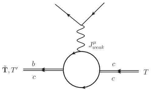
Figure 2: One loop diagram contributing to the coupling between composite anti-diquark fields and weak current.

Flavor changing weak current is given by JQ​C​Dμ=c¯​γμ​(1−γ5)​bJ^{\mu}_{QCD}=\bar{c}\gamma^{\mu}(1-\gamma_{5})b and is rewritten as JN​Rμ=χc†(δμ​0−δμ​iσi)χbJ^{\mu}_{NR}=\chi^{c{\dagger}}(\delta_{\mu 0}-\delta_{\mu i}\sigma^{i})\chi^{b} by mapping onto NRQCD to the lowest order. The coupling between anti-diquarks and weak current is to be evaluated by the lowest order diagram as in Fig. 2 and the resulting Lagrangian for weak interactions is

ℒweak\displaystyle\mathcal{L}_{\rm weak} =JQ¯​Q¯μ​(Jweak)μ,\displaystyle=J^{\mu}_{\bar{Q}\bar{Q}}(J_{\rm weak})_{\mu},
=−∫d3𝐫[δμ​0𝐓𝐫i†⋅𝐓~𝐫i+iδμ​n(𝐓𝐫i†×𝐓~𝐫i)n\displaystyle=-\int d^{3}\mathbf{r}\big[\delta_{\mu 0}\mathbf{T}^{i{\dagger}}_{\mathbf{r}}\cdot\tilde{\mathbf{T}}^{i}_{\mathbf{r}}+i\delta_{\mu n}(\mathbf{T}^{i{\dagger}}_{\mathbf{r}}\times\tilde{\mathbf{T}}^{i}_{\mathbf{r}})^{n}
+δμ​n(T𝐫i†)nT𝐫′i](Jweak)μ,\displaystyle\quad+\delta_{\mu n}(T^{i{\dagger}}_{\mathbf{r}})^{n}T^{\prime i}_{\mathbf{r}}\big](J_{\rm weak})_{\mu},
≈−η[δμ​0𝐓i†⋅𝐓~i+iδμ​n(𝐓i†×𝐓~i)n\displaystyle\approx-\eta\big[\delta_{\mu 0}\mathbf{T}^{i{\dagger}}\cdot\tilde{\mathbf{T}}^{i}+i\delta_{\mu n}(\mathbf{T}^{i{\dagger}}\times\tilde{\mathbf{T}}^{i})^{n}
+δμ​n(Ti†)nT′i](Jweak)μ,\displaystyle\quad+\delta_{\mu n}(T^{i{\dagger}})^{n}T^{\prime i}\big](J_{\rm weak})_{\mu}, (7)

where (Jweak)μ(J_{\rm weak})_{\mu} is the weak current and JQ¯​Q¯μJ^{\mu}_{\bar{Q}\bar{Q}} is the diquark current. In the last identity we expanded the diquark fields to the lowest order and wrote the Lagrangian in terms of local current. The factor η\eta can be interpreted as the spatial wavefunction overlap of the ground state initial diquark with the ground state final diquark system, which is not predicted by symmetry, i.e. η=∫d3​𝐫​ϕc¯​c¯∗​(𝐫)​ϕb¯​c¯​(𝐫)\eta=\int d^{3}\mathbf{r}\phi^{\ast}_{\bar{c}\bar{c}}(\mathbf{r})\phi_{\bar{b}\bar{c}}(\mathbf{r}).

III Doubly Heavy Baryon Semileptonic Decay

In the heavy quark limit, the ground states of the spin-00 heavy meson PP and the spin-11 heavy meson 𝐏∗\mathbf{P}^{\ast} are degenerate, and therefore combined into a single field,

Ha,α​β=(𝐏a∗⋅𝝈)α​β+Pa,α​β,\displaystyle H_{a,{\alpha}{\beta}}=(\mathbf{P}^{\ast}_{a}\cdot{\bm{\sigma}})_{{\alpha}{\beta}}+P_{a,{\alpha}{\beta}}\,, (8)

where aa is S​U​(3)SU(3) flavor anti-fundamental index and 𝝈{\bm{\sigma}} is the vector of Pauli matrices. Similarly in the heavy quark limit, the doubly heavy anti-baryon ground state doublet Ti​βT_{i\beta} consists of a spin-12\frac{1}{2} doubly heavy anti-baryon Ξa,γ\Xi_{a,\gamma} and a spin-32\frac{3}{2} doubly heavy anti-baryon Ξa,i​β∗\Xi^{\ast}_{a,i\beta} as

Ta,i​β=2​(Ξa,i​β∗+13​Ξa,γ​σγ​βi).\displaystyle T_{a,i\beta}=\sqrt{2}\Big(\Xi^{\ast}_{a,i\beta}+\frac{1}{\sqrt{3}}\Xi_{a,\gamma}\,\sigma^{i}_{\gamma\beta}\Big)\,. (9)

Hereafter TT denotes the doubly heavy anti-baryon field rather than the anti-diquark field in the previous section. In Eq. (9) the index of diquark spin runs as i=1,2,3i=1,2,3 and that of light anti-quark spin as β=1,2\beta=1,2. The field Ξa,i​β∗\Xi^{\ast}_{a,i\beta} obeys the constraint Ξa,i​β∗​σβ​γi=0\Xi^{\ast}_{a,i\beta}\,\sigma^{i}_{\beta\gamma}=0. Heavy quark-diquark symmetry relates properties of heavy mesons to those of doubly heavy anti-baryons. By the symmetry the effective Lagrangian for doubly heavy anti-baryon and heavy meson ground state doublets in the heavy hadron rest frame was constructed in Ref. 20,

ℒ\displaystyle\mathcal{L} =Tr⁡[ℋa†​(i​D0)b​a​ℋb]−g​Tr​[ℋa†​ℋb​𝝈⋅𝐀b​a]\displaystyle={\rm Tr}[{\cal H}^{\dagger}_{a}(iD_{0})_{ba}{\cal H}_{b}]-g\,{\rm Tr}[{\cal H}^{\dagger}_{a}{\cal H}_{b}\,{\bm{\sigma}}\cdot{\mathbf{A}}_{ba}]
+ΔH4​Tr​[ℋa†​Σi​ℋa​σi],\displaystyle\quad+\frac{\Delta_{H}}{4}{\rm Tr}[{\cal H}^{\dagger}_{a}\,\Sigma^{i}\,{\cal H}_{a}\,\sigma^{i}], (10)

where Σi={Σμ​νi;μ,ν=1,⋯,5}{\Sigma}^{i}=\{{\Sigma}^{i}_{\mu\nu};~\mu,\nu=1,\cdots,5\} with matrix elements Σμ​νi=σα​βi​δμ​α​δν​β−i​ϵi​j​k​δμ,j+2​δν,k+2{\Sigma}^{i}_{\mu\nu}={\sigma}^{i}_{\alpha\beta}\delta_{\mu{\alpha}}\delta_{\nu{\beta}}-i\epsilon_{ijk}\delta_{\mu,j+2}\delta_{\nu,k+2}. Here ℋa={ℋa,μ​β;μ=1,⋯,5{\cal H}_{a}=\{{\cal H}_{a,\mu\beta};~\mu=1,\cdots,5 and β=1,2}{\beta}=1,2\} is a 5×25\times 2 matrix field, with elements ℋa,μ​β=Ha,α​β​δμ​α+Ta,i​β​δμ,i+2{\cal H}_{a,\mu\beta}=H_{a,\alpha\beta}\delta_{\mu\alpha}+T_{a,i\beta}\delta_{\mu,i+2}. It transforms as tensor product of a five component field and a two-component light anti-quark spinor. The five component field corresponds to the two heavy quark spin states and the three anti-diquark spin states. In Eq. (10) the first term is the kinetic operator and the second term is the coupling with the axial current vector 𝐀b​a{\mathbf{A}}_{ba}. These two terms respect the S​U​(5)SU(5) heavy quark-diquark symmetry. The third term is the leading heavy quark symmetry breaking operator and responsible to hyperfine splitting. This term is characterized by charm meson hyperfine splitting ΔH\Delta_{H}, which is also 4/34/3 of that of doubly charm baryon by heavy quark-diquark symmetry.

For our interests we retain only the anti-baryon terms in Eq. (10), i.e.,

ℒ\displaystyle\mathcal{L} =T~β​i+​(i​D0)​T~i​β−g​T~β​i+​T~i​β′​σβ′​βi​Ai\displaystyle=\tilde{T}^{+}_{\beta i}(iD_{0})\tilde{T}_{i\beta}-g\tilde{T}^{+}_{\beta i}\tilde{T}_{i\beta^{\prime}}{\sigma}^{i}_{\beta^{\prime}\beta}A^{i}
+(mc/2μQ)​ΔH4​T~β​j+​(−i​ϵi​j​k)​T~k​β′​σβ′​βi\displaystyle\quad+\Big(\frac{m_{c}/2}{\mu_{Q}}\Big)\frac{\Delta_{H}}{4}\tilde{T}^{+}_{\beta j}(-i\epsilon_{ijk})\tilde{T}_{k\beta^{\prime}}\sigma^{i}_{\beta^{\prime}\beta}
+Tβ​i+​(i​D0)​Ti​β−g​Tβ​i+​Ti​β′​σβ′​βi​Ai\displaystyle\quad+T^{+}_{\beta i}(iD_{0})T_{i\beta}-gT^{+}_{\beta i}T_{i\beta^{\prime}}\sigma^{i}_{\beta^{\prime}\beta}A^{i}
+ΔH4​Tβ​j+​(−i​ϵi​j​k)​Tk​β′​σβ′​βi\displaystyle\quad+\frac{\Delta_{H}}{4}T^{+}_{\beta j}(-i\epsilon_{ijk})T_{k\beta^{\prime}}\sigma^{i}_{\beta^{\prime}\beta}
+Tβ′⁣+​(i​D0)​Tβ′−g′​Tβ′⁣+​Tβ′′​σβ′​βi​Ai.\displaystyle\quad+T^{\prime+}_{\beta}(iD_{0})T^{\prime}_{\beta}-g^{\prime}T^{\prime+}_{\beta}T^{\prime}_{\beta^{\prime}}\sigma^{i}_{\beta^{\prime}\beta}A^{i}\,. (11)

Here, we have suppressed the flavor index aa. The composite fields TT are decomposed in terms of spin-32\frac{3}{2} field Ξi​β∗\Xi^{\ast}_{i\beta} and spin-12\frac{1}{2} field Ξα\Xi_{\alpha},

Ti​β;c¯​c¯​q¯\displaystyle T_{i{\beta};\bar{c}\bar{c}\bar{q}} =2​(Ξi​β;c¯​c¯​q¯∗+13​Ξα;c¯​c¯​q¯​σα​βi),\displaystyle=\sqrt{2}\Big(\Xi_{i\beta;\bar{c}\bar{c}\bar{q}}^{\ast}+\frac{1}{\sqrt{3}}\Xi_{\alpha;\bar{c}\bar{c}\bar{q}}\sigma_{\alpha\beta}^{i}\Big), (12a)
T~i​β;b¯​c¯​q¯\displaystyle\tilde{T}_{i\beta;\bar{b}\bar{c}\bar{q}} =2​(Ξi​β;b¯​c¯​q¯∗+13​Ξα;b¯​c¯​q¯​σα​βi),\displaystyle=\sqrt{2}\Big(\Xi_{i\beta;\bar{b}\bar{c}\bar{q}}^{\ast}+\frac{1}{\sqrt{3}}\Xi_{\alpha;\bar{b}\bar{c}\bar{q}}\sigma_{\alpha\beta}^{i}\Big), (12b)
Tβ;b¯​c¯​q¯′\displaystyle T^{\prime}_{\beta;\bar{b}\bar{c}\bar{q}} =2​Ξβ;b¯​c¯​q¯′.\displaystyle=\sqrt{2}\;\Xi_{\beta;\bar{b}\bar{c}\bar{q}}^{\prime}\,. (12c)

Ti​βT_{i\beta} and T~i​β\tilde{T}_{i\beta} are the ground state doublet of c¯​c¯​q¯\bar{c}\bar{c}\bar{q} and b¯​c¯​q¯\bar{b}\bar{c}\bar{q}, respectively, with the diquark spin-11. Tβ′T^{\prime}_{\beta} is the spin-12\frac{1}{2} ground state of b¯​c¯​q¯\bar{b}\bar{c}\bar{q} with diquark spin-00. The hyperfine splittings of the doubly heavy anti-baryons are related to those of the charm mesons by heavy quark-diquark symmetry, mΞc​c∗−mΞc​c=34​ΔHm_{\Xi^{\ast}_{cc}}-m_{\Xi_{cc}}=\frac{3}{4}\Delta_{H} and mΞb​c∗−mΞb​c=(mc/2μQ)​34​ΔHm_{\Xi^{\ast}_{bc}}-m_{\Xi_{bc}}=\Big(\frac{m_{c}/2}{\mu_{Q}}\Big)\frac{3}{4}\Delta_{H}, where μQ\mu_{Q} is the reduced mass of diquark b​cbc.

Equation(11) describes strong and electromagnetic interactions in the baryon rest frame in the low-energy regime, in which the doubly heavy baryon four-velocity is conserved (up to O⁡(ΛQ​C​D/mQCLOSEO(\Lambda_{QCD}/m_{Q}) corrections). For a process such as weak decay, in which the initial and final baryons have different four-velocities, the covariant representation of baryon field is needed. However, for studying the zero-recoil semileptonic decay, in which the doubly heavy baryon four-velocity is conserved, it is possible to work in the baryon rest frame. Therefore it allows to map the weak current coupling of the diquark in Eq. (7) onto a current operator for doubly heavy baryons as in Ref. 20 and the resulting Lagrangian for semileptonic decays of doubly heavy baryon is

ℒweak=i​η​Tβ​i+​(ϵi​j​k​T~k​β​Jweakk+i​T~i​β​Jweak0+Tβ′​Jweaki).\mathcal{L}_{\rm weak}=i\eta T^{+}_{\beta i}(\epsilon_{ijk}\tilde{T}_{k\beta}J^{k}_{\rm weak}+i\tilde{T}_{i\beta}J^{0}_{\rm weak}+T^{\prime}_{\beta}J^{i}_{\rm weak})\,. (13)

The coupling between doubly heavy baryons and weak current is obtained by demanding that the anti-diquark index on the doubly heavy baryons couple to the weak current as in Eq.(7).

For Eq.(13) being written explicitly in terms of doubly heavy anti-baryon fields, we evaluate the weak current matrix elements as

⟨Ξα′;c¯​c¯​q¯|Jweakμ|Ξα;b¯​c¯​q¯⟩\displaystyle\langle\Xi_{{\alpha}^{\prime};\bar{c}\bar{c}\bar{q}}|J^{\mu}_{\rm weak}|\Xi_{{\alpha};\bar{b}\bar{c}\bar{q}}\rangle =η​u¯α′​(−2​i​(1+δ1q)​δα​α′​δμ​0CLOSE\displaystyle=\eta\bar{u}_{\alpha^{\prime}}\Big(\!-\!2i(1+{\delta}^{q}_{1})\,\delta_{\alpha\alpha^{\prime}}\delta_{\mu 0}
OPEN−43​i​(1+δ2q)​σα​α′j​δμ​j)​uα,\displaystyle\quad-\tfrac{4}{3}i(1+{\delta}^{q}_{2})\,\sigma^{j}_{\alpha\alpha^{\prime}}\delta_{\mu j}\Big)u_{\alpha},
⟨Ξi​β;c¯​c¯​q¯∗|Jweakμ|Ξα;b¯​c¯​q¯⟩\displaystyle\langle\Xi_{i{\beta};\bar{c}\bar{c}\bar{q}}^{\ast}|J^{\mu}_{\rm weak}|\Xi_{{\alpha};\bar{b}\bar{c}\bar{q}}\rangle =η​u¯i​β​(23​i​(1+δ3q)​δα​β​δμ​i)​uα,\displaystyle=\eta\bar{u}_{i\beta}\Big(\tfrac{2}{\sqrt{3}}i(1+{\delta}^{q}_{3})\,\delta_{\alpha\beta}\delta_{\mu i}\Big)u_{\alpha},
⟨Ξα;c¯​c¯​q¯|Jweakμ|Ξi​β;b¯​c¯​q¯∗⟩\displaystyle\langle\Xi_{{\alpha};\bar{c}\bar{c}\bar{q}}|J^{\mu}_{\rm weak}|\Xi_{i{\beta};\bar{b}\bar{c}\bar{q}}^{\ast}\rangle =η​u¯α​(23​i​(1+δ4q)​δα​β​δμ​i)​ui​β,\displaystyle=\eta\,\bar{u}_{\alpha}\Big(\tfrac{2}{\sqrt{3}}i(1+{\delta}^{q}_{4})\,\delta_{\alpha\beta}\delta_{\mu i}\Big)u_{i\beta},
⟨Ξk​β;c¯​c¯​q¯∗|Jweakμ|Ξi​α;b¯​c¯​q¯∗⟩\displaystyle\langle\Xi_{k{\beta};\bar{c}\bar{c}\bar{q}}^{\ast}|J^{\mu}_{\rm weak}|\Xi_{i{\alpha};\bar{b}\bar{c}\bar{q}}^{\ast}\rangle =η​u¯k​β​(−2​i​(1+δ5q)​δα​β​δi​k​δμ​0CLOSE\displaystyle=\eta\bar{u}_{k\beta}\Big(\!-\!2i(1+{\delta}^{q}_{5})\,\delta_{\alpha\beta}\delta_{ik}\delta_{\mu 0}
OPEN+2​i​(1+δ6q)​σα​βj​δi​k​δμ​j)​ui​α,\displaystyle\quad+2i(1+{\delta}^{q}_{6})\,\sigma^{j}_{\alpha\beta}\delta_{ik}\delta_{\mu j}\Big)u_{i\alpha},
⟨Ξα′;c¯​c¯​q¯|Jweakμ|Ξα;b¯​c¯​q¯′⟩\displaystyle\langle\Xi_{{\alpha}^{\prime};\bar{c}\bar{c}\bar{q}}|J^{\mu}_{\rm weak}|\Xi^{\prime}_{{\alpha};\bar{b}\bar{c}\bar{q}}\rangle =ηu¯α′(−23(1+δ1q′)σα​α′jδμ​j)uα′,\displaystyle=\eta\bar{u}_{\alpha^{\prime}}\Big(\tfrac{-2}{\sqrt{3}}(1+{\delta}^{q\prime}_{1})\,\sigma^{j}_{\alpha\alpha^{\prime}}\delta_{\mu j}\Big)u^{\prime}_{\alpha},
⟨Ξi​β;c¯​c¯​q¯∗|Jweakμ|Ξα;b¯​c¯​q¯′⟩\displaystyle\langle\Xi_{i{\beta};\bar{c}\bar{c}\bar{q}}^{\ast}|J^{\mu}_{\rm weak}|\Xi^{\prime}_{{\alpha};\bar{b}\bar{c}\bar{q}}\rangle =ηu¯i​β(−2(1+δ2q′)δα​βδμ​i)uα′,\displaystyle=\eta\bar{u}_{i\beta}\Big(\!-\!2(1+{\delta}^{q\prime}_{2})\,\delta_{\alpha\beta}\delta_{\mu i}\Big)u^{\prime}_{\alpha}, (14)

where (uα,uα′,ui​β)(u_{\alpha},u^{\prime}_{\alpha},u_{i\beta}) and (u¯α,u¯i​β,u¯α′)(\bar{u}_{\alpha},\bar{u}_{i\beta},\bar{u}^{\prime}_{\alpha}) are nonrelativistic spinors for initial and final states, respectively. Up to an overall normalization, the form factors in Eq. (14) are dictated only by heavy quark-diquark symmetry. The δiq{\delta}^{q}_{i}-parameters are corrections to the form factors and receive contributions from such as heavy quark symmetry breaking effects. The tree level semileptonic decay matrix elements agree with Ref. 11 up to an overall minus sign. It is noted that they gave results for Ξb​c\Xi_{bc} while we report Ξb¯​c¯\Xi_{\bar{b}\bar{c}}. To obtain Ξb​c\Xi_{bc}, the decomposition of the ground state doublet is constructed as Ti​β=2​(Ξi​β∗−13​σβ​γi​Ξγ)T_{i\beta}=\sqrt{2}\Big(\Xi^{\ast}_{i\beta}-\frac{1}{\sqrt{3}}\sigma^{i}_{\beta\gamma}\Xi_{\gamma}\Big) rather than those in Eq. (12).

At the tree level, the corrections to the form factors are zero and in the heavy quark limit they vanish at any order. The goal of this paper is to obtain those heavy quark symmetry breaking corrections that come from chiral loops such as in Fig. 3. The δ1q{\delta}^{q}_{1} to δ6q{\delta}^{q}_{6} parameters for doubly heavy anti-baryons are related to the known heavy DD mesons through heavy quark-diquark symmetry. The coupling constant gg in Eq. (11) which appears in the chiral corrections is available from DD meson measurements. Chiral corrections as δq′1{\delta}^{q\prime}_{1} and δq′2{\delta}^{q\prime}_{2} depend on the coupling constant g′g^{\prime} that relates to excited states and is yet to be available experimentally. We will only focus on corrections δ1q{\delta}^{q}_{1} to δ6q{\delta}^{q}_{6} for this paper.

The pion-baryon vertex in Fig. 3 is generated from the pion-baryon interaction term in the Lagrangian Eq.(11) and the weak current vertex is from Eq.(13). Loops for wavefunction renormalization (not drawn here explicitly) are also contribute.

Refer to caption
Figure 3: One-loop contributions to the doubly heavy baryon semileptonic decay.

The chiral loop corrections to semileptonic decay form factors are given in Appendix. The partial quenching corrections will be discussed in the next section.

Table 1 provides numerical results for δiu{\delta}^{u}_{i} and δis{\delta}^{s}_{i}. Note that δiu=δid{\delta}^{u}_{i}={\delta}^{d}_{i} in the isospin limit.

δ1u{\delta}^{u}_{1} δ2u{\delta}^{u}_{2} δ3u{\delta}^{u}_{3} δ4u{\delta}^{u}_{4} δ5u{\delta}^{u}_{5} δ6u{\delta}^{u}_{6}
μ=500\mu=500 MeV 0.25 0.25 0.07 0.15 -0.05 -0.05
μ=1500\mu=1500 MeV 0.32 0.32 0.10 0.19 -0.01 -0.02
δ1s{\delta}^{s}_{1} δ2s{\delta}^{s}_{2} δ3s{\delta}^{s}_{3} δ4s{\delta}^{s}_{4} δ5s{\delta}^{s}_{5} δ6s{\delta}^{s}_{6}
μ=500\mu=500 MeV -0.01 -0.01 -0.14 -0.14 -0.16 -0.16
μ=1500\mu=1500 MeV -0.0002 -0.001 -0.13 -0.12 -0.13 -0.13
Table 1: Chiral corrections to form factors of doubly heavy baryon (q=u,sq=u,s) semileptonic decay at μ=500\mu=500 MeV and μ=1500\mu=1500 MeV. Other paraments see text. Note that δiu=δid{\delta}^{u}_{i}={\delta}^{d}_{i}.

For simplicity the reduced mass of diquark b​cbc is set to be μQ=mb​mcmb+mc≈mc\mu_{Q}=\frac{m_{b}m_{c}}{m_{b}+m_{c}}\approx m_{c}. In calculations, the parameters as chosen as follows. g=0.6g=0.6 [24] and ΔH=140{\Delta}_{H}=140 MeV are from experiments; Goldstone boson masses are set to be mπ=140m_{\pi}=140 MeV, mk=500m_{k}=500 MeV, and their decay constants are chosen to be equal fπ=fk=fη=130f_{\pi}=f_{k}=f_{\eta}=130 MeV. mη=(−mπ2+4​mk2)/3m_{\eta}=\sqrt{(-m_{\pi}^{2}+4m_{k}^{2})/3} from S​U​(3)SU(3) prediction. Then only one parameter, the renormalization scale μ\mu, can be varied. In the chiral perturbation theory calculations, the logarithmic μ\mu-dependence from loops is cancelled by μ\mu-dependent counterterms which are not included here. Therefore we vary μ\mu from 500500 MeV to 15001500 MeV to obtain an estimate of uncertainty due to the unknown counterterm contributions. Table 1 shows results at μ=500\mu=500 MeV and μ=1500\mu=1500 MeV. As shown the μ\mu dependence is pretty small.

We find that the corrections to the decay form factors of the doubly heavy baryon containing anti-up or anti-down quark, δ1u,δ2u{\delta}^{u}_{1},{\delta}^{u}_{2} in the Ξb​c​u1/2→Ξc​c​u1/2\Xi_{bcu}^{1/2}\rightarrow\Xi_{ccu}^{1/2} transition get chiral corrections of order 25∼32%25\sim 32\%, while δ5u{\delta}^{u}_{5}, δ6u{\delta}^{u}_{6} in the Ξb​c​u3/2→Ξc​c​q3/2\Xi_{bcu}^{3/2}\rightarrow\Xi_{ccq}^{3/2} transition get corrections of order 5%5\%. The form factors for doubly heavy baryon containing anti-strange quark obtain negative corrections and δ1s,δ2s{\delta}^{s}_{1},{\delta}^{s}_{2} are least sensitive, with corrections of order 1%1\%. It would be interesting to see if the observed deviations from heavy quark-diquark symmetry in either experiments or lattice simulations agree with the predictions from chiral perturbation theory as we shown. If there is any disagreements with χ\chiPT predictions, it will indicates the ΛQ​C​D/mQ{\Lambda}_{QCD}/m_{Q} heavy quark-diquark corrections are dominated by short distance effects which are not considered here.

IV Partially quenched chiral corrections

The effective field theory techniques with heavy quark-diquark symmetry for doubly heavy baryons can also be applied to doubly heavy systems simulated on the lattice. The χ​P​T\chi PT results from the previous section are extendable to include lattice artifacts such as quenching and partial quenching.

In a lattice QCD simulation, the sea quark masses are often different from the valence quark masses. There are mainly two ways of treating sea quark masses. In partially quenched lattice QCD the sea quark masses are different from the valence quark masses, while in quenched lattice QCD, the sea quark contributions are absent. To reproduce these lattice artifacts in effective field theory, fictitious ghost quarks are added to the Lagrangian. Ghost quarks have same masses as valence quarks but are bosons, so the loop with ghost quark goes with an opposite sign and they cancel the valence contributions. Then only the effects of the sea quarks are left. Choosing different sea quark masses other than those of valence quarks in the field theory with ghost quarks is therefore equivalent to the partial quenching artifact in lattice QCD simulations which use different masses for sea and valence quarks. In the limit of msea=mvalm^{\mathrm{sea}}=m^{\mathrm{val}}, real QCD is recovered.

Partially quenched χ\chiPT (PQχ\chiPT) and quenched χ\chiPT are two effective field theories with fictitious ghost fields. The former is useful for chiral extrapolations in lattice calculations to physical sea quark masses, which are however missing in the latter theory. In this section we will focus on partially quenched chiral corrections only. The major modification to the derivation in the previous section is that there is a modified propagator for the Goldstone mesons.

The PQχ\chiPT pseudoscalar Goldstone meson sector is described by the Lagrangian [25, 21, 26, 27, 22, 28, 29, 23],

ℒ\displaystyle{\cal L} =f28​str​(∂μΣ†​∂μΣ)+λ4​str​(mq​Σ†+mq†​Σ)\displaystyle=\frac{f^{2}}{8}\text{str}\Big(\partial^{\mu}{\Sigma}^{\dagger}\partial_{\mu}{\Sigma}\Big)+\frac{{\lambda}}{4}\,\text{str}\Big(m_{q}{\Sigma}^{\dagger}+m_{q}^{\dagger}{\Sigma}\Big)
+αΦ∂μΦ0∂μΦ0−μ02Φ02.\displaystyle\quad+{\alpha}_{\Phi}\partial^{\mu}\Phi_{0}\partial_{\mu}\Phi_{0}-\mu_{0}^{2}\Phi_{0}^{2}. (15)

Here str​()\text{str}() denotes the supertrace over flavor indexes, i.e., str⁡(A)=∑aϵa​Aa​a{\rm str}(A)=\sum_{a}\epsilon_{a}A_{aa}, where ϵa=1\epsilon_{a}=1 for a=1,⋯,6,a=1,\cdots,6, and ϵa=−1\epsilon_{a}=-1 for a=7,8,9a=7,8,9. The field Σ\Sigma is defined by

Σ=exp⁡(2​i​Φf)=ξ2,{\Sigma}=\exp\Big(\frac{2i\Phi}{f}\Big)=\xi^{2}, (16)

and the meson fields appear in the U⁡(6|3)U(6|3) matrix,

Φ=(Mχ†χM~).\Phi=\begin{pmatrix}M&\chi^{\dagger}\\ \chi&\tilde{M}\\ \end{pmatrix}. (17)

MM and M~\tilde{M} matrices contain bosonic mesons, while χ\chi and χ†\chi^{\dagger} matrices contain fermionic mesons (one ghost quark with one sea/valence quark). The quark mass matrix is defined as [30]

mq=diag⁡(mu,md,ms,mj,ml,mr,mu,md,ms).\displaystyle m_{q}={\rm diag}(m_{u},m_{d},m_{s},m_{j},m_{l},m_{r},m_{u},m_{d},m_{s}). (18)

In the isospin limit, mu=mdm_{u}=m_{d} and mj=mlm_{j}=m_{l} for both the valence and sea sectors. We set the strange sea quark mass to be same as the valence quark mass , mr=msm_{r}=m_{s}. From the lowest order PQχ\chiPT Lagrangian, the meson with quark content q​q¯′q\bar{q}^{\prime} has the mass of mq​q¯′2=λf2​(mq+mq′)m_{q\bar{q}^{\prime}}^{2}=\frac{\lambda}{f^{2}}(m_{q}+m_{q^{\prime}}). The PQχ\chiPT propagators of the off-diagonal mesons have the usual Klein-Gordon form. The flavor neutral propagator can be conveniently written as [30]

𝒢a​bP​Q=ϵa​δa​b​Pa+𝒫a​b​(Pa,Pb,PX),\displaystyle{\cal G}^{PQ}_{ab}={\epsilon}_{a}{\delta}_{ab}P_{a}+{\cal P}_{ab}\Big(P_{a},P_{b},P_{X}\Big), (19)

where Pa=iq2−ma​a2+i​ϵ,Pb=iq2−mb​b2+i​ϵ,PX=iq2−mX2+i​ϵP_{a}=\frac{i}{q^{2}-m^{2}_{aa}+i{\epsilon}},P_{b}=\frac{i}{q^{2}-m^{2}_{bb}+i{\epsilon}},P_{X}=\frac{i}{q^{2}-m^{2}_{X}+i{\epsilon}}, with mX2=13​(mj​j2+2​mr​r2)m_{X}^{2}=\frac{1}{3}(m_{jj}^{2}+2m_{rr}^{2}) and

𝒫a​b​(A,B,C)\displaystyle{\cal P}_{ab}\big(A,B,C\Big) =−13[(ma​a2−mj​j2)​(ma​a2−mr​r2)(ma​a2−mb​b2)​(ma​a2−mX2)A\displaystyle=-\frac{1}{3}\Bigg[\frac{\big(m^{2}_{aa}-m^{2}_{jj}\big)\big(m^{2}_{aa}-m^{2}_{rr}\big)}{\big(m^{2}_{aa}-m^{2}_{bb}\big)\big(m^{2}_{aa}-m^{2}_{X}\big)}A
+(mb​b2−mj​j2)​(mb​b2−mr​r2)(mb​b2−ma​a2)​(mb​b2−mX2)​B\displaystyle\quad+\frac{\big(m^{2}_{bb}-m^{2}_{jj}\big)\big(m^{2}_{bb}-m^{2}_{rr}\big)}{\big(m^{2}_{bb}-m^{2}_{aa}\big)\big(m^{2}_{bb}-m^{2}_{X}\big)}B
+(mX2−mj​j2)​(mX2−mr​r2)(mX2−ma​a2)​(mX2−mb​b2)C].\displaystyle\quad+\frac{\big(m^{2}_{X}-m^{2}_{jj}\big)\big(m^{2}_{X}-m^{2}_{rr}\big)}{\big(m^{2}_{X}-m^{2}_{aa}\big)\big(m^{2}_{X}-m^{2}_{bb}\big)}C\Bigg]. (20)

In terms of the 5×25\times 2 field, the partially quenched Lagrangian for doubly heavy baryon and heavy meson is [30]

ℒP​Q\displaystyle{\mathcal{L}}^{PQ} =(ℋ†​(ℋ​i​D←0))−g⁡(ℋ†​ℋ​𝑨⋅𝝈)+ΔH4​(ℋ†​𝚺⋅ℋ​𝝈)\displaystyle=\big({\mathcal{H}}^{\dagger}({\mathcal{H}}i\overset{\leftarrow}{D}_{0})\big)-g({\mathcal{H}}^{\dagger}{\mathcal{H}}\bm{A}\cdot\bm{\sigma})+\frac{{\Delta}_{H}}{4}({\mathcal{H}}^{\dagger}\bm{\Sigma}\cdot{\mathcal{H}}\bm{\sigma})
+σ⁡(ℋ†​ℋ​ℳ)+σ′​(ℋ†​ℋ)​str​(ℳ).\displaystyle\quad+\sigma({\mathcal{H}}^{\dagger}{\mathcal{H}}{\mathcal{M}})+\sigma^{\prime}({\mathcal{H}}^{\dagger}{\mathcal{H}})\text{str}({\mathcal{M}}). (21)

ℳ=12​(ξ​mq​ξ+ξ†​mq​ξ†){\mathcal{M}}=\frac{1}{2}\big(\xi m_{q}\xi+\xi^{\dagger}m_{q}\xi^{\dagger}\big) is the mass operator. σ\sigma and σ′\sigma^{\prime} are the coupling constants in the mass operators. The baryon mass splittings in PQχ\chiPT are given by

Δc​c​q​q′\displaystyle\Delta_{ccqq^{\prime}} =mΞc¯​c¯​q¯′−mΞc¯​c¯​q¯=mΞc¯​c¯​q¯′∗−mΞc¯​c¯​q¯∗=−σ⁡(mq′−mq),\displaystyle=m_{\Xi_{\bar{c}\bar{c}\bar{q}^{\prime}}}\!\!-m_{\Xi_{\bar{c}\bar{c}\bar{q}}}\!\!=m_{\Xi^{\ast}_{\bar{c}\bar{c}\bar{q}^{\prime}}}\!\!-m_{\Xi^{\ast}_{\bar{c}\bar{c}\bar{q}}}\!\!=-\sigma(m_{q^{\prime}}\!-m_{q}),
Δb​c​q​q′\displaystyle\Delta_{bcqq^{\prime}} =mΞb​c​q′−mΞb​c​q=mΞb¯​c¯​q¯′∗−mΞb¯​c¯​q¯∗=−σ⁡(mq′−mq),\displaystyle=m_{\Xi_{bcq^{\prime}}}\!\!-m_{\Xi_{bcq}}\!\!=m_{\Xi^{\ast}_{\bar{b}\bar{c}\bar{q}^{\prime}}}\!\!-m_{\Xi^{\ast}_{\bar{b}\bar{c}\bar{q}}}\!\!=-\sigma(m_{q^{\prime}}-m_{q}),
Δc​c​q​q′∗\displaystyle\Delta^{\ast}_{ccqq^{\prime}} =mΞc¯​c¯​q¯′∗−mΞc¯​c¯​q¯=34​ΔH−σ⁡(mq′−mq),\displaystyle=m_{\Xi^{\ast}_{\bar{c}\bar{c}\bar{q}^{\prime}}}\!\!-m_{\Xi_{\bar{c}\bar{c}\bar{q}}}\!\!=\tfrac{3}{4}\Delta_{H}-\sigma(m_{q^{\prime}}-m_{q}),
Δb​c​q​q′∗\displaystyle\Delta^{\ast}_{bcqq^{\prime}} =mΞb¯​c¯​q¯′∗−mΞb¯​c¯​q¯=12​(34​ΔH)−σ⁡(mq′−mq),\displaystyle=m_{\Xi^{\ast}_{\bar{b}\bar{c}\bar{q}^{\prime}}}\!\!-m_{\Xi_{\bar{b}\bar{c}\bar{q}}}\!\!=\tfrac{1}{2}\big(\tfrac{3}{4}\Delta_{H}\big)-\sigma(m_{q^{\prime}}-m_{q}),

with μQ=mb​mcmb+mc≈mc\mu_{Q}=\frac{m_{b}m_{c}}{m_{b}+m_{c}}\approx m_{c}.

Evaluating the PQχ\chiPT loop diagrams, such as Fig. 3, we obtain PQχ\chiPT corrections to the six form factors and list the formulism in Appendix. The experimental value of S​U​(3)SU(3) splitting of the ground state DD mesons is mDs−mD=−σ⁡(ms−mu)≈100m_{D_{s}}-m_{D}=-\sigma(m_{s}-m_{u})\approx 100 MeV. It together with mπ2=λf2​(mu+md)m_{\pi}^{2}=\frac{\lambda}{f^{2}}(m_{u}+m_{d}) and mk2=λf2​(ms+md)m_{k}^{2}=\frac{\lambda}{f^{2}}(m_{s}+m_{d}) lead to σ=−100​(MeV)mk2−mπ2​λf2\sigma=-\frac{100\,({\rm MeV})}{m_{k}^{2}-m_{\pi}^{2}}\frac{\lambda}{f^{2}}. Other parameters are same as in previous section (cf. Table 1). Thus only three parameters can be varied: the valence pion mass mπval=mu​um_{\pi}^{\mathrm{val}}=m_{uu}, the sea pion mass mπsea=mj​jm_{\pi}^{\mathrm{sea}}=m_{jj}, and the renormalization scale μ\mu.

Refer to captionRefer to captionRefer to captionRefer to captionRefer to captionRefer to caption
Figure 4: Δ​δi,PQu\Delta{\delta}^{u}_{i,{\mbox{\tiny PQ}}} as a function of mπseam_{\pi}^{\mathrm{sea}} for different values of mπvalm_{\pi}^{\mathrm{val}}. The width of the bands are the results of varying μ\mu between 500500 MeV and 15001500 MeV.
Refer to captionRefer to captionRefer to captionRefer to captionRefer to captionRefer to caption
Figure 5: Δ​δi,PQs\Delta{\delta}^{s}_{i,{\mbox{\tiny PQ}}} as a function of mπseam_{\pi}^{\mathrm{sea}} but independent of different values of mπvalm_{\pi}^{\mathrm{val}}. The width of the bands are the results of varying μ\mu between 500500 MeV and 15001500 MeV.

In Figs. 4 and 5 we plot the differences between PQχ\chiPT corrections and χ\chiPT corrections, Δ​δi,PQq=δi,PQq−δiq\Delta{\delta}^{q}_{i,\mbox{\tiny PQ}}={\delta}^{q}_{i,\mbox{\tiny PQ}}-{\delta}^{q}_{i}, in terms of mπseam_{\pi}^{\mathrm{sea}} with different values of mπvalm_{\pi}^{\mathrm{val}} for both q=uq=u and q=sq=s. For each value of mπval=140m_{\pi}^{\mathrm{val}}=140 MeV, 280280 MeV and 420420 MeV, we let the mπseam_{\pi}^{\mathrm{sea}} range from mπvalm_{\pi}^{\mathrm{val}} up to the mass of eta-strange, mηs=ms​s≈700m_{\eta_{s}}=m_{ss}\approx 700 MeV. The bands correspond to varying μ\mu from 500500 MeV to 15001500 MeV, which is chosen to be the same for both χ\chiPT and PQχ\chiPT.

From the plots, it is easy to see that the partially quenched chiral corrections reproduce the chiral corrections when the sea quark mass goes to the physical valence quark mass. As demonstrated by the narrow bands in Figs. 4 and 5, Δ​δi,PQq\Delta{\delta}^{q}_{i,\mbox{\tiny PQ}} are very insensitive to the choice of μ\mu. The Δ​δ1,PQq∼Δ​δ4,PQq\Delta{\delta}^{q}_{1,\mbox{\tiny PQ}}\sim\Delta{\delta}^{q}_{4,\mbox{\tiny PQ}} are affected most by sea quark mass and gain additional partial quenching corrections of range from 10∼40%10\sim 40\%. Those corrections increase with increasing mπseam_{\pi}^{\mathrm{sea}} values. The Δ​δ5,PQq\Delta{\delta}^{q}_{5,\mbox{\tiny PQ}} and Δ​δ6,PQq\Delta{\delta}^{q}_{6,\mbox{\tiny PQ}} of order 1∼8%1\sim 8\% are very insensitive to partial quenching effects and are insensitive to sea quark mass. It would be interesting to test the chiral predictions in a lattice simulation.

V Summary

In this paper we have used NRQCD to derive the coupling between heavy diquarks and weak current with heavy quark-diquark symmetry. We constructed the chiral Lagrangian for doubly heavy baryons coupled to weak current and evaluated the tree level predictions for doubly heavy baryon semileptonic weak decay form factors. We also evaluated the chiral corrections to the form factors in both unquenched and partially quenched theory and the formulism are given in Appendix. The partial quenching formulae will be useful for chiral extrapolation of doubly heavy baryon zero-recoil semileptonic decay form factors in lattice QCD simulations. It will be interesting to test the calculations of this paper with either experimental data or lattice simulations.

Acknowledgements.
We thank B. Tiburzi at Maryland University for discussions and especially thank T. Mehen at Duke University for various discussions and kind guidance. This research is supported in part by DOE grants DE-FG02-05ER41368 and DE-FG02-05ER41376.

*

Appendix A One-loop χ\chiPT and PQχ\chiPT corrections to zero-recoil semileptonic decay.

The detailed one-loop χ\chiPT corrections δiq{\delta}_{i}^{q} (i=1,⋯,6)(i=1,\cdots,6) and PQχ\chiPT corrections δi,PQq​(i=1,⋯,6){\delta}_{i,\mbox{\tiny PQ}}^{q}(i=1,\cdots,6) to form factors of zero-recoil semileptonic decay are provided in this section. M​S¯\overline{MS} scheme is used in this derivation and unknown counterterms are not included.

In the following chiral correction expressions, ff is the pion decay constant, mim_{i} is the mass of the Goldstone boson in the one-loop diagram, and Ca​bi{C}^{i}_{ab} is a factor which arrives from S​U​(3)SU(3) Clebsch-Gordan coefficients in the couplings. C12π±=C21π±=1{C}^{\pi^{\pm}}_{12}={C}^{\pi^{\pm}}_{21}=1 for loops with charged pions, C11π0=C22π0=12{C}^{\pi^{0}}_{11}={C}^{\pi^{0}}_{22}=\frac{1}{2} for loops with neutral pions, C3​iK=Ci​3K=1{C}^{K}_{3i}={C}^{K}_{i3}=1 (i=1i=1 or 22) for loops with kaons, and C11η=C22η=16,C33η=23C^{\eta}_{11}=C^{\eta}_{22}=\frac{1}{6},C^{\eta}_{33}=\frac{2}{3} for loops with η\eta mesons.

χ\chiPT corrections δiq{\delta}_{i}^{q} (i=1,⋯,6)(i=1,\cdots,6) are written in terms of function I⁡(Δ1,Δ2,m,μ)I(\Delta_{1},\Delta_{2},m,\mu) which are defined later:

δ1q\displaystyle{\delta}_{1}^{q} =−g2(4​π​f)2∑i,q′Cq​q′i[19I(Δb​c​q​q′,Δc​c​q​q′,mi,μ)\displaystyle=-\tfrac{g^{2}}{(4\pi f)^{2}}\sum_{i,q^{\prime}}C^{i}_{qq^{\prime}}\big[\tfrac{1}{9}I(\Delta_{bcqq^{\prime}},\Delta_{ccqq^{\prime}},m_{i},\mu)
+89I(Δb​c​q​q′∗,Δc​c​q​q′∗,mi,μ)],\displaystyle\quad+\tfrac{8}{9}I(\Delta^{\ast}_{bcqq^{\prime}},\Delta^{\ast}_{ccqq^{\prime}},m_{i},\mu)\big]\,,
δ2q\displaystyle{\delta}_{2}^{q} =−g2(4​π​f)2∑i,q′Cq​q′i[−127I(Δb​c​q​q′,Δc​c​q​q′,mi,μ)\displaystyle=-\tfrac{g^{2}}{(4\pi f)^{2}}\sum_{i,q^{\prime}}C^{i}_{qq^{\prime}}\big[\tfrac{-1}{27}I(\Delta_{bcqq^{\prime}},\Delta_{ccqq^{\prime}},m_{i},\mu)
+427​I​(Δb​c​q​q′,Δc​c​q​q′∗,mi,μ)\displaystyle\quad+\tfrac{4}{27}I(\Delta_{bcqq^{\prime}},\Delta^{\ast}_{ccqq^{\prime}},m_{i},\mu)
+427​I​(Δb​c​q​q′∗,Δc​c​q​q′,mi,μ)\displaystyle\quad+\tfrac{4}{27}I(\Delta^{\ast}_{bcqq^{\prime}},\Delta_{ccqq^{\prime}},m_{i},\mu)
+2027I(Δb​c​q​q′∗,Δc​c​q​q′∗,mi,μ)],\displaystyle\quad+\tfrac{20}{27}I(\Delta^{\ast}_{bcqq^{\prime}},\Delta^{\ast}_{ccqq^{\prime}},m_{i},\mu)\big]\,,
δ3q\displaystyle{\delta}_{3}^{q} =−g2(4​π​f)2∑i,q′Cq​q′i[827I(Δb​c​q​q′,−Δc​c​q​q′∗,mi,μ)\displaystyle=-\tfrac{g^{2}}{(4\pi f)^{2}}\sum_{i,q^{\prime}}C^{i}_{qq^{\prime}}\big[\tfrac{8}{27}I(\Delta_{bcqq^{\prime}},-\Delta^{\ast}_{ccqq^{\prime}},m_{i},\mu)
−527​I​(Δb​c​q​q′,Δc​c​q​q′,mi,μ)\displaystyle\quad-\tfrac{5}{27}I(\Delta_{bcqq^{\prime}},\Delta_{ccqq^{\prime}},m_{i},\mu)
+427​I​(Δb​c​q​q′∗,−Δc​c​q​q′∗,mi,μ)\displaystyle\quad+\tfrac{4}{27}I(\Delta^{\ast}_{bcqq^{\prime}},-\Delta^{\ast}_{ccqq^{\prime}},m_{i},\mu)
+2027I(Δb​c​q​q′∗,Δc​c​q​q′,mi,μ)],\displaystyle\quad+\tfrac{20}{27}I(\Delta^{\ast}_{bcqq^{\prime}},\Delta_{ccqq^{\prime}},m_{i},\mu)\big]\,,
δ4q\displaystyle{\delta}_{4}^{q} =−g2(4​π​f)2∑i,q′Cq​q′i[827I(−Δb​c​q​q′∗,Δc​c​q​q′,mi,μ)\displaystyle=-\tfrac{g^{2}}{(4\pi f)^{2}}\sum_{i,q^{\prime}}C^{i}_{qq^{\prime}}\big[\tfrac{8}{27}I(-\Delta^{\ast}_{bcqq^{\prime}},\Delta_{ccqq^{\prime}},m_{i},\mu)
−527​I​(−Δb​c​q​q′∗,Δc​c​q​q′∗,mi,μ)\displaystyle\quad-\tfrac{5}{27}I(-\Delta^{\ast}_{bcqq^{\prime}},\Delta^{\ast}_{ccqq^{\prime}},m_{i},\mu)
+427​I​(Δb​c​q​q′,Δc​c​q​q′,mi,μ)\displaystyle\quad+\tfrac{4}{27}I(\Delta_{bcqq^{\prime}},\Delta_{ccqq^{\prime}},m_{i},\mu)
+2027I(Δb​c​q​q′,Δc​c​q​q′∗,mi,μ)],\displaystyle\quad+\tfrac{20}{27}I(\Delta_{bcqq^{\prime}},\Delta^{\ast}_{ccqq^{\prime}},m_{i},\mu)\big]\,, (22)
δ5q\displaystyle{\delta}_{5}^{q} =−g2(4​π​f)2∑i,q′Cq​q′i[49I(−Δb​c​q​q′∗,−Δc​c​q​q′∗,mi,μ)\displaystyle=-\tfrac{g^{2}}{(4\pi f)^{2}}\sum_{i,q^{\prime}}C^{i}_{qq^{\prime}}\big[\tfrac{4}{9}I(-\Delta^{\ast}_{bcqq^{\prime}},-\Delta^{\ast}_{ccqq^{\prime}},m_{i},\mu)
+59I(Δb​c​q​q′,Δc​c​q​q′,mi,μ)],\displaystyle\quad+\tfrac{5}{9}I(\Delta_{bcqq^{\prime}},\Delta_{ccqq^{\prime}},m_{i},\mu)\big]\,,
δ6q\displaystyle{\delta}_{6}^{q} =−g2(4​π​f)2∑i,q′Cq​q′i[827I(−Δb​c​q​q′∗,−Δc​c​q​q′∗,mi,μ)\displaystyle=-\tfrac{g^{2}}{(4\pi f)^{2}}\sum_{i,q^{\prime}}C^{i}_{qq^{\prime}}\big[\tfrac{8}{27}I(-\Delta^{\ast}_{bcqq^{\prime}},-\Delta^{\ast}_{ccqq^{\prime}},m_{i},\mu)
+427​I​(−Δb​c​q​q′∗,Δc​c​q​q′,mi,μ)\displaystyle\quad+\tfrac{4}{27}I(-\Delta^{\ast}_{bcqq^{\prime}},\Delta_{ccqq^{\prime}},m_{i},\mu)
+427​I​(Δb​c​q​q′,−Δc​c​q​q′∗,mi,μ)\displaystyle\quad+\tfrac{4}{27}I(\Delta_{bcqq^{\prime}},-\Delta^{\ast}_{ccqq^{\prime}},m_{i},\mu)
+1127I(Δb​c​q​q′,Δc​c​q​q′,mi,μ)].\displaystyle\quad+\tfrac{11}{27}I(\Delta_{bcqq^{\prime}},\Delta_{ccqq^{\prime}},m_{i},\mu)\big]\,. (23)

The functions II are defined as

I⁡(0,0,m,μ)\displaystyle I(0,0,m,\mu)\! =0,\displaystyle=\!0,
I⁡(Δ,Δ,m,μ)\displaystyle I(\Delta,\Delta,m,\mu)\! =−6​Δ2​ln⁡(μ2m2)+4​(m2−3​Δ2)\displaystyle=\!-6\Delta^{2}\ln\Big(\tfrac{\mu^{2}}{m^{2}}\Big)+4\Big(m^{2}-3\Delta^{2}\Big)
+8​m​Δ​F​(Δm)+4​(Δ2−m2)​F′​(Δm),\displaystyle\quad+8m\Delta F\!\Big(\tfrac{\Delta}{m}\Big)\!+4\Big(\Delta^{2}\!-m^{2}\Big)F^{\prime}\!\Big(\tfrac{\Delta}{m}\Big),
I⁡(Δ1,Δ2,m,μ)\displaystyle I(\Delta_{1},\Delta_{2},m,\mu)\! =−2​(Δ12+Δ1​Δ2+Δ22)​ln⁡(μ2m2)\displaystyle=\!-2\Big(\Delta_{1}^{2}+\Delta_{1}\Delta_{2}+\Delta_{2}^{2}\Big)\ln\Big(\tfrac{\mu^{2}}{m^{2}}\Big)
+4​(m2−Δ12−Δ1​Δ2−Δ22)\displaystyle\quad+4\Big(m^{2}-\Delta_{1}^{2}-\Delta_{1}\Delta_{2}-\Delta_{2}^{2}\Big)
+4Δ2−Δ1[(Δ22−m2)F(Δ2m)m\displaystyle\quad+\tfrac{4}{\Delta_{2}-\Delta_{1}}\Big[(\Delta_{2}^{2}-m^{2})F\!\Big(\tfrac{\Delta_{2}}{m}\Big)m
−(Δ12−m2)F(Δ1m)m],\displaystyle\quad\quad-(\Delta_{1}^{2}-m^{2})F\!\Big(\tfrac{\Delta_{1}}{m}\Big)m\Big], (24)

where

F⁡(x)={−1−x2​(π2−tan−1​(x1−x2)),|x|<1x2−1​ln⁡(x+x2−1),|x|≥1,\displaystyle F(x)\!=\!\left\{\begin{array}[]{cc}\!\!-\sqrt{1-x^{2}}\Big(\frac{\pi}{2}\!-\!\rm{tan}^{-1}\big(\frac{x}{\sqrt{1-x^{2}}}\big)\Big),&\!|x|\!<\!1\\ \!\!\sqrt{x^{2}-1}\ln\Big(x\!+\!\sqrt{x^{2}-1}\Big),&\!|x|\!\geq\!1\end{array},\right.

and F′​(x)F^{\prime}(x) is the first derivative of xx.

PQχ\chiPT corrections δi,PQq{\delta}_{i,\mbox{\tiny PQ}}^{q} (i=1,⋯,6)(i=1,\cdots,6) are written in terms of function I⁡(Δ1,Δ2,m,μ)I(\Delta_{1},\Delta_{2},m,\mu) and K⁡(Δ1,Δ2,m,m,μ)K(\Delta_{1},\Delta_{2},m,m,\mu):

δ1,PQq\displaystyle{\delta}_{1,\mbox{\tiny PQ}}^{q} =−g2(4​π​f)2∑q′=j,l,r[19I(Δb​c​q​q′,Δc​c​q​q′,mq​q′,μ)\displaystyle=-\tfrac{g^{2}}{(4\pi f)^{2}}\sum_{q^{\prime}=j,l,r}\big[\tfrac{1}{9}I(\Delta_{bcqq^{\prime}},\Delta_{ccqq^{\prime}},m_{qq^{\prime}},\mu)
+89I(Δb​c​q​q′∗,Δc​c​q​q′∗,mq​q′,μ)]\displaystyle\quad+\tfrac{8}{9}I(\Delta^{\ast}_{bcqq^{\prime}},\Delta^{\ast}_{ccqq^{\prime}},m_{qq^{\prime}},\mu)\big]
−g2(4​π​f)2[19K(Δb​c​q​q,Δc​c​q​q,mq​q,mq​q,μ)\displaystyle\quad-\tfrac{g^{2}}{(4\pi f)^{2}}\big[\tfrac{1}{9}K(\Delta_{bcqq},\Delta_{ccqq},m_{qq},m_{qq},\mu)
+89K(Δb​c​q​q∗,Δc​c​q​q∗,mq​q,mq​q,μ)],\displaystyle\quad+\tfrac{8}{9}K(\Delta^{\ast}_{bcqq},\Delta^{\ast}_{ccqq},m_{qq},m_{qq},\mu)\big],
δ2,PQq\displaystyle{\delta}_{2,\mbox{\tiny PQ}}^{q} =−g2(4​π​f)2∑q′=j,l,r[−127I(Δb​c​q​q′,Δc​c​q​q′,mq​q′,μ)\displaystyle=-\tfrac{g^{2}}{(4\pi f)^{2}}\sum_{q^{\prime}=j,l,r}\big[\tfrac{-1}{27}I(\Delta_{bcqq^{\prime}},\Delta_{ccqq^{\prime}},m_{qq^{\prime}},\mu)
+427​I​(Δb​c​q​q′,Δc​c​q​q′∗,mq​q′,μ)\displaystyle\quad+\tfrac{4}{27}I(\Delta_{bcqq^{\prime}},\Delta^{\ast}_{ccqq^{\prime}},m_{qq^{\prime}},\mu)
+427​I​(Δb​c​q​q′∗,Δc​c​q​q′,mq​q′,μ)\displaystyle\quad+\tfrac{4}{27}I(\Delta^{\ast}_{bcqq^{\prime}},\Delta_{ccqq^{\prime}},m_{qq^{\prime}},\mu)
+2027I(Δb​c​q​q′∗,Δc​c​q​q′∗,mq​q′,μ)]\displaystyle\quad+\tfrac{20}{27}I(\Delta^{\ast}_{bcqq^{\prime}},\Delta^{\ast}_{ccqq^{\prime}},m_{qq^{\prime}},\mu)\big]
−g2(4​π​f)2[−127K(Δb​c​q​q,Δc​c​q​q,mq​q,mq​q,μ)\displaystyle\quad-\tfrac{g^{2}}{(4\pi f)^{2}}\big[\tfrac{-1}{27}K(\Delta_{bcqq},\Delta_{ccqq},m_{qq},m_{qq},\mu)
+427​K​(Δb​c​q​q,Δc​c​q​q∗,mq​q,mq​q,μ)\displaystyle\quad+\tfrac{4}{27}K(\Delta_{bcqq},\Delta^{\ast}_{ccqq},m_{qq},m_{qq},\mu)
+427​K​(Δb​c​q​q∗,Δc​c​q​q,mq​q,mq​q,μ)\displaystyle\quad+\tfrac{4}{27}K(\Delta^{\ast}_{bcqq},\Delta_{ccqq},m_{qq},m_{qq},\mu)
+2027K(Δb​c​q​q∗,Δc​c​q​q∗,mq​q,mq​q,μ)],\displaystyle\quad+\tfrac{20}{27}K(\Delta^{\ast}_{bcqq},\Delta^{\ast}_{ccqq},m_{qq},m_{qq},\mu)\big], (28)
δ3,PQq\displaystyle{\delta}_{3,\mbox{\tiny PQ}}^{q} =−g2(4​π​f)2∑q′=j,l,r[827I(Δb​c​q​q′,−Δc​c​q​q′∗,mq​q′,μ)\displaystyle=-\tfrac{g^{2}}{(4\pi f)^{2}}\sum_{q^{\prime}=j,l,r}\big[\tfrac{8}{27}I(\Delta_{bcqq^{\prime}},-\Delta^{\ast}_{ccqq^{\prime}},m_{qq^{\prime}},\mu)
−527​I​(Δb​c​q​q′,Δc​c​q​q′,mq​q′,μ)\displaystyle\quad-\tfrac{5}{27}I(\Delta_{bcqq^{\prime}},\Delta_{ccqq^{\prime}},m_{qq^{\prime}},\mu)
+427​I​(Δb​c​q​q′∗,−Δc​c​q​q′∗,mq​q′,μ)\displaystyle\quad+\tfrac{4}{27}I(\Delta^{\ast}_{bcqq^{\prime}},-\Delta^{\ast}_{ccqq^{\prime}},m_{qq^{\prime}},\mu)
+2027I(Δb​c​q​q′∗,Δc​c​q​q′,mq​q′,μ)]\displaystyle\quad+\tfrac{20}{27}I(\Delta^{\ast}_{bcqq^{\prime}},\Delta_{ccqq^{\prime}},m_{qq^{\prime}},\mu)\big]
−g2(4​π​f)2[827K(Δb​c​q​q,−Δc​c​q​q∗,mq​q,mq​q,μ)\displaystyle\quad-\tfrac{g^{2}}{(4\pi f)^{2}}\big[\tfrac{8}{27}K(\Delta_{bcqq},-\Delta^{\ast}_{ccqq},m_{qq},m_{qq},\mu)
−527​K​(Δb​c​q​q,Δc​c​q​q,mq​q,mq​q,μ)\displaystyle\quad-\tfrac{5}{27}K(\Delta_{bcqq},\Delta_{ccqq},m_{qq},m_{qq},\mu)
+427​K​(Δb​c​q​q∗,−Δc​c​q​q∗,mq​q,mq​q,μ)\displaystyle\quad+\tfrac{4}{27}K(\Delta^{\ast}_{bcqq},-\Delta^{\ast}_{ccqq},m_{qq},m_{qq},\mu)
+2027K(Δb​c​q​q∗,Δc​c​q​q,mq​q,mq​q,μ)],\displaystyle\quad+\tfrac{20}{27}K(\Delta^{\ast}_{bcqq},\Delta_{ccqq},m_{qq},m_{qq},\mu)\big],
δ4,PQq\displaystyle{\delta}_{4,\mbox{\tiny PQ}}^{q} =−g2(4​π​f)2∑q′=j,l,r[827I(−Δb​c​q​q′∗,Δc​c​q​q′,mq​q′,μ)\displaystyle=-\tfrac{g^{2}}{(4\pi f)^{2}}\sum_{q^{\prime}=j,l,r}\big[\tfrac{8}{27}I(-\Delta^{\ast}_{bcqq^{\prime}},\Delta_{ccqq^{\prime}},m_{qq^{\prime}},\mu)
−527​I​(−Δb​c​q​q′∗,Δc​c​q​q′∗,mq​q′,μ)\displaystyle\quad-\tfrac{5}{27}I(-\Delta^{\ast}_{bcqq^{\prime}},\Delta^{\ast}_{ccqq^{\prime}},m_{qq^{\prime}},\mu)
+427​I​(Δb​c​q​q′,Δc​c​q​q′,mq​q′,μ)\displaystyle\quad+\tfrac{4}{27}I(\Delta_{bcqq^{\prime}},\Delta_{ccqq^{\prime}},m_{qq^{\prime}},\mu)
+2027I(Δb​c​q​q′,Δc​c​q​q′∗,mq​q′,μ)]\displaystyle\quad+\tfrac{20}{27}I(\Delta_{bcqq^{\prime}},\Delta^{\ast}_{ccqq^{\prime}},m_{qq^{\prime}},\mu)\big]
−g2(4​π​f)2[827K(−Δb​c​q​q∗,Δc​c​q​q,mq​q,mq​q,μ)\displaystyle\quad-\tfrac{g^{2}}{(4\pi f)^{2}}\big[\tfrac{8}{27}K(-\Delta^{\ast}_{bcqq},\Delta_{ccqq},m_{qq},m_{qq},\mu)
−527​K​(−Δb​c​q​q∗,Δc​c​q​q∗,mq​q,mq​q,μ)\displaystyle\quad-\tfrac{5}{27}K(-\Delta^{\ast}_{bcqq},\Delta^{\ast}_{ccqq},m_{qq},m_{qq},\mu)
+427​K​(Δb​c​q​q,Δc​c​q​q,mq​q,mq​q,μ)\displaystyle\quad+\tfrac{4}{27}K(\Delta_{bcqq},\Delta_{ccqq},m_{qq},m_{qq},\mu)
+2027K(Δb​c​q​q,Δc​c​q​q∗,mq​q,mq​q,μ)],\displaystyle\quad+\tfrac{20}{27}K(\Delta_{bcqq},\Delta^{\ast}_{ccqq},m_{qq},m_{qq},\mu)\big],
δ5,PQq\displaystyle{\delta}_{5,\mbox{\tiny PQ}}^{q} =−g2(4​π​f)2∑q′=j,l,r[49I(−Δb​c​q​q′∗,−Δc​c​q​q′∗,mq​q′,μ)\displaystyle=-\tfrac{g^{2}}{(4\pi f)^{2}}\sum_{q^{\prime}=j,l,r}\big[\tfrac{4}{9}I(-\Delta^{\ast}_{bcqq^{\prime}},-\Delta^{\ast}_{ccqq^{\prime}},m_{qq^{\prime}},\mu)
+59I(Δb​c​q​q′,Δc​c​q​q′,mq​q′,μ)]\displaystyle\quad+\tfrac{5}{9}I(\Delta_{bcqq^{\prime}},\Delta_{ccqq^{\prime}},m_{qq^{\prime}},\mu)\big]
−g2(4​π​f)2[49K(−Δb​c​q​q∗,−Δc​c​q​q∗,mq​q,mq​q,μ)\displaystyle\quad-\tfrac{g^{2}}{(4\pi f)^{2}}\big[\tfrac{4}{9}K(-\Delta^{\ast}_{bcqq},-\Delta^{\ast}_{ccqq},m_{qq},m_{qq},\mu)
+59k(Δb​c​q​q,Δc​c​q​q,mq​q,mq​q,μ)],\displaystyle\quad+\tfrac{5}{9}k(\Delta_{bcqq},\Delta_{ccqq},m_{qq},m_{qq},\mu)\big], (29)
δ6,PQq\displaystyle{\delta}_{6,\mbox{\tiny PQ}}^{q} =−g2(4​π​f)2∑q′=j,l,r[827I(−Δb​c​q​q′∗,−Δc​c​q​q′∗,mq​q′,μ)\displaystyle=-\tfrac{g^{2}}{(4\pi f)^{2}}\sum_{q^{\prime}=j,l,r}\big[\tfrac{8}{27}I(-\Delta^{\ast}_{bcqq^{\prime}},-\Delta^{\ast}_{ccqq^{\prime}},m_{qq^{\prime}},\mu)
+427​I​(−Δb​c​q​q′∗,Δc​c​q​q′,mq​q′,μ)\displaystyle\quad+\tfrac{4}{27}I(-\Delta^{\ast}_{bcqq^{\prime}},\Delta_{ccqq^{\prime}},m_{qq^{\prime}},\mu)\,
+427​I​(Δb​c​q​q′,−Δc​c​q​q′∗,mq​q′,μ)\displaystyle\quad+\tfrac{4}{27}I(\Delta_{bcqq^{\prime}},-\Delta^{\ast}_{ccqq^{\prime}},m_{qq^{\prime}},\mu)
+1127I(Δb​c​q​q′,Δc​c​q​q′,mq​q′,μ)]\displaystyle\quad+\tfrac{11}{27}I(\Delta_{bcqq^{\prime}},\Delta_{ccqq^{\prime}},m_{qq^{\prime}},\mu)\big]
−g2(4​π​f)2[827K(−Δb​c​q​q∗,−Δc​c​q​q∗,mq​q,mq​q,μ)\displaystyle\quad-\tfrac{g^{2}}{(4\pi f)^{2}}\big[\tfrac{8}{27}K(-\Delta^{\ast}_{bcqq},-\Delta^{\ast}_{ccqq},m_{qq},m_{qq},\mu)
+427​K​(−Δb​c​q​q∗,Δc​c​q​q,mq​q,mq​q,μ)\displaystyle\quad+\tfrac{4}{27}K(-\Delta^{\ast}_{bcqq},\Delta_{ccqq},m_{qq},m_{qq},\mu)
+427​K​(Δb​c​q​q,−Δc​c​q​q∗,mq​q,mq​q,μ)\displaystyle\quad+\tfrac{4}{27}K(\Delta_{bcqq},-\Delta^{\ast}_{ccqq},m_{qq},m_{qq},\mu)
+1127K(Δb​c​q​q,Δc​c​q​q,mq​q,mq​q,μ)].\displaystyle\quad+\tfrac{11}{27}K(\Delta_{bcqq},\Delta_{ccqq},m_{qq},m_{qq},\mu)\big]. (30)

The function K⁡(Δ1,Δ2,m,m,μ)K(\Delta_{1},\Delta_{2},m,m,\mu) which arises from the hairpins is given by

K⁡(Δ1,Δ2,ma,mb,μ)\displaystyle K(\Delta_{1},\Delta_{2},m_{a},m_{b},\mu)
=𝒫a​b[I(Δ1,Δ2,ma,μ),I(Δ1,Δ2,mb,μ),\displaystyle\quad=\mathcal{P}_{ab}\big[I(\Delta_{1},\Delta_{2},m_{a},\mu),I(\Delta_{1},\Delta_{2},m_{b},\mu),
I(Δ1,Δ2,mX,μ)].\displaystyle\quad\qquad\quad I(\Delta_{1},\Delta_{2},m_{X},\mu)\Big]. (31)

References

  • [1] SELEX, M. Mattson et al., Phys. Rev. Lett. 89, 112001 (2002), hep-ex/0208014.
  • [2] SELEX, M. A. Moinester et al., Czech. J. Phys. 53, B201 (2003), hep-ex/0212029.
  • [3] SELEX, A. Ocherashvili et al., Phys. Lett. B 628, 18 (2005), hep-ex/0406033.
  • [4] D. Ebert, R. N. Faustov, V. O. Galkin, and A. P. Martynenko, Phys. Rev. D 66, 014008 (2002), hep-ph/0201217.
  • [5] R. Lewis, N. Mathur, and R. M. Woloshyn, Phys. Rev. D 64, 094509 (2001), hep-ph/0107037.
  • [6] N. Mathur, R. Lewis, and R. M. Woloshyn, Phys. Rev. D 66, 014502 (2002), hep-ph/0203253.
  • [7] UKQCD, J. Flynn, F. Mescia, and A. Tariq, JHEP. 0307, 066 (2003), hep-lat/0307025.
  • [8] N. Brambilla, A. Vairo, and T. Rosch, Phys. Rev. D 72, 034021 (2005), hep-ph/0506065.
  • [9] S. Fleming and T. Mehen, Phys. Rev. D 73, 034502 (2006), hep-ph/0509313.
  • [10] D. Ebert, R. N. Faustov, V. O. Galkin, and A. P. Martynenko, Phys. Rev. D 70, 014018 (2004), hep-ph/0404280.
  • [11] J. M. Flynn and J. Nieves, Phys. Rev. D 76, 017502 (2007), 0706.2805.
  • [12] M. J. Savage and M. B. Wise, Phys. Lett. B 248, 177 (1990).
  • [13] A. V. Manohar and M. B. Wise, Camb. Monogr. Part. Phys. Nucl. Phys. Cosmol. 10, 1 (2000).
  • [14] G. T. Bodwin, E. Braaten, and G. P. Lepage, Phys. Rev. D 51, 1125 (1995), hep-ph/9407339.
  • [15] N. Brambilla, A. Pineda, J. Soto, and A. Vairo, Nucl. Phys. B 566, 275 (2000), hep-ph/9907240.
  • [16] M. E. Luke, A. V. Manohar, and I. Z. Rothstein, Phys. Rev. D 61, 074025 (2000), hep-ph/9910209.
  • [17] M. B. Wise, Phys. Rev. D 45, 2188 (1992).
  • [18] G. Burdman and J. F. Donoghue, Phys. Lett. B 280, 287 (1992).
  • [19] T.-M. Yan et al., Phys. Rev. D 46, 1148 (1992).
  • [20] J. Hu and T. Mehen, Phys. Rev. D 73, 054003 (2006), hep-ph/0511321.
  • [21] S. R. Sharpe, Phys. Rev. D 46, 3146 (1992), hep-lat/9205020.
  • [22] S. R. Sharpe, Phys. Rev. D 56, 7052 (1997), hep-lat/9707018.
  • [23] S. R. Sharpe and N. Shoresh, Phys. Rev. D 64, 114510 (2001), hep-lat/0108003.
  • [24] S. Fajfer and J. F. Kamenik, Phys. Rev. D 74, 074023 (2006), hep-ph/0606278.
  • [25] A. Morel, J. Phys. (France) 48, 1111 (1987).
  • [26] C. W. Bernard and M. F. L. Golterman, Phys. Rev. D 46, 853 (1992), hep-lat/9204007.
  • [27] C. W. Bernard and M. F. L. Golterman, Phys. Rev. D 49, 486 (1994), hep-lat/9306005.
  • [28] M. F. L. Golterman and K.-C. Leung, Phys. Rev. D 57, 5703 (1998), hep-lat/9711033.
  • [29] S. R. Sharpe and N. Shoresh, Phys. Rev. D 62, 094503 (2000), hep-lat/0006017.
  • [30] T. Mehen and B. C. Tiburzi, Phys. Rev. D 74, 054505 (2006), hep-lat/0607023.