On Active Learning and Supervised Transmission of Spectrum Sharing Based Cognitive Radios by Exploiting Hidden Primary Radio Feedback
Abstract
This paper studies the wireless spectrum sharing between a pair of distributed primary radio (PR) and cognitive radio (CR) links. Assuming that the PR link adapts its transmit power and/or rate upon receiving an interference signal from the CR and such transmit adaptations are observable by the CR, this results in a new form of feedback from the PR to CR, refereed to as hidden PR feedback, whereby the CR learns the PR’s strategy for transmit adaptations without the need of a dedicated feedback channel from the PR. In this paper, we exploit the hidden PR feedback to design new learning and transmission schemes for spectrum sharing based CRs, namely active learning and supervised transmission. For active learning, the CR initiatively sends a probing signal to interfere with the PR, and from the observed PR transmit adaptations the CR estimates the channel gain from its transmitter to the PR receiver, which is essential for the CR to control its interference to the PR during the subsequent data transmission. This paper proposes a new transmission protocol for the CR to implement the active learning and the solutions to deal with various practical issues for implementation, such as time synchronization, rate estimation granularity, power measurement noise, and channel variation. Furthermore, with the acquired knowledge from active learning, the CR designs a supervised data transmission by effectively controlling the interference powers both to and from the PR, so as to achieve the optimum performance tradeoffs for the PR and CR links. Numerical results are provided to evaluate the effectiveness of the proposed schemes for CRs under different system setups.
Index Terms:
Active learning, cognitive radio, hidden feedback, spectrum sharing, supervised transmission.I Introduction
Opportunistic spectrum access (OSA) and spectrum sharing (SS) are two basic operation models for the secondary radio or so-called cognitive radio (CR) system to operate over a common frequency band with an existing primary radio (PR) system. For the OSA model (see, e.g., [1]), the CR usually deploys a spectrum sensing technique to detect the PR transmission on-off status over the frequency band of interest, and decides to transmit over this band if the sensing result indicates that the PR is not transmitting with a high probability. In contrast, the SS model (see, e.g., [2, 3, 4]) allows the CR to transmit concurrently with the PR over the same frequency band, provided that the CR knows how to control its interference to the PR such that the resultant PR performance degradation is tolerable. Since SS-based CRs in general utilize the spectrum more efficiently than OSA-based CRs, this paper focuses on the SS model for CRs.
One commonly adopted method for SS-based CRs to protect the PR transmission is via imposing an interference temperature constraint (ITC) over the CR transmission, i.e., the CR interference power level at each PR receiver must be kept below a prescribed threshold [5, 6, 7, 8]. Some important design issues related to the ITC-based approach are discussed as follows. First, the effectiveness of the ITC to protect the PR transmission needs to be addressed. In [9] and [10], it has been shown that the ITC guarantees an upper bound on the maximum capacity loss of the PR channel due to the CR interference. In [11], an interesting interference diversity phenomenon was discovered, where the average ITC over different fading states was shown to be superior over the peak ITC counterpart for minimizing the PR ergodic/outage capacity losses. Second, it is pertinent to investigate more efficient methods for the CR to protect the PR than that with a fixed ITC. Such methods may exploit additional side information on the PR transmissions such as the PR’s on-off status [10], Automatic Repeat reQuest (ARQ) feedback [12], channel state information (CSI) [10, 13], spatial signal space [9, 14], and frequency power allocation [15], in order to set more appropriate interference power levels over time, frequency, or space for CR’s opportunistic transmission. Thus, conventional ITCs are replaced by the more relevant PR performance loss constraints [10, 16]. However, although these new methods are promising to improve the PR and CR spectrum sharing throughput, they usually require substantial overheads for implementation as compared with the ITC. Third, even implementation of the ITC requires knowledge of the channel gain from the CR transmitter to the PR receiver, which is difficult to obtain for the CR without a dedicated feedback channel from the PR. If the PR link adopts a time-division-duplex (TDD) mode and thus the channel reciprocity holds between PR and CR terminals, the CR-to-PR channel gain can then be estimated by the CR from its observed PR signals, assuming prior knowledge of the PR transmit power. However, if a frequency-division-duplex (FDD) mode is adopted by the PR (i.e., PR terminal transmits and receives over two different frequency bands), channel reciprocity between PR and CR terminals does not hold in general. As a result, estimating CR-to-PR channels from the observed PR signals may fail for the CR.
Motivated by the above discussions, this paper presents a new design paradigm for SS-based CRs, which resolves the CR-to-PR channel estimation problem for the CR, and also leads to a more efficient spectrum sharing solution than the conventional one with fixed ITCs. The proposed method exploits an interesting PR-CR interaction by assuming that the PR deploys certain form of transmit power and/or rate adaptations upon receiving an interference signal from the CR.11 1 Under this assumption, this paper considers PR systems that have two-way communications such that one node can send control signals to the other node for transmit adaptation. Such PR systems apparently do not apply to one-way communication systems (e.g., the TV broadcasting system considered for WRAN [17]), but may find applications in existing cellular-based wireless systems (see, e.g., [18]). Specifically, suppose that the CR initially transmits a probing signal to interfere with the PR receiver, which then sends back a control signal (via the PR feedback channel) to the PR transmitter for adapting transmit power and/or rate accordingly; finally, the PR transmit adaptations are observed by the CR. Thereby, the CR obtains knowledge on the PR deployed strategy for transmit adaptations without the need of a dedicated feedback channel from the PR. This implicit form of feedback from the PR to CR is thus named as hidden PR feedback. Since the CR initiatively sends a probing signal to interfere with the PR for activating the hidden PR feedback, this “active learning” principle is different from existing “passive learning” counterpart (e.g., detecting the PR on-off status or estimating the CR-to-PR channel gain via sensing the PR band only) for the design of CR systems. However, it should be pointed out that the probing signal from the CR can cause a temporary performance degradation of the PR, and thus needs to be properly designed (details will be given later in the paper). The use of active learning approach for designing new spectrum sensing techniques for OSA-based CRs have been studied in [19] and [20], while in this paper we apply this interesting approach to design new learning and transmission schemes for SS-based CRs. It is worth noting that although iteratively adapting transmit power and rate to cope with the co-channel interference among users in decentralized communication systems has been studied in the literature (see, e.g., [21, 22, 23]), the approach of exploiting the PR transmit adaptations to design new operation schemes for the CR is a new contribution of this paper. Based on the hidden PR feedback, this paper proposes two new types of operations for SS-based CRs, which are described as follows.
- •
Active Learning: By probing the PR with interference and observing its transmit power/rate adaptations, under certain conditions, the CR is able to estimate the channel gain from its transmitter to the PR receiver, which is essential for the CR to control its interference to the PR during subsequent data transmission. We refer to this new scheme for the CR as active learning, to differ it from existing passive learning schemes in the literature.
- •
Supervised Transmission: With the acquired knowledge on the CR-to-PR channel gain and the PR transmit adaptations from active learning, the CR is able to design a supervised data transmission via controlling the interference power levels both to and from the PR. Thus, the CR ensures that the resultant performance degradation of the PR is within a tolerable margin, and the CR achievable rate is optimized under the “feedback” interference from the PR, which is in general coupled with the CR transmit power due to the CR-to-PR interference and the resultant PR power adaptation.
This paper proposes a new transmission protocol for the CR to implement active learning, together with solutions to deal with various important practical issues such as time discrepancy between the PR and CR links, CR rate estimation granularity and power measurement noise, and PR/CR channel variations. This paper also analyzes the PR and CR jointly achievable rates with the CR supervised transmission. Moreover, this paper evaluates the effectiveness of the proposed CR learning and transmission schemes when the PR employs different transmit power/rate adaptation schemes over the fading channels [24].
The rest of this paper is organized as follows. Section II presents the system model. Section III describes the hidden PR feedback with different PR transmit adaptation strategies. Section IV presents the active learning method for the CR to estimate the CR-to-PR channel gain, a protocol to implement this method and various solutions to deal with practical issues. Section V studies the CR supervised data transmission by analyzing the achievable rates of both the PR and CR links. Section VI provides numerical examples to corroborate the proposed studies. Finally, Section VII concludes the paper.
II System Model
As shown in Fig. 1, for the purpose of exposition, this paper considers a simplified spectrum sharing system, where one CR link consisting of a CR transmitter (CR-Tx) and a CR receiver (CR-Rx) shares a narrow-band for transmission with one PR link consisting of a PR transmitter (PR-Tx) and a PR receiver (PR-Rx). All the terminals involved are assumed to be each equipped with a single antenna. We assume a block-fading channel model for all the channels shown in Fig. 1. We also assume coherent communication for both the PR and CR links and thus only the fading channel power gain (amplitude square) is of interest. In addition, since the proposed study in this paper applies to any particular channel fading state, for notational brevity, we drop the channel fading state index for the following definitions. Denote , , , and as the power gains of the channels from CR-Tx to CR-Rx, from PR-Tx to PR-Rx, from CR-Tx to PR-Rx, and from PR-Tx to CR-Rx, respectively. In addition, denote as the channel power gain from PR-Tx to CR-Tx. Without loss of generality, it is assumed that the additive noises at both PR-Rx and CR-Rx are independent circularly symmetric complex Gaussian (CSCG) random variables with zero mean and variances denoted by and , respectively.
First, consider the PR link. It is assumed that the PR is oblivious to the existence of the CR and treats the interference from CR-Tx as additional noise at the receiver. We assume that the PR employs certain form of transmit power and/or rate adaptations based upon the PR CSI as well as the interference power level received from the CR. Let denote the noise-plus-interference power level at PR-Rx, i.e., , with denoting the transmit power of the CR. The PR transmit power, denoted by , is then given by , which defines a mapping from the PR “effective” channel power gain, , to . The PR is assumed to employ packet-based transmissions and the transmit rate of one particular packet is denoted by . For a given pair of and , is assumed equal to , with denoting the signal-to-noise (including both the additive noise and CR interference) ratio (SNR) at PR-Rx. Note that the rate function is specified by the employed modulation and coding scheme (MCS) of the PR link.
Next, consider the CR link. The CR is assumed to be aware of the PR, and furthermore protect the PR transmission by ensuring that the resultant performance loss of the PR due to the CR interference is within a tolerable margin. However, we consider a practical scenario where there is no dedicated communication channel for the PR to send any side information (e.g., ) to the CR for facilitating its interference control to the PR. Consequently, the CR needs to fulfil the task of protecting the PR by its own effort. In this case, one possible method for the CR is to deploy spectrum sensing techniques to detect the PR on-off status, and then transmit if the sensing result indicates that the PR is not transmitting with a high probability (i.e., OSA-based CRs). In contrast, this paper studies more efficient methods for the CR to utilize the PR spectrum than sensing-based orthogonal transmission, where the CR manages to transmit even when the PR is transmitting over the same band (i.e., SS-based CRs).
III Hidden PR Feedback
In this section, we illustrate the phenomenon of hidden PR feedback. First, consider for the PR link the following three commonly adopted power control policies in wireless communication:
- •
Constant Power (CP) Policy: , where is a constant;
- •
Persistent Power Control Policy: , for any ;
- •
Non-Persistent Power Control Policy: , for any .
The CP policy is usually applied when PR-Tx has a strict peak power constraint given by over all transmitted packets, while the other two policies are applicable when PR-Tx is subject to an average power constraint and thus can change transmit powers over different packets. Note that with the persistent power control, usually increases when the effective channel power gain, , decreases. This type of power control is usually applied for data traffic with a stringent quality-of-service (QoS) requirement in terms of receiver SNR, . One well-known example in the literature for the persistent power control is the so-called truncated channel inversion (TCI) [24],22 2 Strictly speaking, TCI is non-persistent only for the regime of . Alternatively, TCI is non-persistent for all values of in the special case of , where TCI reduces to the conventional channel inversion power control [24]. which is expressed as
where is the given SNR target, while is the threshold for below which the PR decides to take a “transmit outage”, i.e., and thus . can be determined from the PR average transmit power constraint and is related to the PR outage probability [24] (details are omitted here for brevity). With the TCI power control, the PR transmits with a constant rate if .
In contrast, with the non-persistent power control, the PR usually decreases its transmit power when decreases, in order to save transmit powers for better opportunities with larger values of . One well-known example for the non-persistent power control is the so-called water-filling (WF) [24] policy, which is given by
where is a constant, or the so-called “water-level”, which can be determined from the PR average transmit power constraint [24] (details are omitted here). The WF power control results in a variable-rate transmission for the PR, where if ; and otherwise.
From the above discussions, it is observed that and/or may vary with the values of . Since for a given fading state with fixed channel power gains and , it follows that is solely determined by transmit power of the CR signal, . More specifically, we can express and in terms of for CP, TCI, and WF power control of the PR as follows.
| (5) | ||||
| (6) |
In Fig. 2, and are plotted as functions of , for the CP, TCI (assuming ), and WF (assuming ) power control of the PR, respectively. For the purpose of illustration, in this example we assume that , which holds when the optimal Gaussian codebook is used by the PR with interference from the CR treated as additive Gaussian noise. As observed, by interfering with the PR with , the CR is usually able to make the PR change its transmit power and/or rate for all considered PR power control policies. As a result, the corresponding changes occur in the received PR signal power, , and/or rate, , at CR-Tx. Therefore, there exists a hidden PR power and/or rate feedback observable by the CR, which is activated by the CR via initiatively interfering with the PR. In the following, we will apply this hidden PR feedback phenomenon to design new learning and transmission schemes for the CR.
IV Active Learning
In this section, we apply the hidden PR feedback to design CR active learning with the goal of estimating the channel power gain from CR-Tx to PR-Rx, , which is essential for the CR to control the interference to the PR during data transmission as discussed later in Section V. First, we present the proposed scheme for the ideal case with a number of assumptions made. Then, we present a protocol for the CR to implement the proposed scheme and the solutions to deal with important issues for implementation with relaxed assumptions.
IV-A CR-to-PR Channel Gain Estimation
In this subsection, we propose a new scheme for CR-Tx to estimate via active learning (i.e., without the need of a feedback channel from PR-Rx) under certain assumptions listed as follows.
- •
The CR knows the PR transmission protocol and is able to synchronize its operation with the PR transmission.
- •
In the case where the CR needs to extract rate information from the received PR signal, this can be done by the CR via certain techniques. Furthermore, the PR transmit rate, , is a continuously increasing function of the receiver SNR, , and this function is known to the CR.
- •
In the case where the CR needs to estimate the received signal power from the PR, the effect of the receiver noise on the power estimation is ignored.
- •
During the period for the proposed scheme to be implemented, all the channels involved in Fig. 1 remain constant.
The above assumptions will be relaxed in the next subsection where implementation issues for the proposed scheme are addressed.
Next, we present the scheme to estimate as follows. Suppose that initially CR-Tx listens to the PR transmission,33 3 In practice, either CR-Tx or CR-Rx can observe the signal power and/or rate from PR-Tx to estimate using the method presented in this paper, while the one between them that has a superior channel quality from PR-Tx is more suitable for this task. For simplicity, this paper assumes that this task is done by CR-Tx. and observes the received signal power and rate from PR-Tx, represented by and , respectively, with denoting the initial transmit power of the PR and . Next, CR-Tx broadcasts a probing signal of power , and PR-Rx reacts upon receiving the interference from CR-Tx by sending back to PR-Tx (via a dedicated feedback channel for the PR link) a control signal to indicate transmit power and/or rate adaptation. Accordingly, PR-Tx resets transmit power and rate to be and , respectively, where depends on the employed power control policy of the PR and with . As a result, CR-Tx observes the updated power received from PR-Tx, , and the updated transmit rate of the PR, . Under the aforementioned assumptions, , , , and are all perfectly observed by CR-Tx.
Without loss of generality, it can be assumed that in the above proposed scheme, and thus . This is so because if , the PR does not transmit initially, and thus the CR can simply transmit as if the PR is not present and the estimation of becomes unnecessary in this case. Furthermore, note that if , there always exists a non-trivial interval of for which . This is obvious with e.g., CP policy of the PR since regardless of , while with TCI power control, from (III) it follows that implies that and thus provided that ; and with WF power control, from (III) it follows that implies that and thus provided that . Thus, without loss of generality, we can also assume that (if not, the CR can re-probe the PR with a smaller power ). Consequently, and .
Note that the observed contains side information on to be estimated via the term . However, cannot be determined solely from since other relevant terms, , , and are unknown to the CR. Interestingly, CR-Tx can determine from the observed , , and , and the probing signal power , as shown in the following proposition.
Proposition IV.1
Assuming that , , , and are all strictly positive, the channel power gain from CR-Tx to PR-Rx normalized to the noise power at PR-Rx can be estimated as
| (15) |
where denotes the inverse function of .
Proof:
Since
| (16) |
and from the expressions of and , it follows that
| (17) | ||||
| (18) | ||||
| (19) |
We see that Proposition IV.1 is mainly based upon the “hidden” equation in (17), which is due to the PR transmit self-adaptation upon receiving the interference from the CR. Note that the method given in Proposition IV.1 applies to any general PR transmit power/rate adaptation strategy, provided that at least one of the PR transmit power and rate is changed after receiving interference from the CR. In the two special cases of CP and TCI power control policies for the PR, for which and , respectively, it easily follows that the estimation rule in (15) reduces to
| (20) | ||||
| (21) |
Therefore, only rate/power adaptation of the PR needs to be observed by the CR for the estimation of in the case of CP/TCI power control for the PR.
Note that the proposed new method for the CR to estimate works in both cases of TDD and FDD modes for the PR. For comparison, consider the conventional method where CR-Tx estimates from the received signal power from PR-Rx (when it transmits), denoted by , with denoting the channel power gain from PR-Rx to CR-Tx and denoting the instantaneous transmit power of PR-Rx. In contrast, the proposed method estimates at either CR-Tx or CR-Rx based on the received signals from PR-Tx. There are three major advantages of the proposed method over the conventional method. First, for the conventional method, even in the case of PR TDD mode where channel reciprocity holds such that , can be estimated only if is known at CR-Tx, which may not hold in practice. In contrast, from (15) it is observed that the proposed method does not rely on the knowledge of PR transmit power. Second, the assumption for the conventional method becomes problematic if FDD mode is used for the PR, since and now correspond to two different frequency bands and are thus different in general. In contrast, the proposed method works independent of the relationship between and . Third, the conventional method may estimate but cannot give any information on the noise power at PR-Rx, ; as a result, CR-Tx cannot predict its resulting interference power level at PR-Rx relative to . In contrast, the proposed method provides the direct estimate on .
IV-B Implementation
In this subsection, we address various implementation issues for the proposed active learning scheme. First, we present the transmission protocols for the PR and CR as follows.
- •
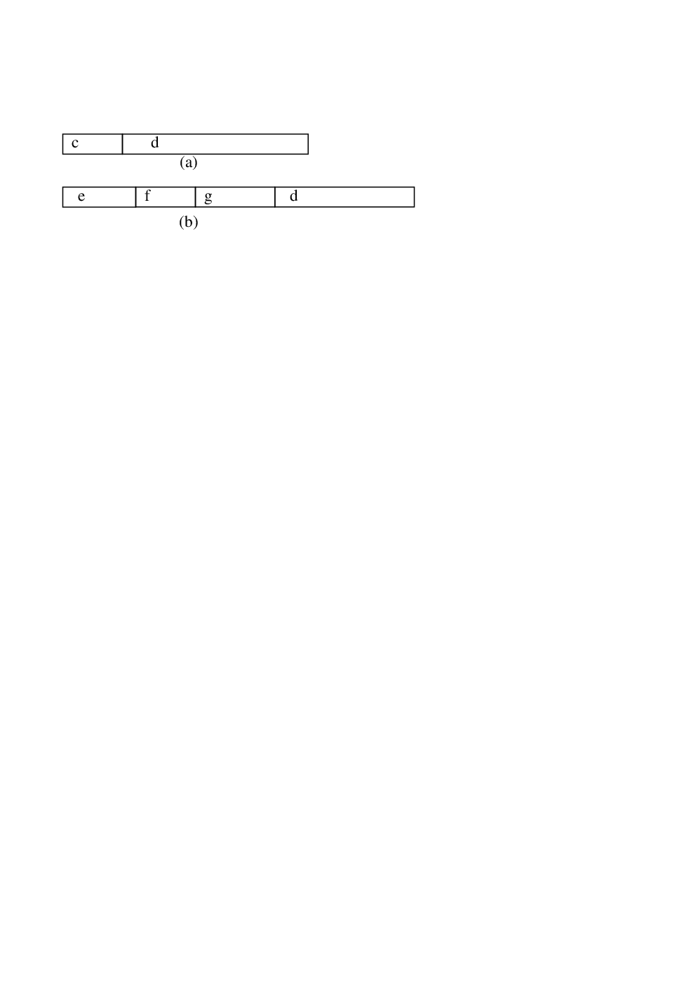
PR Transmission Protocol: We consider the conventional pilot-training-based transmission protocol for the PR, where the transmission of PR-Tx is divided into orthogonal time blocks, each of which is further divided into two sub-blocks: one contains the training signal and the other contains the data signal, as shown in Fig. 3(a). The training signal is for PR-Rx to estimate the PR channel as well as the received noise power (including the received CR interference power if ). It is assumed that these estimates are perfect since in this paper we focus on the deign of CR transmission. Based on the estimated and , PR-Rx computes the effective channel power gain , and according to designs a feedback signal for PR-Tx to adapt its transmit power and/or rate for the next block transmission (for simplicity, we assume that there is no delay or error for the PR feedback).
- •
CR Transmission Protocol: As shown in Fig. 3(b), the transmission protocol for the CR is more sophisticated than the conventional pilot-training-based one for the PR. Specifically, each CR block transmission consists of four stages: initial sensing, probing, re-sensing, and data transmission. For initial sensing, CR-Tx observes the received PR signal power and/or rate . Then, in the probing stage, CR-Tx transmits a predesigned signal of power to interfere with PR-Rx. The probing signal of CR-Tx can also be used as the training signal for CR-Rx. After that, CR-Tx goes into the re-sensing stage to observe the updated PR signal power and/or rate , and estimates according to the rule given in (15). Last, based on the estimated channel and the observed PR transmit adaptations, CR-Tx sets its transmit power and rate (details are given later in Section V), and starts data transmission.
Next, we discuss the following important issues for implementing the above CR transmission protocol based on active learning.
IV-B1 Time Synchronization
One important issue for the proposed scheme is the timing discrepancy between the distributed PR and CR links due to the lack of a common reference clock. Let , , and denote the propagation delays from PR-Tx to PR-Rx, from PR-Tx to CR-Tx, and from CR-Tx to PR-Rx, respectively, with . In addition, let denote the transmitted signal from PR-Tx. Then, the received signals at PR-Rx and CR-Tx are and (the channel multiplicative effect is ignored here since it is irrelevant to the discussion on time synchronization), respectively. Since CR-Tx does not have a common clock with PR-Tx, it has to use the received signal from PR-Tx as a reference clock. Hence, the transmitted probing signal from CR-Tx can be denoted as , where denotes the transmission time ahead of the reference clock (to be specified later). Accordingly, the received probing signal at PR-Rx is . Note that CR-Tx needs to make sure that its probing signal arrives at PR-Rx prior to the PR training signal in one particular transmission block, i.e., , to make an effective probing. Thus, it follows that . However, the exact values of , , and may not be known to CR-Tx. Instead, suppose that we know that the maximum propagation delay between CR and PR terminals is less than . Then, by setting , it is ensured that the CR probing signal arrives at PR-Rx prior to the PR training signal.
On the other hand, the duration of the probing signal from CR-Tx, denoted by , also needs to be properly designed. Note that in order to minimize the temporary performance degradation of the PR link due to the CR probing signal, it is desirable to choose a small value for . However, for the probing signal to be effective, it is also necessary to make sufficiently large such that the probing signal can overlap with the entire training signal of the PR at PR-Rx in one particular transmission block. Let denote the training signal duration of the PR, which is assumed known at CR-Tx. From the earlier discussion on time synchronization, we know that PR-Rx observes the PR signal, , and CR probing signal, . Thus, the maximal gap for the arrival time of the CR probing signal ahead of that of the PR training signal is when . Therefore, by setting , the aforementioned requirements for choosing are both fulfilled.
IV-B2 Rate Granularity
In the estimation rule given by (15), it has been assumed that the transmit rate of the PR, , is a continuous function of receiver SNR, . However, with practical MCSs, is usually a non-decreasing function of with a finite rate granularity, i.e., constituting only a finite number of discrete rate values. In this case, suppose that , with , , where denotes a discrete rate value, and and are corresponding SNR thresholds. In this case, although the CR cannot determine the exact value of from (15), it can safely estimate the range of this value as
| (22) |
IV-B3 Power Measurement Noise
Another assumption we have made on the estimation using (15) is that the sensor noise at CR-Tx is ignored for estimating the received PR signal powers, and , before and after the CR probing. In practice, only a finite number of PR signal samples can be obtained during the initial sensing and re-sensing periods at CR-Tx, which are corrupted by the receiver noise. For convenience, we assume that the noise power at CR-Tx is , the same as that at CR-Rx, and is known to CR-Tx. Also assume that independent signal samples are obtained during both the initial sensing and re-sensing periods at CR-Tx, denoted by , . Specifically, we have
| (23) |
where denotes the PR signal component, with , and ’s are independent Gaussian noises with zero mean and variance of . Instead of having the exact values for and , we can obtain their estimated values as follows.
| (24) |
According to the central limit theorem [25], if the number of samples is large enough (e.g., in practice), the above estimation statistics are asymptotically normally distributed with corresponding mean
| (25) |
and variance
| (26) |
Since ’s are unknown at CR-Tx, the exact values of ’s are not available at CR-Tx. However, if it is known that the PR transmit powers must be below a prescribed maximum value, denoted by , the upper bounds for ’s can be obtained as
| (27) |
Thus, it follows that
| (28) | ||||
| (29) |
where is the complementary cumulative distribution function [25], and is a design parameter. Similarly, we have
| (30) |
In other words, we have a belief in probability of at least for and . Accordingly, from (15), it follows that with a probability of at least
| (31) |
Similarly, with the same probability guarantee, we have
| (32) |
Note that in (31) and (32), we have assumed that and , respectively. Thus, even with a finite number of observation samples corrupted by additive noises, CR-Tx can still obtain a pair of upper and lower bounds on with a large belief probability (by setting a sufficiently large value for ). However, if the chosen is too large, it also increases the uncertainty range for the estimation.
IV-B4 Channel Variation
Last, we address the issue on possible channel variations during the implementation of the proposed CR active learning scheme. It is worth noting that the assumption of constant channels has usually been made in prior works (see, e.g., [21, 22, 23]) on iterative user power/rate adaptations in decentralized multiuser systems. From the proof of Proposition IV.1, we see that if the channel power gain, , through which CR-Tx estimates the received signal powers and from PR-Tx, changes from the initial sensing stage to the re-sensing stage, the estimation result will get affected. Let and denote the true values of during the initial sensing and re-sensing periods, respectively. We can rewrite the estimation rule in (15) as (assuming the perfect rate and power estimation)
| (33) |
Although CR-Tx does not know the exact values of and , it can predict the approximate range for their ratio given the channel coherence time relative to the time interval between the initial sensing and re-seining stages, and obtain the corresponding upper and lower bounds on the estimated value from (33). Furthermore, the channel power gain from CR-Tx to PR-Rx may also change from the probing stage to the data transmission stage. Similarly as for , given the channel coherence time and the time interval between these two stages, CR-Tx can estimate the range of accordingly.
V Supervised Transmission
In the previous section, we have proposed an active learning scheme for the CR to estimate the channel gain from CR-Tx to PR-Rx by exploiting the hidden PR feedback. In this section, we design supervised transmission for CR data transmission stage shown in Fig. 3(b), based on the acquired knowledge from active learning. In the following, we address two main design objectives for CR supervised transmission: controlling the PR link performance degradation and maximizing the CR link throughput.
V-A PR Performance Loss Control
In this subsection, we illustrate how to apply the estimated CR-to-PR channel gain from active learning for CR-Tx to predict the performance loss of the PR link due to CR data transmission. For simplicity, we assume that the estimation of is perfect at CR-Tx, although the obtained results can be easily extended to the case of imperfect channel estimation by utilizing the derived estimation bounds in Section IV-B. We consider two general types of performance losses for the PR link: One is for the case where the PR employs variable-rate transmission (e.g., with CP or WF power control), named as rate penalty, which measures the PR rate loss due to the CR interference, expressed as , where denotes the resultant PR transmit rate in the CR data transmission stage; the other is for the case where the PR employs constant-rate transmission (e.g., with TCI power control), named as power penalty, which measures the additional transmit power in dB required for the PR to maintain the prescribed constant rate under the CR interference, expressed as , where denotes the resultant PR transmit power in the CR data transmission stage. Note that and denote the PR transmit rate and power without the CR interference, respectively, in the CR initial sensing stage. Let denote the CR transmit power in the data transmission stage.
First, the rate penalty for the PR link can be more explicitly expressed as
| (34) |
Note that for the convenience of analysis, we have assumed the “SNR gap approximation” that accounts for the rate loss from the optimal capacity due to practical/non-Gaussian MCS employed by the PR [26], i.e., , where denotes the constant SNR gap for the PR.
In the case of CP policy for the PR, from (34) it follows that
| (35) | ||||
| (36) | ||||
| (37) |
Therefore, CR-Tx knows that if it transmits with power , the resultant rate loss of the PR is upper-bounded by the value given in (37), which depends on the estimated , but is independent of the PR transmit power and SNR gap .
Consider next the case of WF power control for the PR similarly as that given in (III) but with therein replaced by . In this case, assuming that (otherwise the rate penalty for the PR is trivially zero), from (34) can be further expressed as
| (38) |
It thus follows that
Thus, CR-Tx can predict the exact rate loss of the PR as a function of , based on the estimated and from the active learning.
Last, consider the power penalty of the PR with the TCI power control given in (III). Assuming that , i.e., the CR interference power is not sufficiently large to render the PR into a transmit outage (otherwise the power penalty of the PR becomes irrelevant), it thus follows that
| (42) |
Thus, CR-Tx can measure the power penalty of the PR as a function of .
From the above discussions, we see that the derived rate and power penalties enable CR-Tx to predict quantitatively the resultant PR performance losses corresponding to different transmit power levels of the CR, using only the observed/estimated parameters from the active learning.
V-B CR Achievable Rate
In the previous subsection, we have shown for the CR supervised transmission how to control the resultant PR link performance degradation. With a given PR rate/power penalty, CR-Tx can derive accordingly the maximum tolerable transmit power . In this subsection, we analyze the CR link achievable rate as a function of . Due to the space limitation, we consider only the case of single-user detection at CR-Rx for decoding the CR message, by treating the interference from PR-Tx as additive noise. However, it is worth noting that more advanced multiuser detection techniques can be employed at CR-Rx to decode both the CR and PR messages in order to suppress the PR interference (details are omitted here; the interested readers may refer to a preliminary version of this paper [27]).
With single-user detection, the achievable rate of the CR link in the data transmission stage can be expressed as
| (43) |
where denotes the SNR gap for the CR, and
| (44) |
with denoting the PR employed power control policy (e.g., CR, TCI, or WF). It is interesting to observe that in general the CR achievable rate is related to the CR transmit power not only through the direct link from CR-Tx to CR-Rx, but also through the interference link from CR-Tx to PR-Rx, the resultant PR power adaptation and “feedback” interference from PR-Tx to CR-Rx. Thus, CR-Tx is able to control the interference power from PR-Tx by changing transmit power via the hidden PR feedback.
With the PR feedback interference, some interesting observations can be drawn for the CR achievable rate as a function of . Note that without the PR interference, is an increasing function of . However, with the PR feedback interference, the interference power from PR-Tx can also be an increasing function of in the case of persistent power control for the PR (e.g., TCI). As a result, it is unclear in this case whether increasing the CR transmit power will result in a net gain for its achievable rate. Thus, it is pertinent to investigate further on for the CR link under the PR feedback interference, as shown in the following proposition.
Proposition V.1
For any under which with is a positive, continuous and differentiable function of , if and only if , where
| (45) |
The proof of Proposition V.1 follows from (43) and is thus omitted here for brevity. It is noted that CP and WF power control policies for the PR satisfy the condition given in Proposition V.1 straightforwardly, since they are both non-persistent power control. For the TCI power control of the CR which is persistent, it can be verified (details are omitted here for brevity) that , for all values of as required in Proposition V.1. It thus follows that is a strictly increasing function of in all cases of CP, WF, or TCI power control policies for the PR.
VI Numerical Examples
In this section, we present numerical examples to validate the effectiveness of our proposed schemes for CR active learning and supervised transmission. It is assumed that and in Fig. 1. For simplicity, we assume that all these channels are constant over the PR and CR transmission blocks where the proposed CR schemes are implemented. We evaluate the performance for the CR-to-PR channel gain estimation based on active learning, as well as the PR performance degradation control and CR achievable rate with CR supervised transmission. We consider the following two scenarios: Case I: the PR employs a constant-power (CP) variable-rate transmission; and Case II: the PR employs a constant-rate variable-power (with TCI power control) transmission. For convenience, we assume that , and .
Consider first Case I, where the PR transmits with a constant power . In this case, we are interested in investigating the effects of finite rate granularity for the PR variable-rate transmission on the performances of the CR active learning and supervised transmission. Suppose that the PR transmit rate for a given effective channel gain is expressed as
| (46) |
in bps/Hz, where denotes the floor operation; and denotes the “bit granularity” due to the fact that practical MCS only supports a finite set of discrete transmit rates corresponding to integer multiplications of . We assume that dB and (i.e., one-bit granularity). From (22), it follows that the upper and lower bounds on in the case of one-bit granularity are obtained as
| (47) |
where and denote the discrete rates of the PR observed by the CR in the sensing and re-sensing stages, respectively. In Fig. 4(a), we show the estimated upper and lower bounds for using the above estimation rule. It is observed that with small value of CR probing signal power , the gap between the estimated upper and lower bounds for is large, suggesting that the estimation of is not accurate. This is due to the fact that if is too small, the interference at PR-Rx is not sufficiently strong to make the PR reduce its transmit rate by at least one bit (Note that ), and as a result, the CR observes the same value of as . However, with larger value of , the CR is able to make and thus obtain a more accurate estimation for . Thus, there is in general a tradeoff between minimizing the PR performance degradation and the CR-to-PR channel estimation error for the CR active learning. In Fig. 4(b) and 4(c), we show the PR rate penalty and CR achievable rate, respectively, vs. CR transmit power for CR supervised data transmission. It is observed that both the PR rate penalty and CR transmit rate increase with . Moreover, in Fig. 4(b), we compare the actual resultant PR rate penalty (with one-bit granularity) to its estimated value using (37) and the estimated upper bound on from active learning with . It is observed that the estimated PR rate penalties are indeed valid upper bounds on their true values for different values of .
It is worth comparing the spectrum-sharing performance for the PR and CR links with the proposed active learning and supervised transmission for the CR, with the approach (refereed to as “No Feedback”) without exploiting the PR hidden feedback, or the approach (refereed to as “Perfect Feedback”) with the perfect knowledge of the CR-to-PR channel via a dedicated feedback channel from PR-Rx to CR-Tx. Note that for all three design approaches, the achievable rates for the CR with a given transmit power are identical, as shown in Fig. 4(c). However, the main differences among these designs are highlighted as follows. For the case of “No Feedback”, the CR has no means to predict the PR performance loss as a function of and thus cannot deploy any opportunistic transmission; as a result, the CR has to transmit constantly with a very low power and thus results in low spectral efficiency. In contrast, with the new proposed design, the CR can always predict its maximum transmit power given the PR transmission margin and decide its transmit rate accordingly. On the other hand, for the case of “Perfect Feedback”, as shown in Fig. 4(b), for a given PR rate penalty value, the CR with the perfect channel knowledge can transmit with a larger power than the proposed design with active learning based channel estimation, and thus the maximum achievable rate for the CR also becomes larger (cf. Fig. 4(b) & 4(c)).
Next, consider Case II, where the PR transmits with a constant rate or equivalently maintains a constant receiver SNR, . Thus, the TCI power control given in (III) is used by the PR with . In this case, we are interested in investigating the effects of a finite number of observation samples and receiver noise at CR-Tx for estimating the received PR signal powers on the performances of CR active learning and supervised transmission. From (31) and (32), it follows that the upper and lower bounds on in the case of a finite number of observed PR signal samples are obtained as
| (48) |
where and denote the observed powers at CR-Tx in the sensing and re-sensing stages, respectively. In order to keep the estimated within the above range with a probability guarantee of , we choose since . Furthermore, we set and for determining the constant defined in (27). In Fig. 5(a), we show the estimated upper and lower bounds for using the above rule. Similar to our previous observations for Fig. 4(a), it is observed that the CR probing power needs to be sufficiently large in order to make a reasonably good estimate on . In Fig. 5(b) and 5(c), we show the PR power penalty and CR achievable rate, respectively, vs. CR transmit power for CR supervised data transmission. It is observed that both the PR power penalty and CR transmit rate increase with . Moreover, in Fig. 5(b), we compare the actual PR power penalty to its estimated value using (42) and the estimated upper bound on from active learning with . It is observed that the estimated PR power penalties are valid upper bounds on the true values, which become tighter for smaller values of . Comparing the CR achievable rates in Fig. 4(c) and Fig. 5(c), it is observed that the CR rate increase with is much slower in the latter than the former case. This is because for Fig. 5(c), the PR employs TCI power control instead of CP as for Fig. 4(c), and thus the PR feedback interference power at CR-Rx increases with instead of being a constant as for the case of Fig. 4(c) with CP.
VII Conclusion
This paper introduces a new design paradigm for spectrum sharing based CRs, where the CR designs its learning and transmission from the observed PR transmit power/rate adaptations upon receiving a probing signal from the CR, namely the hidden PR feedback. First, a novel active learning scheme is proposed for the CR to estimate the channel gain from its transmitter to the PR receiver, which is essential for the CR interference control to the PR. Second, with the acquired channel knowledge and PR transmit adaptations from active learning, the CR supervised data transmission is designed by effectively controlling the performance degradation of the PR as a function of the CR transmit power. Moreover, this paper shows that the CR is able to predict its own achievable rate under the PR feedback interference, which is coupled with the CR transmit power via the hidden PR feedback. This paper presents a new transmission protocol for the CR to implement the proposed learning and transmission schemes, and proposes the solutions to deal with various important practical issues. The results in this paper provide a new promising approach to interference management for decentralized multiuser communication systems.
References
- [1] S. Haykin, “Cognitive radio: brain-empowered wireless communications,” IEEE J. Sel. Areas Commun., vol. 23, no. 2, pp. 201-220, Feb. 2005.
- [2] N. Devroye, P. Mitran, and V. Tarokh, “Achievable rates in cognitive radio channels,” IEEE Trans. Inf. Theory, vol. 52, no. 5, pp. 1813-1827, May 2006.
- [3] A. Joviĉić and P. Viswanath, “Cognitive radio: an information-theoretic perspective,” IEEE Trans. Inf. Theory, vol. 55, no. 9, pp. 3945-3958, Sep. 2009.
- [4] R. Zhang, Y. C. Liang, and S. Cui, “Dynamic resource allocation in cognitive radio networks: a convex optimization perspective,” IEEE Sig. Process. Mag., vol. 27, no. 3, pp. 102-114, May 2010.
- [5] M. Gastpar, “On capacity under receive and spatial spectrum-sharing constraints,” IEEE Trans. Inf. Theory, vol. 53, no. 2, pp. 471-487, Feb. 2007.
- [6] A. Ghasemi and E. S. Sousa, “Fundamental limits of spectrum-sharing in fading environments,” IEEE Trans. Wireless Commun., vol. 6, no. 2, pp. 649-658, Feb. 2007.
- [7] L. Musavian and S. Aissa, “Capacity and power allocation for spectrum-sharing communications in fading channels,” IEEE Trans. Wireless Commun., vol. 8, no. 1, pp. 148-156, Jan. 2009.
- [8] X. Kang, Y. C. Liang, A. Nallanathan, H. Garg, and R. Zhang, “Optimal power allocation for fading channels in cognitive radio networks: ergodic capacity and outage capacity,” IEEE Trans. Wireless Commun., vol. 8, no. 2, pp. 940-950, Feb. 2009.
- [9] R. Zhang and Y. C. Liang, “Exploiting multi-antennas for opportunistic spectrum sharing in cognitive radio networks,” IEEE J. Sel. Topics Sig. Process., vol. 2, no. 1, pp. 88-102, Feb. 2008.
- [10] R. Zhang, “Optimal power control over fading cognitive radio channels by exploiting primary user CSI,” in Proc. IEEE Global Commun. Conf. (Globecom), Dec. 2008.
- [11] R. Zhang, “On peak versus average interference power constraints for protecting primary users in cognitive radio networks,” IEEE Trans. Wireless Commun., vol. 8, no. 4, pp. 2112-2120, Apr. 2009.
- [12] K. Eswaran, M. Gastpar, and K. Ramchandran, “Bits through ARQs: spectrum sharing with a primary packet system,” in Proc. IEEE Int. Symp. Inf. Theory (ISIT), pp. 2171-2175, June 2007.
- [13] Y. Chen, G. Yu, Z. Zhang, H. H. Chen, and P. Qiu, “On cognitive radio networks with opportunistic power control strategies in fading channels,” IEEE. Trans. Wireless Commun., vol. 7, no. 7, pp. 2752-2761, July 2008.
- [14] R. Zhang, F. Gao, and Y. C. Liang, “Cognitive beamforming made practical: effective interference channel and learning-throughput tradeoff,” IEEE Trans. Commun., vol. 58, no. 2, pp. 706-718, Feb. 2010.
- [15] W. Zhang and U. Mitra, “A spectrum-shaping perspective on cognitive radio: uncoded primary transmission case,” in Proc. IEEE Int. Symp. Inf. Theory (ISIT), July 2008.
- [16] X. Kang, R. Zhang, Y. C. Liang, and H. K. Garg, “Optimal power allocation for cognitive radio under primary user outage capacity constraint,” in Proc. IEEE Int. Conf. Commun. (ICC), June 2009.
- [17] C. Cordeiro, K. Challapali, D. Birru, and N. S. Shankar, “IEEE 802.22: the first worldwide wireless standard based on cognitive radios,” in Proc. IEEE Symp. New Frontiers in Dynamic Spectrum Access Networks (DySPAN), pp. 328-337, Nov. 2005.
- [18] V. Chandrasekhar, J. Andrews, and A. Gatherer, “Femtocell networks: a survey,” IEEE Communications Magazine, vol. 48, no. 9, pp. 59-67, Sep. 2008.
- [19] R. Zhang and Y. C. Liang, “Exploiting hidden power feedbacks in cognitive radio networks,” in Proc. IEEE Int. Symp. New Frontiers in Dynamic Spectrum Access Networks (DySPAN), Oct. 2008.
- [20] G. Zhao, Y. (G.) Li, and C. Yang, “Proactive detection of spectrum holes in cognitive radio,” in Proc. IEEE Int. Conf. Commun. (ICC), June 2009.
- [21] G. J. Foschini, “A simple distributed autonomous power control algorithm and its convergence,” IEEE Trans. Veh. Technol., vol. 42, pp. 641-646, Nov. 1993.
- [22] R. D. Yates, “A framework for uplink power control in cellular radio systems,” IEEE J. Sel. Areas Commun., vol. 13, no. 7, pp. 1341-1347, Sep. 1995.
- [23] W. Yu, G. Ginis, and J. Cioffi “Distributed multiuser power control for digital subscriber lines,” IEEE J. Sel. Areas Commun., vol. 20, no. 5, pp. 1105-1115. June 2002.
- [24] A. Goldsmith and P. P. Varaiya, “Capacity of fading channels with channel side information,” IEEE Trans. Inf. Theory, vol. 43, no. 6, pp. 1986-1992, Nov. 1997.
- [25] A. Papoulis, Probability, random variables, and stochastic processes, 2nd ed. New York: McGraw-Hill, 1984.
- [26] T. Starr, J. M. Cioffi, and P. J. Silverman, Understanding digital subscriber line technology, Englewood Cliffs, NJ: Prentice-Hall, 1999.
- [27] R. Zhang, “On active learning and supervised transmission of spectrum sharing based cognitive radios by exploiting hidden primary radio feedback,” in Proc. IEEE Global Commun. Conf. (Globecom), Dec. 2009.