Learning Nonlinear Dynamic Models

John Langford Address: Yahoo! Research, New York, NY 10011 Ruslan Salakhutdinov Address: Department of Computer Science, University of Toronto, Ontario M2N6T3 Tong Zhang Address: Department of Statistics, Rutgers University, Piscataway, NJ 08854

Abstract

We present a novel approach for learning nonlinear dynamic models, which leads to a new set of tools capable of solving problems that are otherwise difficult. We provide theory showing this new approach is consistent for models with long range structure, and apply the approach to motion capture and high-dimensional video data, yielding results superior to standard alternatives.

1 Introduction

The notion of hidden states appears in many nonstationary models of the world such as Hidden Markov Models (HMMs), which have discrete states, and Kalman filters, which have continuous states. Figure 1 shows a general dynamic model with observation ${\bf x}_{t}$ and unobserved hidden state ${\bf y}_{t}$ . The system is characterized by a state transition probability $P({\bf y}_{t+1}|{\bf y}_{t})$ , and a state to observation probability $P({\bf x}_{t}|{\bf y}_{t})$ .

The method for predicting future events under such a dynamic model is to maintain a posterior distribution over the hidden state ${\bf y}_{t+1}$ , based on all observations $X_{1:t}=\{{\bf x}_{1},\ldots,{\bf x}_{t}\}$ up to time $t$ . The posterior can be updated using the formula:

		$\displaystyle P({\bf y}_{t+1}\|X_{1:t})$
		$\displaystyle\quad\propto\sum_{{\bf y}_{t}}P({\bf y}_{t}\|X_{1:{t-1}})P({\bf x}_{t}\|{\bf y}_{t})P({\bf y}_{t+1}\|{\bf y}_{t}).$		(1)

The prediction of future events ${\bf x}_{t+1},\ldots,{\bf x}_{t+k}$ , $k>0$ , conditioned on $X_{1:t}$ is through the posterior over ${\bf y}_{t}$ :

		$\displaystyle P({\bf x}_{t+1},\ldots,{\bf x}_{t+k}\|{\bf x}_{1:t})$
		$\displaystyle\quad\propto P({\bf y}_{t+1}\|X_{1:t})P({\bf x}_{t+1},\ldots,{\bf x}_{t+k}\|{\bf y}_{t+1}).$		(2)

Hidden state based dynamic models have a wide range of applications, such as time series forecasting, finance, control, robotics, video and speech processing. Some detailed dynamic models and application examples can be found in (WestHarr97).

From Eq. 2, it is clear that the benefit of using a hidden state dynamic model is that the information contained in the observation $X_{1:t}$ can be captured by a relatively small hidden state ${\bf y}_{t+1}$ . Therefore in order to predict the future, we do not have to use all previous observations $X_{1:t}$ but only its state representation ${\bf y}_{t+1}$ . In principle, ${\bf y}_{t+1}$ may contain a finite history of length $k+1$ , such as ${\bf x}_{t},{\bf x}_{t-1},\ldots,{\bf x}_{t-k}$ . Although the notation only considers first order dependency, it incorporates higher order dependency by considering a representation of the form $Y_{t}=[{\bf y}_{t}^{\prime},{\bf y}_{t-1}^{\prime},\ldots,{\bf y}_{t-k}^{\prime}]$ , which is a standard trick.

Refer to caption — Figure 1: Dynamic Model with observation vector ${\bf x}_{t}$ and hidden state vector ${\bf y}_{t}$ .

In an HMM or Kalman filter, both transition and observation functions are linear maps. There are reasonable algorithms that can learn these linear dynamic models. For example, in addition to the classical EM approach, it was recently shown that global learning of certain hidden Markov models can be achieved in polynomial time (Linear). Moreover, for linear models, the posterior update rule is quite simple. Therefore, once the model parameters are estimated, such models can be readily applied for prediction.

However in many real problems, the system dynamics cannot be approximated linearly. For such problems, it is often necessary to incorporate nonlinearity into the dynamic model. The standard approach to this problem is through nonlinear probability modeling, where prior knowledge is required to define a sensible state representation, together with parametric forms of transition and observation probabilities. The model parameters are learned by using probabilistic methods such as the EM (WB; RG). When the learned model is applied for prediction purposes, it is necessary to maintain the posterior $P({\bf y}_{t}|X_{1:t})$ using the update formula in Eq. 1. Unfortunately, for nonlinear systems, maintaining $P({\bf y}_{t}|{\bf x}_{1:t})$ is generally difficult because the posterior can become exponentially more complex (e.g., exponentially many mixture components in a mixture model) as $t$ increases.

This computational difficulty is a significant obstacle to applying nonlinear dynamic systems to practical problems. The traditional approach to address the computational difficulty is through approximation methods. For example, in the particle filtering approach (GSS93; Arulampalam2002), one uses a finite number of samples to represent the posterior distribution and the samples are then updated as observations arrive. Another approach is to maintain a mixture of Gaussians to approximate the posterior, $P({\bf y}_{t}|X_{1:t})$ , which may also be regarded as a mixture of Kalman filters (ChenLiu00). Although an exponential in $t$ number of mixture components are needed to accurately represent the posterior, in practice, one has to use a fixed number of mixture components to approximate the distribution. This leads to the following question: even if the posterior can be well-approximated by a computationally tractable approximation family (such as finite mixtures of Gaussians), how can one design a good approximate inference method that is guaranteed to find a good quality approximation? The use of complex techniques required to design reasonable approximation schemes makes it non-trivial to apply nonlinear dynamic models for many practical problems.

This paper introduces an alternative approach, where we start with a different representation of a linear dynamic model which we call the sufficient posterior representation. It is shown that one can recover the underlying state representation by using prediction methods that are not necessarily probabilistic. This allows us to model nonlinear dynamic behaviors with many available nonlinear supervised learning algorithms such as neural networks, boosting, and support vector machines in a simple and unified fashion. Compared to the traditional approach, it has several distinct advantages:

•

It does not require us to design any explicit state representation and probability model using prior knowledge. Instead, the representation is implicitly embedded in the representational choice of the underlying supervised learning algorithm, which may be regarded as a black box with the power to learn an arbitrary representation. The prior knowledge can be simply encoded as input features to the learning algorithms, which significantly simplifies the modeling aspect.
•

It does not require us to come up with any specific representation of the posterior and the corresponding approximate Bayesian inference schemes for posterior updates. Instead, this issue is addressed by incorporating the posterior update as part of the learning process. Again, the posterior representation is implicitly embedded in the representational choice of the underlying supervised learning algorithm. In this sense, our scheme learns the optimal representation for posterior approximation and the corresponding update rules within the representational power of the underlying supervised algorithm¹¹ 1 Many modern supervised learning algorithms are universal, in the sense that they can learn an arbitrary representation in the large sample limit..
•

It is possible to obtain performance guarantees for our algorithm in terms of the learning performance of the underlying supervised algorithm. The performance of the latter has been heavily investigated in the statistical and learning theory literature. Such results can thus be applied to obtain theoretical results on our methods for learning nonlinear dynamic models.

2 Sufficient Posterior Representation

Instead of starting with a probability model, our approach directly attacks the problem of predicting ${\bf y}_{t+k}$ based on $X_{1:t}$ . Clearly the prediction depends only on the posterior distribution $P({\bf y}_{t+1}|X_{1:t})$ . Therefore we can solve the prediction problem as long as we can estimate, and update this posterior distribution.

In our approach, it is assumed that the posterior $P({\bf y}_{t+1}|X_{1:t})$ can be approximated by a family of distributions parameterized by ${\bf s}_{t+1}\in{\cal S}$ : $P({\bf y}_{t+1}|X_{1:t})\approx P({\bf y}_{t+1}|{\bf s}_{t+1})$ for some deterministic parameter ${\bf s}_{t+1}$ that depends on $X_{1:t}$ . That is, ${\bf s}_{t+1}$ is a sufficient statistic for the posterior $P({\bf y}_{t+1}|X_{1:t})$ , and updating the posterior is equivalent to updating the sufficient statistic ${\bf s}_{t+1}$ . The augmented model that incorporates the (approximate) sufficient statistics ${\bf s}_{t}\in{\cal S}$ is shown in Fig. 2. In this model, ${\bf y}_{t}$ can be integrated out, which leaves a model containing only ${\bf s}_{t}$ and ${\bf x}_{t}$ .

According to the posterior update of Eq. 1, there exists a deterministic function $B$ such that:

{\bf s}_{{t+1}}=B({\bf x}_{t},{\bf s}_{t}).

For simplicity, we can give an arbitrary value for the initial state ${\bf s}_{1}$ , and let:

{\bf s}_{2}=A({\bf x}_{1})=B({\bf x}_{1},{\bf s}_{1}).

Moreover, according to Eq. 2, given an arbitrary vector function $f$ of the future events $X_{t+1:\infty}=\{{\bf x}_{t+1},{\bf x}_{t+2},\cdots\}$ , there exists a deterministic function $C^{f}$ ( $k>0$ ) such that:

E_{X_{t+1:\infty}}[f(X_{t+1:\infty})|X_{1:t}]=C^{f}({\bf s}_{t+1}).

Therefore the dynamics of the model in Fig. 1 is determined by the posterior initialization rule $A$ and posterior update rule $B$ . Moreover, the prediction of the system is completely determined by the function $C^{f}$ .

The key observation of our approach is that the functions $A$ , $B$ , and $C$ are deterministic, which does not require any probability assumption. It fully captures the correct dynamics of the underlying probabilistic dynamic model. However, by removing the probability assumption, we obtain a more general and flexible model. In particular, we are not required to start with specific forms of the transition model $P({\bf y}_{t+1}|{\bf y}_{t})$ , the observation model $P({\bf x}_{t}|{\bf y}_{t})$ , or the posterior sufficient statistic model $P({\bf y}_{t+1}|{\bf x}_{1:t})\approx P({\bf y}_{t+1}|{\bf s}_{t+1})$ , as required in the standard approach. Instead, we may embed the forms of such models into the functional approximation forms in standard learning algorithms, such as neural networks, kernel machines, or tree ensembles. These are universal learning machines that are well studied in the learning theory literature.

Our approach essentially replaces a stochastic hidden state representation through the actual state $Y$ by a deterministic representation through the posterior sufficient statistic $S$ . Although the corresponding representation may become more complex (which is why in the traditional approach, ${\bf y}_{t}$ is always explicitly included in the model), this is not a problem in our approach, because we do not have to know the explicit representation. Instead, the complexity is incorporated into the underlying learning algorithm — this allows us to take advantage of sophisticated modern supervised learning algorithms that can handle complex functional representations. Moreover, unlike the traditional approach, in which one designs a specific form of $P({\bf y}_{t}|{\bf s}_{t})$ by hand, and then derives an approximate update rule $B$ by hand using Bayesian inference methods, here, we simply use learning to come up with the best possible representation and update (assuming the underlying learning algorithm is sufficiently powerful). We believe this approach is also more robust because it is less sensitive to model mis-specifications or non-optimal approximate inference algorithms that commonly occur in practice.

By changing the standard probabilistic dynamic model in Fig. 1 to its sufficient posterior representation in Fig. 2 (where we assume ${\bf y}_{t}$ is integrated out, and thus can be ignored), we can define the goal of our learning problem. Since ${\bf y}_{t}$ is removed from the formulation, in the following, we shall refer to the sufficient posterior statistic ${\bf s}_{t}$ simply as state.

We can now introduce the following definition of Sufficient Posterior Representation of Dynamic Model, which we refer to SPR-DM.

Definition 2.1.

(SPR-DM) A sufficient posterior representation of a dynamic model is given by an observed sequence $\{{\bf x}_{t}\}$ and unobserved hidden state $\{{\bf s}_{t}\}$ , characterized by state initialization map ${\bf s}_{2}=A({\bf x}_{1})$ , state update map ${\bf s}_{t+1}=B({\bf x}_{t},{\bf s}_{t})$ , and state prediction maps:

E_{X_{t+1:\infty}}[f(X_{t+1:\infty})|X_{1:t}]=C^{f}({\bf s}_{t+1})

for any pre-determined vector function $C^{f}$ .

Our goal in this model is to learn the model dynamics characterized by $A$ and $B$ , as well as $C^{f}$ for any given vector function of interest.

3 Learning SPR-DM

The essential idea of our algorithm is to use a bottlenecking approach to construct an implicit definition of state, along with state space evolution and projection operators to answer various natural questions we might pose.

3.1 Training

There are two parts to understanding the training process. The first is the architecture trained, and the second is the exact method of training this architecture. Note that our architecture is essentially functional rather than representational.

3.1.1 Architecture

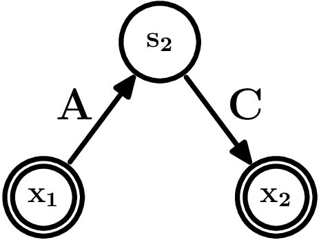
Graphically, in order to recover the system dynamics, we solve two distinct kinds of prediction problems. To understand these graphs it is essential to understand that the arrows do not represent graphical models. Instead, they are a depiction of which information is used to predict which other information. We distinguish observations and hidden “state” as double circles and circles respectively, to make clear what is observed and what is not.

The first prediction problem solved in Fig. 3, left panel, provides our initial definition of state. Essentially, state is “that information which summarizes the first observation in predicting the second observation”. Compared to a conventional dynamic model, the quantity ${\bf s}_{2}$ may be a sufficient statistic of the state posterior after integrating $x_{1}$ , the posterior after integrating $x_{1}$ and evolving one step or some intermediate mixture. This ambiguity is fundamental, but inessential.

The second prediction problem is state evolution, shown in Fig. 3, middle panel. Here, we use a state and an observation to predict the next state, reusing the prediction of state from observation from the first step. Note that even though there are two sources of information for predicting ${\bf s}_{t}$ , only one prediction problem (using both sources) is solved. Operator $B$ is what is used to integrate new information into the state of an online system.

Without loss of generality, in the notation of Fig. 3 we consider $f_{0}(X_{t+1:\infty})=E[{\bf x}_{t+1}|X_{1:t}]$ , and denote $C^{f_{0}}$ by $C$ . An alternative interpretation of $C$ , which we do not distinguish in this paper, is to learn the probability distribution over ${\bf x}_{t+1}$ . It should be understood that our algorithm can be applied with other choices of $f_{0}$ .

The above two learning diagrams are used to obtain the system dynamics ( $A$ and $B$ ). One can then use the learned system dynamics to learn prediction rules $C^{f}$ with any function $f$ of interest. Here, we consider the problem of predicting ${\bf x}_{t+k}$ at different ranges of $k=2^{j}$ . This gives a state projection operator $D_{j}:{\bf s}_{t}\to{\bf s}_{t+2^{j}}$ , without observing the future sequence ${\bf x}_{t+1},{\bf x}_{t+2},\cdots$ . The learning of state projection is presented in Fig. 3, right panel. The idea in state projection is that we want to build a predictor of the observation far in the future. To do this, we’ll chain together several projection operators from the current state. To make the system computationally more efficient, we learn $\left\lfloor\log_{2}T\right\rfloor$ operators, each specialized to cover different timespans. Note that state evaluation provides an efficient way to learn ${\bf x}_{t+k}$ based on ${\bf s}_{t}$ simultaneously for multiple $k$ through combination of projection operators. If computation is not an issue, one may also learn ${\bf x}_{t+k}$ based on ${\bf s}_{t}$ separately for each $k$ .

3.1.2 Method

Training of $A$ is straightforward. Training of $C$ is complicated by the fact that samples appear at multiple timesteps, but otherwise straightforward given the other components. To deal with multiple timesteps, it is important for our correctness proof in section 4.2 that the observation ${\bf x}_{t}$ include the timestep $t$ . The training of $D$ is also straightforward given everything else (and again, we’ll require the timestep be a part of the update for the correctness proofs).

The most difficult thing to train is $B$ , since an alteration to $B$ can cascade over multiple timesteps. The method we chose takes advantage of both local and global information to provide a fast near-optimal solution.

1.

Initialization: Learn $B_{t},C_{t}$ starting from timestep $t=1$ and conditioning on the previous learned value. Multitask learning or initialization with prior solutions may be applied to improve convergence here. In our experiments, we initialize $B_{t},C_{t}$ to the average parameter values of previous timesteps and use stochastic gradient descent techniques for learning.
2.

Conditional Training Learn an alteration $B^{\prime}$ which optimizes performance given that the existing $B_{t}$ are used at every other time step. Since computational performance is an issue, we use a “backprop through time” gradient descent style algorithm. For each timestep $t$ , we compute the change in squared loss for all future observations using the chain rule, and update according to the negative gradient.
3.

Iteration: Update $B$ using stochastic mixing according to $B_{i}=\alpha B^{\prime}+(1-\alpha)B_{i-1}$ where $\alpha$ is the stochastic mixing parameter. The precise method of stochastic mixing used in the experiments is equivalent to applying the derivative update with probability $\alpha$ and not update with probability $1-\alpha$ , which is a computational and representational improvement over Searn (Searn).

We prove (below) that the method in step (1) alone is consistent. Steps (2) and (3) are used to force convergence to a single $B$ and $C$ while retaining the performance gained in step (1). The intuition behind step (3) is that when $\alpha=o(\frac{1}{T})$ , with high probability $B^{\prime}$ is executed only once, implying that $B^{\prime}$ need only perform well with respect to the learning problem induced by the rest of the system to improve the overall system. This approach was first described in Conservative Policy Iteration (CPI).

3.2 Testing

We imagine testing the algorithm by asking questions like: what is the probability of observation ${\bf x}_{t^{\prime}}$ given what is known up to time $t$ for $t^{\prime}>t$ ? This is done by using $A({\bf x}_{1})$ to get ${\bf s}_{2}$ , then using $B({\bf x}_{i},{\bf s}_{i})$ to evolve the state to ${\bf s}_{t}$ . Then the time interval from $t^{\prime}-t$ is broken down into factors of $2$ , and the corresponding state projection operators $D_{i}$ are applied to the state resulting in a prediction for ${\bf s}_{t^{\prime}-1}$ . This is transformed into a prediction for ${\bf x}_{t^{\prime}}$ using operator $C$ .

4 Analysis

4.1 Computation

The computational requirements depend on the exact training method used. For the initialization step, training of $A$ , $B_{t}$ , and $C_{t}$ requires just $O(nT)$ examples. Training $D_{i}$ can be done with just $O(nT\log_{2}T)$ examples. For the iterative methods, an extra factor of $T$ is generally required per iteration for learning $B$ .

4.2 Consistency

We now show that under appropriate assumptions, the SPR-DM model can be learned in the infinite sample limit using our algorithm. Due to the space limitation, we only consider the non-agnostic situation, where the SPR-DM model is exact. That is, the functions $A$ , $B$ , $C$ used in our learning algorithm contains the correct functions. The agnostic setting, where the SPR-DM model is only approximately correct, can be analyzed using perturbation techniques (e.g., for linear systems, this is done in (Linear)). Although such analysis is useful, the fundamental insight is identical to the non-agnostic analysis considered here.

We consider the following constraints in the SPR-DM model. We assume that the model is invertible: The distribution over ${\bf x}_{t}$ (more generally, the definition can be extended to other vector functions $\phi_{0}({\bf x}_{t},\ldots,)$ ) is a sufficient statistic for the state ${\bf s}_{t}$ that generates ${\bf x}_{t}$ . This is a nontrivial limitation of state based dynamic models which retains the ability to capture long range dependencies.

Definition 4.1.

(Invertible SPR-DM) The SPR-DM in Definition 2.1 is invertible if there exist a function $E$ such that for all $t$ , $E(C^{f}({\bf s}_{t}))={\bf s}_{t}$ .

Invertibility is a natural assumption, but it’s important to understand that invertible dynamic systems are a subset of dynamic systems as shown by the following hidden Markov model example:

Example 4.1 A hidden Markov model which is not invertible: Suppose there are two observations, $0$ and $1$ where the first observation is uniform random, the second given the first is always $0$ , and the third is the same as the first. Under this setting, the two valid sequences are $000$ and $101$ . There is a hidden Markov model which is not invertible that can express this sequence. In particular, suppose state $s_{1}$ is $(0,1)$ or $(1,1)$ and state $s_{2}$ is $(0,2)$ or $(1,2)$ , with a conditional observation that is $P(0|*,1)=1$ and $P(0|0,2)=1$ and $P(0|1,2)=0$ . However, no invertible hidden Markov model can induce a distribution over these sequences because the distribution on $x_{2}$ is always $0$ , implying that a specification of state is impossible due to lack of information.

Although Invertible SPR-DMs form a limited subset of SPR-DMs, they are still nontrivial as the following example shows.

Example 4.2 An Invertible hidden Markov model with long range dependencies: Suppose there are two observations $0$ and $1$ and two states $s_{1}$ and $s_{2}$ . Let the first observation always be $0$ and the first state be uniform random $P(s_{1}|0)=P(s_{2}|0)=0.5$ . Let the states only self-transition according to $P(s_{1}|s_{1})=1$ and $P(s_{2}|s_{2})=1$ . Let the observations be according to the following distribution: $P(0|s_{1})=0.75$ , $P(0|s_{2})=0.25$ . Given only one observation, the probability of state $s_{1}$ is $0.75$ or $0.25$ for observations $0$ or $1$ respectively. Given $T$ observations, the probability of state $s_{1}$ converges to $0$ or $1$ exponentially fast in $T$ using Bayes Law and the Chernoff bound.

The above two examples illustrate the intuition behind invertibility. One can extend the concept by incorporating look aheads: that is, instead of taking $C$ as the probability of ${\bf x}_{t}$ given ${\bf s}_{t}$ , we may let $C$ be the probability of $X_{t:t+k}$ given ${\bf s}_{t}$ . This broadens the class of invertible models. In this notation, invertibility means that if two states ${\bf s}_{t}$ and ${\bf s}_{t}^{\prime}$ induce the same short range behavior $X_{t:t_{k}}$ , then they are identical in the sense they induce the same behavior for all future observations: $X_{t+1:\infty}$ . Generally speaking, non-invertible models are those that cannot be efficiently learned by any algorithm because we do not have sufficient information to recover states that have different long range dynamics but identical behavior in short ranges. In fact, there are well-known hardness results for learning such models in the theoretical analysis of hidden Markov models. There are no known efficient methods to capture non-trivial long-range effects. This implies that our restriction is not only necessary, but also not a significant limitation in comparison to any other known efficient learning algorithms.

Next we prove that our algorithm can recover any invertible hidden Markov model given sufficiently powerful prediction with infinitely many samples. This is analogous to similar infinite-sample consistency results for supervised learning.

Theorem 4.1.

(Consistency) For all Invertible SPR-DMs, if all prediction problems are solved perfectly, then for all $i$ , $p({\bf x}_{i}|{\bf x}_{1},...,{\bf x}_{i-1})$ is given by: $\hat{C}(\hat{B}({\bf x}_{i-1},\hat{B}({\bf x}_{i-2},...,\hat{A}({\bf x}_{1})...)))$ .

A similar theorem statement holds for projections.

Proof.

The proof is by induction.

The base case is $C(A({\bf x}_{1}))=\hat{C}_{2}(\hat{A}({\bf x}_{1}))$ which holds under the assumption that the prediction problem is solved perfectly. In the inductive case, define: $s_{2}=A({\bf x}_{1})$ , $\hat{s}_{2}=\hat{A}({\bf x}_{1})$ , ${\bf s}_{i}=B({\bf x}_{i-1},{\bf s}_{i-1})$ , $\hat{{\bf s}}_{i}=\hat{B}_{i}({\bf x}_{i-1},\hat{{\bf s}}_{i-1})$ and assume $C({\bf s}_{i})=\hat{C}_{i}(\hat{{\bf s}}_{i})$ . Invertibility and the inductive assumption implies there exists $E$ such that: ${\bf s}_{i}=E(\hat{C}_{i}(\hat{{\bf s}}_{i}))$ . Consequently, there exists $\hat{C}_{i+1}=C$ and $\hat{B}_{i+1}({\bf x}_{i},\hat{{\bf s}}_{i})=B({\bf x}_{i},E(\hat{C}(\hat{{\bf s}}_{i})))$ such that:

\displaystyle C(B({\bf x}_{i},{\bf s}_{i}))=\hat{C}_{i+1}(\hat{B}_{i+1}({\bf x}_{i},\hat{{\bf s}}_{i})

proving the inductive case. ∎

5 Experiments

In this section we present experimental results on two datasets that involve high-dimensional, highly-structured sequence data. The first dataset is the motion capture data that comes from CMU Graphics Lab Motion Capture Database. The second dataset is the Weizmann dataset²² 2 Available at http://www.wisdom.weizmann.ac.il/
$\sim$ vision/SpaceTimeActions.html., which contains video sequences of nine human subjects performing various actions.

5.1 Details of Training

While the introduced framework allows us to use many available nonlinear supervised learning algorithms, in our experiments we use the following parametric forms for our operators:

	$\displaystyle{\bf s}_{2}=$	$\displaystyle~A({\bf x}_{1})=\sigma\left(A^{\top}{\bf x}_{1}+{\bf b}\right),$
	$\displaystyle{\bf s}_{t}=$	$\displaystyle~B({\bf x}_{t-1},{\bf s}_{t-1})=\sigma\left(B^{\top}_{1}{\bf x}_{t-1}+B^{\top}_{2}{\bf s}_{t-1}+{\bf b}\right),$
	$\displaystyle\hat{{\bf x}}_{t}=$	$\displaystyle~C({\bf s}_{t})=C^{\top}{\bf s}_{t}+{\bf a},$
	$\displaystyle{\bf s}_{t+2^{j}}=$	$\displaystyle~D_{j}({\bf s}_{t})=D_{j}^{\top}{\bf s}_{t}+{\bf d},$

where $\sigma(y)=1/(1+\exp(-y))$ is the logistic function, applied componentwise, $\{C,B,A,Di_{j},{\bf a},{\bf b},{\bf d}\}$ are the model parameters with ${\bf a},{\bf b}$ and ${\bf d}$ representing the bias terms.

For both datasets, during the initialization step, the values of $\{B_{t},C_{t}\}$ are initialized to the average parameter values of previous timesteps³³ 3 The values of $A,B_{1},C_{1}$ were initialized with small random values sampled from a zero-mean normal distribution with standard deviation of 0.01. . Learning of $\{B_{t},C_{t}\}$ then proceeds by minimizing the squared loss using stochastic gradient descent. For each time step, we use 500 parameter updates, with learning rate of $0.001$ . We then used 500 iterations of stochastic mixing, using gradients obtained by backpropagation through time. The stochastic mixing rate $\alpha$ was set to 0.9 and was gradually annealed towards zero. We experimented with various values for the learning rate and various annealing schedules for the mixing rate $\alpha$ . Our results are fairly robust to variations in these parameters. In all experiments we were conditioning on the two previous time steps to predict the next.

5.2 Motion Capture Data

The human motion capture data consists of sequences of 3D joint angles plus body orientation and translation. The dataset was preprocessed to be invariant to isometries (conf/nips/Graham), and contains various walking styles, including normal, drunk, graceful, gangly, sexy, dinosaur, chicken, and strong. We split at random the data into 30 training and 8 test sequences, each of length 50. The training data was further split at random into the 25 training and 5 validation sequences. Each time step was represented by a vector of 58 real-valued numbers. The dataset was also normalized to have zero mean was scaled by a single number, so that the variance across each dimension was on average equal to 1. The dimensionality of the hidden state was set to 20.

Figure 4 shows the average test prediction errors using squared loss, where the prediction horizon ranges over 1,2,4,8,10,16, and 25. The nonlinear model was compared to two simple autoregressive linear models that operate directly in the input space. The first linear model, LINEAR-2, makes predictions $\hat{x}_{t+k}$ via the linear combination of the two previous time steps:

\displaystyle\hat{{\bf x}}_{t+k}={L^{1}}^{\top}{\bf x}_{t}+{L^{2}}^{\top}{\bf x}_{t-1}+{\bf l}.

(3)

The model parameters $\{L^{1},L^{2},{\bf l}\}$ were fit by ridge regression. The second model, LINEAR-5, makes predictions by conditioning on the previous five time steps. We note that the number of the model parameters for these simple autoregressive linear models grows linearly with the input information. Hence when faced with high-dimensional sequence data, learning linear operators directly in the input space is unlikely to perform well.

It is interesting to observe that autoregressive linear models perform quite well in terms of making short-range predictions. This is probably due to the fact that locally, motion capture data is linear. However, the nonlinear model performs considerably better compared to both linear models when making long-range predictions. Figure 4 (right panel) further shows that the proposed nonlinear model performs considerably better than 20 and 100-state HMM’s. Both HMM’s use Gaussian distribution as their observation model. It is obvious that a simple HMM model is unable to cope with complex nonlinear dynamics. Even a 100-state HMM is unable to generalize.

5.3 Modeling Video

Results on the motion capture dataset show that a nonlinear model can outperform linear and HMM models, when making long-range predictions. In this section we present results on the Weizmann dataset, which is considerably more difficult than the motion capture dataset.

The Weizmann dataset contains video sequences of nine human subjects performing various actions, including waving one hand, waving two hands, jumping, and bending. Each video sequence was preprocessed by placing a bounding box around a person performing an action. The dataset was then downsampled to $29\times 16$ images, hence each time step was represented by a vector of 464 real-valued numbers. We split at random the data into into 36 training (30 training and 6 validation), and 10 test sequences, each of length 50. The dataset was also normalized to have zero mean and variance 1. The dimension of the hidden state was set to 50.

Figure 5 shows that the nonlinear model consistently outperforms both linear autoregressive and HMM models, particularly when making long-range predictions. It is interesting to observe that on this dataset, the nonlinear model outperforms the autoregressive model even when making short-range predictions.

6 Conclusions

In this paper we introduced a new approach to learning nonlinear dynamical systems and showed that it performs well on rather hard high-dimensional time series datasets compared to standard models such as HMMs or linear predictors. We believe that the presented framework opens up an entirely new set of devices for nonlinear dynamic modeling. It removes several obstacles in the traditional approach that requires heavy human design, and allows well-established supervised learning algorithms to be used automatically for nonlinear dynamic models.

Acknowledgments

This work was done when Ruslan Salakhutdinov visited Yahoo. Tong Zhang is partially supported by NSF grant DMS-0706805.

References

Arulampalam et al., (2002) Arulampalam et al.][2002]Arulampalam2002 Arulampalam, M. S., Maskell, S., Gordon, N., & Clapp, T. (2002). A tutorial on particle filters for online nonlinear/non-Gaussian Bayesian tracking. IEEE Transactions on Signal Processing, 50, 174–188.
Chen & Liu, (2000) Chen and Liu][2000]ChenLiu00 Chen, R., & Liu, J. S. (2000). Mixture Kalman filters. Journal of the Royal Statistical Society: Series B, 62, 493–508.
Daume et al., (2009) Daume et al.][2009]Searn Daume, H., Langford, J., & Marcu, D. (2009). Search-based structured prediction. Machine Learning Journal.
Gordon et al., (1993) Gordon et al.][1993]GSS93 Gordon, N. J., Salmond, D. J., & Smith, A. (1993). Novel approach to nonlinear/non-Gaussian Bayesian state estimation. IEE Proceedings Part F. (pp. 107–113).
Hsu et al., (2008) Hsu et al.][2008]Linear Hsu, D., Kakade, S. M., & Zhang, T. (2008). A spectral algorithm for learning hidden markov models. http://arxiv.org/abs/0811.4413.
Kakade & Langford, (2002) Kakade and Langford][2002]CPI Kakade, S., & Langford, J. (2002). Approximately optimal approximate reinforcement learning. Int. Conference on Machine Learning (pp. 267–274).
Roweis & Ghahramani, (2001) Roweis and Ghahramani][2001]RG Roweis, S., & Ghahramani, Z. (2001). Learning nonlinear dynamical systems using the em algorithm. In S. Haykin (Ed.), Kalman filtering and neural networks, 175–220. Wiley.
Taylor et al., (2006) Taylor et al.][2006]conf/nips/Graham Taylor, G. W., Hinton, G. E., & Roweis, S. T. (2006). Modeling human motion using binary latent variables. Advances in Neural Information Processing Systems (pp. 1345–1352). MIT Press.
West & Harrison, (1997) West and Harrison][1997]WestHarr97 West, M., & Harrison, J. (1997). Bayesian forecasting and dynamic models (2nd ed.). New York, NY, USA: Springer-Verlag New York, Inc.
Wilson & Bobick, (1999) Wilson and Bobick][1999]WB Wilson, A. D., & Bobick, A. F. (1999). Parametric hidden markov models for gesture recognition. IEEE Transactions on Pattern Analysis and Machine Intelligence, 21, 884–900.