Two-sided bounds for the logarithmic capacity of multiple intervals

Let $E$ denote a compact subset of the complex plane $\mathbb{C}$ and write $g_{B}(z,\infty)$ for the Green function of the connected component $B$ of $\mathbb{C}\!\setminus\!{E}$ containing the point at infinity. Logarithmic capacity of $E$ is defined by

$$\mathrm{cap\,}{E}=\exp\{\lim\limits_{z\to\infty}[\log|z|-g_{B}(z,\infty)]\}.$$

If $B$ does not admit the Green function we set $\mathrm{cap\,}{E}=0$. Logarithmic capacity $\mathrm{cap\,}{E}$ is equal to the Chebyshev constant of $E$ and its transfinite diameter [13, 15]. Since logarithmic capacity is not an easy quantity to compute, its lower and upper estimates are of considerable interest (see, for instance [15]). In this paper we will be concerned with estimating logarithmic capacity of closed subsets of the real line in particular those comprising a finite number of intervals. These type of subsets are obtained, for instance, by Steiner or circular symmetrization of most one-dimensional sets and hence are extremal for many problems of function theory. Potential theory on the complement of such set attracts significant attention [5, 18, 20]. Since $\mathrm{cap\,}{aE}=|a|\mathrm{cap\,}{E}$ for any complex $a$ we may restrict our attention to the subsets of the interval $[-1,1]$. The classical bounds in this situation are

$$(\mathrm{mes\,}{E})/4\leq\mathrm{cap\,}{E}\leq{1/2},$$

where $\mathrm{mes\,}{E}$ denote the linear Lebesgue measure of $E$. These inequalities albeit simple are too rough especially for the sets consisting of many intervals. In this connection the question arises how to obtain more precise estimates taking account of the structure of $E$ and its dispersion in $[-1,1]$ in terms of elementary functions. In the recent work [17] Schiefermayr established the upper bounds for the logarithmic capacity of $E_{\alpha,\beta}=[-1,\alpha]\cup[\beta,1]$, $-1<\alpha<\beta<1$, some of them in terms of elementary functions. He also gives a survey of some known and new lower bounds. Let us mention some of these bounds together with our comments and amendments. According to [17, Theorem 3] the inequality

$$\mathrm{cap\,}{E_{\alpha,\beta}}\geq\frac{\sqrt[4]{(1-\alpha^{2})(1-\beta^{2})}}{\sqrt{(1-\alpha)(1+\beta)}+\sqrt{(1+\alpha)(1-\beta)}}$$

(1)

holds true with equality attained when $\alpha+\beta=0$. It is indicated in [17] that Solynin [19, Section 2.2] proved the lower bound for the logarithmic capacity of multiple intervals which in the case of two intervals takes the form

$$\mathrm{cap\,}{E_{\alpha,\beta}}\geq\frac{1}{2}\max\left[\left(\sin\left(\frac{\pi\theta(\beta)}{2\theta(\delta)}\right)\right)^{2\theta(\delta)^{2}/\pi^{2}}\left(\sin\left(\frac{\pi(\pi-\theta(\alpha))}{2(\pi-\theta(\delta))}\right)\right)^{2(\pi-\theta(\delta))^{2}/\pi^{2}}\right],$$

(2)

where here and henceforth $\theta(\gamma)=\arccos(\gamma)$ and the maximum is taken over all $\delta\in[\alpha,\beta]$. In view of the well-known Robinson formula (Lemma 1 below), we notice that Solynin’s inequality is a particular case of the earlier result of the first author (see, for instance, [7, Corollary 1.3] and related comments). Directly from polarization [7, Corollary 1.2] we get the following simple upper bound:

$$\mathrm{cap\,}{E_{\alpha,\beta}}\leq\mathrm{cap\,}{E_{-\gamma,\gamma}}=\frac{1}{2}\sqrt{1-\gamma^{2}}=\frac{1}{4}\sqrt{4-(\alpha-\beta)^{2}},$$

(3)

where $\gamma=(\beta-\alpha)/2$. Another upper bound follows from an inequality due to Gillis [12]:

$$\mathrm{cap\,}{E_{\alpha,\beta}}\leq 2\exp\left[\frac{\log((1+\alpha)/8)\log((1-\beta)/8)}{\log((1+\alpha)(1-\beta)/64)}\right].$$

The main result of [17] is the estimate

$$\mathrm{cap\,}{E_{\alpha,\beta}}\leq\frac{1+\alpha}{2(1+\beta)}\exp\left\{2\left(\frac{E}{K}-\frac{(1+\alpha)(1-\beta)}{(1-\alpha)(1+\beta)}\right)\left[\log\frac{\sqrt{2}+\sqrt{1-\alpha}}{\sqrt{1+\alpha}}\right]^{2}\right\},$$

(4)

where $K=K(k)$, $E=E(k)$ are Legendre’s complete elliptic integrals of the first and second kinds, respectively,

$$k=\frac{2(\beta-\alpha)}{(1-\alpha)(1+\beta)},$$

and it is assumed that $\alpha+\beta\geq{0}$, otherwise one has to replace $E_{\alpha,\beta}$ with $E_{-\beta,-\alpha}$ having the same logarithmic capacity. In order to reduce this bound to elementary functions one may apply two-sided estimates for elliptic integrals and their ratios from [3, 4].

In this note we give rather general upper and lower estimates for the logarithmic capacity of a subset $E$ of $[-1,1]$ (Theorems 1-3 below). In particular, if $E$ consists of $n$ intervals Theorem 2 gives the lower bound which coincides with (2) for $n=2$ but is stronger than the corresponding result from [19] for $n>2$. This bounds is also stronger than (1) for $n=2$. Our upper bound from Theorem 3 is both very simple and more precise than (4) except for very narrow neighbourhood of $\beta=1$ where (4) becomes asymptotically precise. Our bound remains very good for $n>2$, where it seems to be the only known non-trivial upper bound.

The main results of the paper proved in section 3 are based on the Robinson formula and the estimates for the capacity of subsets of the unit circle given in section 2. In the final section 4 we compare our estimates with exact values computed using the formulas due to Akhieser [1, 2] (for $n=2$) and Widom [21] (in a modified form for $n>2$).

Let $\Gamma=\{z:|z|=1\}$. The following statement can be derived from the properties of conformal mappings and symmetry considerations.

A particular case of the principle of circular symmetrization (see [7]) is the following

Define the infinite sectors $D_{k}=\{z:\alpha_{k}<\arg{z}<\alpha_{k+1}\}$, $k=1,2,\ldots,n$, $\alpha_{1}<\alpha_{2}<\cdots<\alpha_{n}<\alpha_{n+1}=\alpha_{1}+2\pi$ and let $\zeta=p_{k}(z)=-i(e^{-i\alpha_{k}}z)^{\pi/(\alpha_{k+1}-\alpha_{k})}$, $k=1,2,\ldots,n$. The function $p_{k}(z)$ effects univalent conformal mapping of $D_{k}$ onto the right half-plane $\Re{\zeta}>0$. For a compact set $F$ satisfying $F\cap\overline{D_{k}}\neq\emptyset$, $k=1,2,\ldots,n$, denote by $F_{k}$ the union of $p_{k}(F\cap\overline{D_{k}})$ with its reflection with respect to imaginary axis. According to the terminology of [7] the family of sets $\{F_{k}\}_{k=1}^{n}$ is the result of separating transformation of $F$ with respect to the family of functions $\{p_{k}\}_{k=1}^{n}$. A particular case of [7, Corollary 1.3] is

Introduce the notation $F(l,n)=\{z\in\Gamma:|\arg{z}^{n}|\leq{l/2}\}$, $0<l<2\pi$. The next statement was proved using dissymmetrization (see [7]):

The last two lemmas also allow for the complete description of equality cases.

Given a closed subset $e$ of the interval $[-1,1]$ put

$$\mathrm{m\,}{e}=\int\limits_{e}\frac{dx}{\sqrt{1-x^{2}}}.$$

The meaning of this formula in the present context is that $2\mathrm{m\,}{e}$ gives the length of the symmetric pre-image of $e$ on $\Gamma$ under orthogonal projection. Denote by $E(l,n)$ the orthogonal projection of $F(l,n)$ onto the real axis.

Proof. First let us consider a partitioning the of unit circle $\Gamma$ by closed arcs $\sigma_{k}$ having no common inner points, $\mathop{\cup}\limits_{k=1}^{m}\sigma_{k}=\Gamma$. Denote by $D_{k}$ the open infinite sector formed by two rays passing through the endpoints of $\sigma_{k}$ with the vertex at the origin and write $\beta_{k}\pi$ for the angular span of $D_{k}$ (i.e. Lebesgue measure of $\sigma_{k}$). The function $p_{k}(z)=\alpha_{k}z^{1/\beta_{k}}$, $|\alpha_{k}|=1$, effects univalent conformal mapping of $D_{k}$ onto the right half plane. According to Lemma 3 if a closed subset $F$ of the unit circle $\Gamma$ intersects all sectors $\overline{D_{k}}$, then

$$\mathrm{cap\,}{F}\geq\prod\limits_{k=1}^{m}(\mathrm{cap\,}{F_{k}})^{\beta_{k}^{2}/2},$$

where $\{F_{k}\}_{k=1}^{m}$ is the result of separating transformation of $F$ with respect to the family $\{p_{k}\}_{k=1}^{m}$. According to Lemma 2

$$\mathrm{cap\,}{F_{k}}\geq\sin[(\mathrm{mes\,}{F_{k}})/4]=\sin[\mathrm{mes\,}(\sigma_{k}\cap{F})/(2\beta_{k})],~k=1,\ldots,m.$$

Hence,

$$\mathrm{cap\,}{F}\geq\prod\limits_{k=1}^{m}\left[\sin\frac{\mathrm{mes\,}(\sigma_{k}\cap{F})}{2\beta_{k}}\right]^{\beta_{k}^{2}/2}.$$

(6)

This estimate reduces to trivially valid inequality $\mathrm{cap\,}{F}\geq{0}$ when $F\cap{\overline{D_{k}}}=\emptyset$ for some $k$, $1\leq{k}\leq{m}$.

Now let $E$ and $\{e_{k}\}_{k=1}^{n}$ be the set and the partitioning from the hypothesis of the theorem. Let $F$ be the symmetric subset of the unit circle $\Gamma$ such that it’s orthogonal projection onto the real axis is $E$. Similarly, the let $\{\sigma_{k}\}_{k=1}^{2n}$ be the pre-image of $\mathop{\cup}\limits_{k=1}^{n}e_{k}$ on $\Gamma$ (the points $+1$ and $-1$ are assumed to be the endpoint of some arcs $\sigma_{k}$). Now as we mentioned earlier if $e_{l}$ is the projection of $\sigma_{k}$ then the linear measure of $\sigma_{k}$ is $\mathrm{m\,}{e_{l}}$ and $\mathrm{mes\,}(\sigma_{k}\cap{F})=\mathrm{m\,}(e_{l}\cap{E})$. Inequality (6) applied to the set $F$ and the partitioning $\{\sigma_{k}\}_{k=1}^{2n}$ takes the form

$$\mathrm{cap\,}{F}\geq\prod\limits_{k=1}^{2n}\left[\sin\frac{\pi\mathrm{mes\,}(\sigma_{k}\cap{F})}{2\mathrm{mes\,}{\sigma_{k}}}\right]^{(\mathrm{mes\,}{\sigma_{k}})^{2}/(2\pi^{2})}=\prod\limits_{k=1}^{n}\left[\sin\frac{\pi\mathrm{m\,}(e_{k}\cap{E})}{2\mathrm{m\,}{e_{k}}}\right]^{(\mathrm{m\,}{e_{k}})^{2}/\pi^{2}}.$$

It is left to apply Lemma 1 which says that $\mathrm{cap\,}{E}=(\mathrm{cap\,}{F})^{2}/2$. The case of equality can be verified directly. $\square$

Let us notice that the survey paper [15, page 257] cites a particular case of inequality (6) with $\beta_{k}=2/m$ with incorrectly attributed authorship of this result (see [7, Theorem 2.9]).

If the set $E$ comprises $n$ intervals and the partitioning $\{e_{k}\}_{k=1}^{s}$ is tailored so that $e_{k}\cap{E}$ consists of one interval having one common endpoint with $e_{k}$ then inequality (5) reproduces inequality (2.7) from [19]. The latter is essentially obtained using the approach similar to that given in [7, §4] but in terms of reduced moduli of triangles. The following theorem gives a strengthening of this result when $n>2$.

Proof. Let $F$ be the symmetric (with respect to the real axis) subset of the unit circle $\Gamma$ such that its orthogonal projection to the real axis is $E$. Let us introduce the notation $\theta_{k}=\theta(\delta_{n-k+1})$, $k=1,\ldots,n+1$ and $\theta_{k}=2\pi-\theta_{2n-k+2}$, $k=n+2,\ldots,2n+1$, where the numbers $\delta_{k}$ satisfy the hypotheses of the Theorem. Applying Lemmas 1 and 3 with the values of $\alpha_{k}=\theta_{k}$ and $n$ replaced by $2n$, we will have

$$\mathrm{cap\,}{E}=\frac{1}{2}(\mathrm{cap\,}{F})^{2}\geq\frac{1}{2}\prod\limits_{k=1}^{2n}(\mathrm{cap\,}{F_{k}})^{(\theta_{k+1}-\theta_{k})/\pi^{2}}.$$

(8)

Each set $F_{k}$, $k=1,2,\ldots,2n$ comprises one or two subarcs of $\Gamma$ symmetric with respect to the imaginary axis. The orthogonal projection of $F_{k}$ onto the imaginary axis coincides with that of $F_{2n-k+1}$ and the length of this projection is equal to

$$l_{k}=\cos\frac{\pi(\theta(b_{n-k+1})-\theta(\delta_{n-k+1}))}{\theta(\delta_{n-k})-\theta(\delta_{n-k+1})}-\cos\frac{\pi(\theta(a_{n-k+1})-\theta(\delta_{n-k+1}))}{\theta(\delta_{n-k})-\theta(\delta_{n-k+1})},$$

$k=1,2,\ldots,n$. In view of Lemma 1 we obtain:

$$\mathrm{cap\,}{F_{k}}=\mathrm{cap\,}{F_{2n-k+1}}=\sqrt{l_{k}/2},~~k=1,\ldots,n.$$

Substituting these values of capacities into (8) and changing $n-k+1\mapsto{k}$ we arrive at (7). The equality case is straightforward to verify.  $\square$

As we mentioned earlier for $n=2$ inequalities (2) and (7) coincide while for $n\geq{3}$ Theorem 2 provides more precise estimate than inequality (2.7) from [19] or which amounts to be the same thing than our inequality (5) with the right choice of partitioning $\{e_{k}\}_{k=1}^{n}$. See more details in section 4 below.

Proof. Let the set $F\subset\Gamma$ be the same as in the proofs of Theorems 1 and 2. This set comprises $2(n-1)$ subarcs of $\Gamma$ with total length

$$l=2\theta(a_{n})+\sum\limits_{k=2}^{n-1}2(\theta(a_{k})-\theta(b_{k}))+2(\pi-\theta(b_{1}))=2\pi+2\sum\limits_{k=1}^{n-1}(\theta(a_{k+1})-\theta(b_{k})).$$

An application of Lemmas 1 and 4 yields:

$$\mathrm{cap\,}{E}=\frac{1}{2}(\mathrm{cap\,}{F})^{2}\leq\frac{1}{2}(\mathrm{cap\,}{F(l,2(n-1))})^{2}=\frac{1}{2}(\sin(l/4))^{1/(n-1)}.$$

The equality case is clear. $\square$

In order to compare the presicion of various capacity estimates we need a method to compute the exact values of the logarithmic capacity of several intervals. In case $n=2$ this is provided by the well known formulas due to Akhieser [1, 2]:

$$\mathrm{cap\,}(E_{\alpha,\beta})=\frac{1}{2}\left[\frac{\vartheta_{4}(0;q)\vartheta_{3}(0;q)}{\vartheta_{4}(\omega;q)\vartheta_{3}(\omega;q)}\right]^{2},$$

(10)

where Jacobi’s theta functions are

$$\vartheta_{3}(z;q)=1+2\sum\limits_{n=1}^{\infty}q^{n^{2}}\cos(2nz),$$

(11)

$$\vartheta_{4}(z;q)=1+2\sum\limits_{n=1}^{\infty}(-1)^{n}q^{n^{2}}\cos(2nz),$$

(12)

and parameters are found from:

$$k^{2}=\frac{2(\beta-\alpha)}{(1-\alpha)(1+\beta)},~~~k^{\prime 2}=1-k^{2},$$

(13)

$$q=\exp\left(-\pi\frac{K(k^{\prime})}{K(k)}\right),~~\omega=\frac{\pi F(\sqrt{(1-\alpha)/2},k)}{2{K(k)}},$$

(14)

where $F(\lambda,k)$ is the first incomplete elliptic integral of Legendre.

Formula (10) was generalized to three intervals by Falliero and Sebbar [10, 11] in terms of genus 2 theta functions. For arbitrary $n$ a mehod to compute the capacity via Schwarz-Christoffel map was first given by Widom in [21]. We will use a slightly different guise of his formula (see further development of Widom’s idea in [9]). Indeed, one can verify directly that the Green function of $\mathbb{C}\backslash{E}$ with pole at infinity is (see [5, 9, 18, 21]):

$$g(z)=\Re{F(z)},~~~F(z)=\int\limits_{a_{1}}^{z}\frac{p(t)dt}{\sqrt{q(t)}},$$

(15)

where

$$q(t)=\prod\limits_{i=1}^{n}(t-a_{i})(t-b_{i})$$

and the branch of square root $\sqrt{q(t)}$ is chosen so that it is asymptotically $t^{n}$ near infinity. The polynomial

$$p(t)=t^{n-1}+c_{n-2}t^{n-2}+\cdots+c_{0}$$

is chosen so that the Schwarz-Christoffel map $F(z)$ maps $(a_{i},b_{i})$ into imaginary axis. Since $q(t)>0$ on $\textbf{R}\backslash{E}$ we have the linear system of equations $F(b_{i})=F(a_{i+1})$, $i=1,\ldots,n-1$, or

$$\int\limits_{b_{i}}^{a_{i+1}}\frac{p(t)dt}{\sqrt{q(t)}}=0,~~~i=1,\ldots,n-1,$$

for the definition of the coefficients $c_{k}$, $k=0,1,\ldots,n-2$. Further, the Green function has the expansion

$$g(z)=\ln|z|+R+o(1),~~~~|z|\to\infty,$$

where $R$ is the Robin constant of $E$ and $\mathrm{cap\,}{E}=e^{-R}$. Since the asymptotic expansion of the Green function is true no matter from which direction we approach infinity, we can move along the real axis:

$$R=\lim\limits_{x\to\infty}\left(\int\limits_{b_{n}}^{x}\frac{p(t)dt}{\sqrt{q(t)}}-\ln(x)\right)=\int\limits_{b_{n}}^{\infty}\left[\frac{p(t)}{\sqrt{q(t)}}-\frac{1}{t}\right]dt=\int\limits_{b_{n}}^{\infty}\frac{tp(t)-\sqrt{q(t)}}{t\sqrt{q(t)}}dt,$$

since

$$\Re\left[\int\limits_{a_{1}}^{b_{n}}\frac{p(t)dt}{\sqrt{q(t)}}\right]=0.$$

So, finally

$$\mathrm{cap\,}{E}=\exp\left(\int\limits_{b_{n}}^{\infty}\left[\frac{1}{t}-\frac{p(t)}{\sqrt{q(t)}}\right]dt\right)=\exp\left(\int\limits_{b_{n}}^{\infty}\frac{\sqrt{q(t)}-tp(t)}{t\sqrt{q(t)}}dt\right).$$

(16)

We will make some numerical comparisons between various estimates and precise capacity values computed using formula (10) for $n=2$ and formula (16) for $n=3$. For convenience let us record the lower bound from [19] and our bounds from Theorems 2 and 3 for these values of $n$. For $n=2$, we have as before $E_{\alpha,\beta}=[-1,\alpha]\cup[\beta,1]$, $-1<\alpha<\beta<1$, and the lower bounds due to Schiefermayr [17] and Solynin [19] are given by formulas (1) and (2), respectively. One can verify by straightforward computation that for $n=2$ our lower bound (7) reduces to (2). We demonstrate these bounds in two typical situations - that of a moving gap and that of a spreading gap on Figure 1. Clearly in both situation Solynin’s bound (2) or equivalently our bound (7) provide a better estimate. Note also that for the moving gap situation the capacity is monotone and maximal when $\alpha=-\beta$. A proof of this and similar facts and their generalizations can be found in [8].

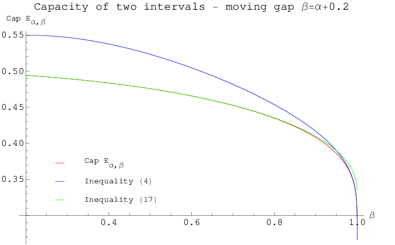
The upper bound of Schiefermayr [17] and our simple upper bound obtained by polarization are given by (4) and (3). The upper bound (9) for $n=2$ reads (recall that $\theta(\alpha)\equiv\arccos(\alpha)$):

$$\mathrm{cap\,}{E}\leq\frac{1}{2}\cos\left([\theta(\beta)-\theta(\alpha)]/2\right).$$

(17)

Figure 2 illustrates these two bounds and the value of capacity computed by (10). Again we have chosen two typical situation - the moving gap and the spreading gap. Since Schiefermayr’s inequality (4) is asympotically precise when one of the intervals vanishes his bound becomes more precise in a narrow neighbourhoods of the right end of the $\alpha$ and $\beta$ ranges. Our bound provides almost uniform and tight fit in the whole parameter ranges.

For $n>2$ our lower bound (7) differs from that of Solynin [19, formula (2.7)]. In particular for $n=3$ [19, formula (2.7)] can be written as

$$\mathrm{cap\,}{E}\geq\frac{1}{2}\max\left(\sin\frac{\pi(\pi-\theta(b_{1}))}{2(\pi-\theta(\delta_{1}))}\right)^{2(\pi-\theta(\delta_{1}))^{2}/\pi^{2}}\left(\sin\frac{\pi(\theta(a_{2})-\theta(\gamma))}{2(\theta(\delta_{1})-\theta(\gamma))}\right)^{2(\theta(\delta_{1})-\theta(\gamma))^{2}/\pi^{2}}\\ \times\left(\sin\frac{\pi(\theta(\gamma)-\theta(b_{2}))}{2(\theta(\gamma)-\theta(\delta_{2}))}\right)^{2(\theta(\gamma)-\theta(\delta_{2}))^{2}/\pi^{2}}\left(\sin\frac{\pi\theta(a_{3})}{2\theta(\delta_{2})}\right)^{2\theta(\delta_{2})^{2}/\pi^{2}},$$

(18)

where the maximum is taken over $\delta_{1}\in(b_{1},a_{2})$, $\gamma\in(a_{2},b_{2})$ and $\delta_{2}\in(b_{2},a_{3})$, while the bound (7) takes the form

$$\mathrm{cap\,}{E}\geq\frac{1}{2}\max\left(\frac{1}{2}\left[1+\cos\frac{\pi(\theta(b_{1})-\theta(\delta_{1}))}{\pi-\theta(\delta_{1})}\right]\right)^{(\pi-\theta(\delta_{1}))^{2}/\pi^{2}}\\ \times\left(\frac{1}{2}\left[\cos\frac{\pi(\theta(b_{2})-\theta(\delta_{2}))}{\theta(\delta_{1})-\theta(\delta_{2})}-\cos\frac{\pi(\theta(a_{2})-\theta(\delta_{2}))}{\theta(\delta_{1})-\theta(\delta_{2})}\right]\right)^{(\theta(\delta_{1})-\theta(\delta_{2}))^{2}/\pi^{2}}\left(\frac{1}{2}\left[1-\cos\frac{\pi\theta(a_{3})}{\theta(\delta_{2})}\right]\right)^{\theta(\delta_{2})^{2}/\pi^{2}},$$

(19)

where the maximum is taken over $\delta_{1}\in(b_{1},a_{2})$ and $\delta_{2}\in(b_{2},a_{3})$. It can be seen from the proof of [19, formula (2.7)] that for any choice of $\gamma$ the latter estimate is greater (i.e. better) than the former if $\delta_{i}$, $i=1,2$, take the same values in both formulas. Similar statement holds for $n>3$.

The upper bound (9) for $n=3$ reads

$$\mathrm{cap\,}{E}\leq\frac{1}{2}\left\{\cos\left([\theta(a_{2})-\theta(b_{1})+\theta(a_{3})-\theta(b_{2})]/2\right)\right\}^{1/2}.$$

(20)

We compare all three bounds with each other and the value of capacity computed by (16) on Figure 3. Again we have chosen a spreading gap as one typical situation while as the other typical situation we have taken two simultaneously moving gaps. The figure confirms our prediction that that bound (19) is more precise than (18) in both situation.

This work supported by Far Eastern Branch of the Russian Academy of Sciences (grants 09-III-A-01-008 and 09-II-CO-01-003), Russian Basic Research Fund (grant 08-01-00028-a) and the Presidential Grant for Leading Scientific Schools (grant 2810.2008.1).

References

- [1] N.I. Achieser, Über einige Funktionen, welche in zwei gegebenen Intervallen am weginsten von Null abweichen, I. Teil, Bulletin de Academie des Sciences de L’URSS, 1932, 1163–1202.
- [2] N.I. Achieser, Über einige Funktionen, welche in zwei gegebenen Intervallen am weginsten von Null abweichen, II. Teil, Bulletin de Academie des Sciences de L’URSS, 1933, 309–344.
- [3] H. Alzer and S.-L. Qui, Monotonicity theorems and inequalities for complete elliptic integrals, Journal of Comp. and Appl. Math., 172, 2004, 289–312.
- [4] G.D. Anderson, M.K. Vamanamurthy and M. Vourinen, Functional inequalities for complete elliptic integrals and their ratios, SIAM J. Math. Anal. 21, no.2 (1990), 536–549.
- [5] V.V. Andrievskii, On the Green function for a complement of a finite number of real intervals. Constr. Approx., 20 (2004), 4, 565–583.
- [6] L.V. Ahlfors, Conformal invariants. Topics in geometric function theory, New York, McGrow-Hill Book Co., 1973.
- [7] V.N. Dubinin, Symmetrization in the geometric theory of functions of a complex variable. Russ. Math. Surv. vol.49, no.1, 1–79 (1994); translation from Usp. Mat. Nauk 49, No.1(295), 3–76 (1994).
- [8] V.N. Dubinin and D. Karp, Capacities of certain plane condensers and sets under simple geometric transformations, Complex Variables and Elliptic Equations, vol.53, no. 6 (2008), 607–622, http://dx.doi.org/10.1080/17476930701734292
- [9] M. Ebree, L.N. Trefethen, Green’s functions for multiply connected domains via conformal mapping, SIAM Review, vol.41, no. 4 (1999), 745–761.
- [10] T. Falliero, A. Sebbar, Capacité de la réunion de troi intervalles et function thta de genre 2, C.R. Acad.Sci. Paris, 328, Série I, 763–766, 1999.
- [11] T. Falliero and A. Sebbar, Capacite de la reunion de trois intervalles et fonctions theta de genre 2. J. Math. Pures Appl. (9) 80 (2001), 4, 409–443.
- [12] J. Gillis, Tchebycheff polynomials and the transifinite diameter, American Journal of Mathematics, 63, 1941, 283–290.
- [13] G.M. Goluzin, Geometric theory of functions of a complex variable, Providence, R. I.:American Mathematical Society (AMS), VI, 1969.
- [14] K. Haliste, On extremal configuration for capacity, Arkiv for Mat., vol.27, no.1, 1989, 97–104.
- [15] S. Kirsch, Transfinite diameter, Chebyshev Constant and Capacity, Handbook of Complex Ananlysis: Geometric Function Theory, Volume 2, ed. by R. Kühnau, Elsevier, 2005.
- [16] R.M. Robinson, On the transifinite diameters of some related sets, Mathematische Zeitschrift, 108, 1969, 377–380.
- [17] K. Schiefermayr, An upper bound for the logarithmic capacity of two intervals, Complex Variables and Elliptic Equations, vol.53, no.1(2008), 65–75.
- [18] J. Shen, G. Strang and A.J. Wathen, The potential theory of several intervals and its applications. Appl. Math. Optim. vol.44, no. 1(2001), 67–85.
- [19] A.Yu. Solynin, Extremal configurations in some problems of capacity and harmonic measure, Journal of Mathematical Sciences, 89, 1998, 1031–1049.
- [20] V. Totik, Metric properties of harmonic measure, Memoirs of AMS, vol.184 (2006), no.867.
- [21] H. Widom, Extremal polynomials associated with a system of curves in the complex plane, Adv. in Math., 3, 127–232.