Surfactant-induced migration of a spherical drop in Stokes flow

James A. Hanna and Petia M. Vlahovska Affiliation: Thayer School of Engineering, Dartmouth College, 8000 Cummings Hall, Hanover, NH 03755, USA

August 24, 2026

Abstract

In Stokes flows, symmetry considerations dictate that a neutrally-buoyant spherical particle will not migrate laterally with respect to the local flow direction. We show that a loss of symmetry due to flow-induced surfactant redistribution leads to cross-stream drift of a spherical drop in Poiseuille flow. We derive analytical expressions for the migration velocity in the limit of small non-uniformities in the surfactant distribution, corresponding to weak-flow conditions or a high-viscosity drop. The analysis predicts migration towards the flow centerline.

pacs

47.15.G-, 47.55.Dk, 47.57.Bc

I Introduction

In his pioneering studies of blood flow, Poiseuille observed the motion of cells away from the walls of small vessels [1]. This phenomenon proved to be a universal feature of particulate flows in tubes, and the mechanisms leading to particle motion transverse to the flow direction have since attracted considerable research effort [2].

A classic result in microhydrodynamics is that lateral migration of a neutrally-buoyant, non-deformable spherical particle is prohibited in the creeping-flow limit, where viscosity dampens fluid acceleration and inertial effects are negligible. The result arises from the linearity of the Stokes equations and boundary conditions, and the symmetry of the problem under flow-reversal [3, 4]. However, such cross-stream drift may occur if the symmetry is lost, e.g. by particle deformation in a shear gradient or in the presence of a wall [2]. A small-deformation solution for a drop with a clean (surfactant-free) interface predicts lateral motion in unbounded Poiseuille flow, with the direction of motion depending on the ratio of drop and suspending fluid viscosities [5]. In this note, we investigate the possibility of cross-stream migration of a non-deforming spherical drop, induced by asymmetric interfacial tension resulting from redistribution of a surfactant.

II Problem formulation

Let us consider a drop with radius $a$ and viscosity ${\lambda}\eta$ , embedded in an ambient fluid with viscosity $\eta$ . A surfactant, insoluble in the bulk phases, is adsorbed on the drop interface; diffusion of surfactant is neglected. The average surfactant concentration is $\Gamma_{\mathrm{eq}}$ , the corresponding interfacial tension is $\sigma_{\mathrm{eq}}$ , and $\sigma_{0}$ is the interfacial tension in the absence of surfactant. The drop is placed in an unbounded plane Poiseuille flow ${\bf v}^{\infty}=\left(U^{\prime}-\alpha y^{\prime 2}\right)\bm{\mathrm{\hat{x}}},$ where $\alpha$ is a measure of the curvature of the flow profile, $\bm{\mathrm{\hat{x}}}$ is the unit-vector in the flow direction, and $U^{\prime}\bm{\mathrm{\hat{x}}}$ is the velocity at the centerline. If the initial drop position is at a distance $y_{0}$ off-center, the drop “sees” a combination of quadratic, linear shear, and uniform flows. In a coordinate system centered on, and translating with, the drop, the flow becomes

{\bf v}^{\infty}=\left(-\dot{\gamma}y-\alpha y^{2}\right)\bm{\mathrm{\hat{x}}}-{\bf U}_{\mathrm{mig}}\,,

(1)

where $\dot{\gamma}=2\alpha y_{0}$ is the local shear rate, and the migration velocity ${\bf U}_{{\mathrm{mig}}}$ is the difference between the velocities of the drop and the undisturbed flow at the drop center.

Refer to caption — Figure 1: An illustration of the problem. A drop is placed in unbounded Poiseuille flow at a distance $y_{0}$ from the flow centerline.

In creeping flows, a drop remains spherical provided that the capillary number is small

\mbox{\it Ca}=\frac{\eta\alpha a^{2}}{\sigma_{\mathrm{eq}}}\ll 1\,,

(2)

where the velocity scale is $U_{c}=\alpha a^{2}$ . Convection by the surrounding flow creates non-uniformities in the surfactant distribution. The ratio of surfactant relaxation and convection time scales defines the inverse Marangoni number

\mbox{\it Ma}^{-1}=\frac{\eta\alpha a^{2}}{\Delta\sigma}\;,\;\Delta\sigma\!=\!\sigma_{0}\!-\!\sigma_{\mathrm{eq}}\,,

(3)

which can also be viewed as the ratio of viscous stresses to the characteristic Marangoni stresses (gradients in surface tension). For a dilute surfactant monolayer, a linear “perfect gas” interfacial equation of state relates surface tension and local surfactant concentration: $\sigma(\Gamma)-\sigma_{\mathrm{eq}}=\mbox{\it Ma}\left(1-\Gamma/\Gamma_{\mathrm{eq}}\right)$ . Henceforward, all quantities are normalized using $a$ , $\eta$ , $U_{c}$ , and $\Gamma_{\mathrm{eq}}$ .

The flow is described by the Stokes equations. The velocity and pressure fields ${\bf v}$ and $p$ satisfy

\begin{split}\nabla p&=\nabla^{2}{\bf v}\quad,\quad\nabla\cdot{\bf v}=0\quad\mathrm{outside}\,,\\ \nabla p&=\lambda\nabla^{2}{\bf v}\quad,\quad\nabla\cdot{\bf v}=0\quad\mathrm{inside}\,,\end{split}

(4)

and ${\bf v}$ is continuous everywhere. The viscous shearing stresses at the interface are balanced by Marangoni stresses $\nabla_{s}\sigma=-\mbox{\it Ma}\nabla_{s}\Gamma$ . To close the problem, we need an evolution equation for the surfactant. This is supplied by a conservation equation for bulk-insoluble, non-diffusing surfactant on a moving interface:

\frac{\partial\Gamma}{\partial t}+\nabla_{s}\cdot({\bf v}_{s}\Gamma)+\Gamma({\bf v}\cdot\bm{\mathrm{\hat{n}}})\nabla\cdot\bm{\mathrm{\hat{n}}}=0\,,

(5)

where ${\bf v}_{s}$ is the velocity component tangential to the surface. For a sphere, the mean curvature $\nabla\cdot\bm{\mathrm{\hat{n}}}=2$ .

III Solution

By the linearity of the Stokes equations, the perturbation in the imposed Poiseuille flow around the surfactant-covered drop may be given as a superposition of two components. The first is a flow about a clean, surfactant–free drop placed in the Poiseuille flow. The second is a flow driven by Marangoni stresses arising from non-uniform surfactant coverage of a drop in a quiescent fluid [6]. In similar fashion, the drop migration may be decomposed into

{\bf U}_{{\mathrm{mig}}}={\bf U}^{0}_{{\mathrm{mig}}}+{\bf U}^{s}_{{\mathrm{mig}}}(\Gamma)\,.

(6)

The velocity perturbation due to a clean spherical drop gives rise to slip, but no lateral migration [7]:

{\bf U}^{0}_{{\mathrm{mig}}}=-\frac{\lambda}{3\lambda+2}\bm{\mathrm{\hat{x}}}\,.

(7)

Note that ${\bf U}^{0}_{{\mathrm{mig}}}$ is normalized by $\alpha a^{2}$ , so the dimensional slip velocity depends on the flow curvature. To determine the surfactant contribution ${\bf U}^{s}_{{\mathrm{mig}}}$ , we solve for the velocity field about the surfactant-covered drop using the formalism developed by Bławzdziewicz et al. [6]. In the original work, the method was applied to the dynamics of a stationary surfactant-covered drop in a linear flow. We have generalized the approach to treat a translating drop in higher-order flows. Owing to the spherical symmetry of the problem, all quantities are represented in terms of spherical harmonics (see Appendix A for definitions). Accordingly, the surfactant concentration $\Gamma$ is expanded in scalar harmonics (26)

\Gamma=1+\sum_{j=1}^{\infty}\sum_{m=-j}^{j}g_{jm}Y_{jm}\left(\theta,\varphi\right)\,,

(8)

where $\theta,\,\varphi$ denote the spherical coordinate angles. The velocity field is expanded in a set of fundamental solutions of the Stokes equations (27) and (28) [8, 6]

\begin{split}{\bf v}_{{\mathrm{out}}}=&\;c^{\infty}_{jmq}\left[{\bf u}^{+}_{jmq}({\bf r})-{\bf u}^{-}_{jmq}({\bf r})\right]+c_{jmq}{\bf u}^{-}_{jmq}({\bf r})\,,\\ {\bf v}_{{\mathrm{in}}}=&\;c_{jmq}{\bf u}^{+}_{jmq}({\bf r})\,.\\ \end{split}

(9)

Summation over repeated indices is implied. The functions ${\bf u}^{\pm}_{jmq}$ are vector solid harmonics related to the harmonics in the Lamb solution. With respect to a sphere, ${\bf u}^{\pm}_{jm2}$ is radial, while ${\bf u}^{\pm}_{jm0}$ and ${\bf u}^{\pm}_{jm1}$ are tangential; ${\bf u}^{\pm}_{jm1}$ is surface-solenoidal ( $\nabla_{s}\cdot{\bf u}^{\pm}_{jm1}=0$ ). The far-field (imposed) flow is specified by ${\bf v}^{\infty}\!=\!c^{\infty}_{jmq}{\bf u}^{+}_{jmq}$ ; coefficients for the Poiseuille flow (1) are listed in Appendix B. The velocity fields defined in (9) are naturally continuous across the interface because the basis fields ${\bf u}^{\pm}_{jmq}$ reduce to the corresponding vector spherical harmonics ${\bf y}_{jmq}$ at $r\!=\!1$ . The velocity coefficients $c_{jmq}$ are determined from the stress balance equations listed in Appendix C. A fixed spherical shape limits the normal surface velocity to rigid body translation. Thus, for $j\!>\!1$ , $c_{jm2}\!=\!0$ , and the other two coefficients $c_{jmq}$ are determined from the tangential stress balances alone, as use of the normal stress balance in conjunction with shape specification over-constrains the problem. However, both the tangential and normal stress balances are used to determine the $c_{1mq}$ , which correspond to translational and rotational motions of the drop.

The velocity coefficients are decomposed into clean-drop and surfactant contributions: $c_{jmq}\!=\!c^{0}_{jmq}+c^{s}_{jmq}(\Gamma)$ . We obtain for the surfactant-driven flow

\begin{split}c^{s}_{jm0}=&-\frac{\delta_{1j}}{(3{\lambda}+2)}\,\frac{\sqrt{2}}{\;3}\mbox{\it Ma}\,g_{jm}\\ &-\frac{(1-\delta_{1j})}{{\lambda}+1}\frac{\sqrt{j(j+1)}}{(2j+1)}\mbox{\it Ma}\,g_{jm}\,,\\ c^{s}_{jm1}=&\;\,0\,,\\ c^{s}_{jm2}=&\quad\,\frac{\delta_{1j}}{(3{\lambda}+2)}\,\frac{2}{3}\mbox{\it Ma}\,g_{jm}\,,\end{split}

(10)

where $\delta_{kl}$ is the Kronecker delta. The solution for $j\!>\!1$ is identical to that of Bławzdziewicz et al. [6]. The clean-drop flow is

\begin{split}c^{0}_{jm0}=&\,\frac{\delta_{1j}}{3{\lambda}+2}\left[(2{\lambda}+3)c^{\infty}_{jm0}+\sqrt{2}({\lambda}-1)c^{\infty}_{jm2}\right]\\ +&\frac{1-\delta_{1j}}{{\lambda}+1}\left[2c^{\infty}_{jm0}-\frac{3}{\sqrt{j(j+1)}}c^{\infty}_{jm2}\right]\,,\\ c^{0}_{jm1}=&\,\frac{2j+1}{2+j+{\lambda}(j-1)}c^{\infty}_{jm1}\,,\\ c^{0}_{jm2}=&\,\frac{\delta_{1j}}{3{\lambda}+2}\left[\sqrt{2}({\lambda}-1)c^{\infty}_{jm0}+({\lambda}+4)c^{\infty}_{jm2}\right]\,.\end{split}

(11)

The drop migration velocity is the difference between the volume-averaged velocity of the drop and the undisturbed velocity at the drop center

{\bf U}_{{\mathrm{mig}}}=-{\bf v}^{\infty}(0)+\frac{3}{4\pi}\int_{drop}{\bf v}({\bf r}){\mathrm{d}}{\bf r}\,.

(12)

For a spherical drop, only the ${\bf u}^{+}_{1m2}$ contribute to the integral. Hence we obtain

\begin{split}{\bf U}_{{\mathrm{mig}}}=\textstyle{\sqrt{\frac{3}{8\pi}}}&\left[-(c_{112}-c_{1-12})\bm{\mathrm{\hat{x}}}\right.\\ &\left.-{\mathrm{i}}(c_{112}+c_{1-12})\bm{\mathrm{\hat{y}}}+\textstyle{\sqrt{2}}\,c_{102}\bm{\mathrm{\hat{z}}}\right]\,.\end{split}

(13)

The above expression, in conjunction with (11) and (30), yields the slip term (7). Using (10) instead of (11) yields the surfactant-induced migration

\begin{split}{\bf U}_{{\mathrm{mig}}}^{s}=\textstyle{\frac{\mbox{\it Ma}}{\sqrt{6\pi}(3\lambda+2)}}&\left[-(g_{11}-g_{1-1})\bm{\mathrm{\hat{x}}}\right.\\ &\left.-{\mathrm{i}}(g_{11}+g_{1-1})\bm{\mathrm{\hat{y}}}+\textstyle{\sqrt{2}}\,g_{10}\bm{\mathrm{\hat{z}}}\right]\,.\end{split}

(14)

The surfactant distribution coefficients $g_{1m}$ are determined from the evolution equation [6, 9]

\begin{split}\frac{\partial g_{jm}}{\partial t}&=C_{jm}+\left[\Omega_{jmj_{2}m_{2}}+\Lambda_{jmj_{2}m_{2}}\right]g_{j_{2}m_{2}}\\ &+\mbox{\it Ma}\left[W(j)g_{jm}+\Theta_{jmj_{1}m_{1}j_{2}m_{2}}g_{j_{2}m_{2}}g_{j_{1}m_{1}}\right]\,.\end{split}

(15)

The terms in this equation are defined in Appendix D. The first three terms describe convection of surfactant by the imposed flow: $\Omega$ describes rotation by the linear shear component of the flow, while $C_{jm}$ and $\Lambda$ describe redistribution by other components of the flow. The terms proportional to Ma pertain to flows driven by Marangoni stresses. The linear term describes relaxation towards the equilibrium uniform surfactant distribution, while the quadratic term describes convection of surfactant by the surfactant-induced flow.

The migration velocity of a spherical drop is related to the $j\!=\!1$ modes of the surfactant distribution (14). Equation (15) shows that these modes can be created by several interactions between velocity and surfactant field components, e.g. quadratic flow ( $j\!=\!3$ ) coupling to sheared surfactant ( $j\!=\!2$ ).

For arbitrary distortions of the surfactant concentration, equation (15) must be integrated numerically to determine $g_{1m}$ and ${\bf U}_{\mathrm{mig}}$ . Analytical solutions are possible if we consider quasi-steady, slightly-perturbed surfactant distributions. Quasi-steady implies that the surfactant evolution occurs on a faster time scale than the drop migration, i.e. $\eta a/\Delta\sigma\ll{a}/{U_{\mathrm{mig}}}$ . Small disturbances in the surfactant concentration admit a solution in the form of a regular perturbation expansion

{\bf U}_{\mathrm{mig}}={\bf U}_{\mathrm{mig}}^{(0)}+{\bf U}^{(1)}_{\mathrm{mig}}+\ldots

(16)

The choice of small parameter depends on the flow regime of interest. In weak flows, surfactant relaxation towards the equilibrium distribution is fast, and $\mbox{\it Ma}^{-1}$ is the relevant small parameter, being the ratio of the time scales associated with Marangoni relaxation and distortion by convection. If the drop is far away from the centerline ( $y_{0}\!\gg\!1\,$ ), the shear flow $2\alpha y_{0}y\,$ is dominant over the quadratic flow $\alpha y^{2}$ . The extensional part of the shear convects surfactant towards two poles on the drop that correspond to the straining axis of the flow. Concurrently, the rotational component of the shear rotates the drop, limiting these distortions. The ratio of rotational and extensional time scales [9] is $\sim\!{\lambda}^{-1}$ , so this is an appropriate small parameter for very viscous drops. Next, we examine these two regimes in more detail.

IV Results and Discussion

IV.1 Weak flow / Nearly-incompressible surfactant: $Ma^{-1}\ll 1$ and ${\lambda}=O(1)$

In this regime, only Marangoni stresses oppose the convection of surfactant. If $\mbox{\it Ma}^{-1}\ll 1$ , following the discussion in Bławzdziewicz et al. [6], we introduce a regular expansion for the surfactant concentration: $g_{jm}=\sum_{k=0}^{\infty}\mbox{\it Ma}^{-k-1}g_{jm}^{(k)}\,$ . At leading order, the evolution equation (15) becomes $0=C_{jm}+{W(j)}{g}^{(0)}_{jm}$ . Solving for ${g}^{(0)}_{jm}$ yields

	$\displaystyle{g}^{(0)}_{1m}$	$\displaystyle=$	$\displaystyle\frac{5}{\sqrt{2}}\left(c^{\infty}_{1m0}-\sqrt{2}\,c^{\infty}_{1m2}\right)\quad\mbox{and}$		(17)
	$\displaystyle g^{(0)}_{jm}$	$\displaystyle=$	$\displaystyle\frac{2j+1}{j(j+1)}\left[2\sqrt{j(j+1)}c^{\infty}_{jm0}-3c^{\infty}_{jm2}\right]\,\mbox{for}\,\,j>1\,.$

Inserting the ${g}^{(0)}_{1m}$ expression in (14) and (6) gives

{\bf U}^{(0)}_{{\mathrm{mig}}}=-\frac{1}{3}\bm{\mathrm{\hat{x}}}\,.

(18)

Thus, at leading order, the Marangoni stresses immobilize the interface. The surface flow is incompressible, and the drop behaves like a rigid sphere.

At next order, the evolution equation is

\begin{split}0=&\left[\Omega_{jmj_{2}m_{2}}+\Lambda_{jmj_{2}m_{2}}\right]{g}^{(0)}_{j_{2}m_{2}}+{W(j)}{g}^{(1)}_{jm}\,\\ &+\Theta_{jmj_{1}m_{1}j_{2}m_{2}}{g}^{(0)}_{j_{1}m_{1}}{g}^{(0)}_{j_{2}m_{2}}\,,\end{split}

(19)

and the ${g}^{(1)}_{1m}$ give rise to a cross-stream migration velocity

\begin{split}{\bf U}^{(1)}_{{\mathrm{mig}}}&=-\mbox{\it Ma}^{-1}{y_{0}}\frac{3\lambda+17}{9(\lambda+4)}\,\bm{\mathrm{\hat{y}}}\,.\\ \end{split}

(20)

Note that the dimensional cross-stream velocity is quadratic in $\alpha$ . Hence, its direction does not change upon reversal of the flow direction. Its magnitude depends linearly on $y_{0}$ , the distance from the centerline, and thus monotonically on the local shear rate, $\sim\alpha y_{0}$ . It is directed towards the centerline or, equivalently, towards lower shear rates, for all values of the viscosity ratio ${\lambda}$ .

IV.2 Far from the centerline / High viscosity drops: ${\lambda}^{-1}\ll 1$ and $\mbox{\it Ma}=O(\lambda)$

In this regime, both rotation and Marangoni relaxation limit convective distortions of the surfactant distribution. If ${\lambda}^{-1}\ll 1$ , we expand $g_{jm}=\sum_{k=0}^{\infty}{\lambda}^{-k-1}g_{jm}^{(k)}$ and introduce $\tilde{\mbox{\it Ma}}\equiv{\lambda}^{-1}{\mbox{\it Ma}}$ . The leading order equation for the surfactant distribution is the $\lambda\!\rightarrow\!\infty$ limit of (15). Only the first convection term, the linear Marangoni term, and the rigid rotation within the $\Omega$ term survive. Thus,

\begin{split}0=\tilde{C}_{jm}+\Omega_{jmjm}{g}^{(0)}_{jm}+\tilde{\mbox{\it Ma}}\,\tilde{W}(j){g}^{(0)}_{jm}\,,\end{split}

(21)

where ${C}(jm)\equiv\lambda^{-1}\tilde{C}(jm)$ and ${W}(j)\equiv\lambda^{-1}\tilde{W}(j)$ as $\lambda\!\rightarrow\!\infty$ . Solving for $g_{1m}^{(0)}$ yields

g_{10}^{(0)}=0\quad,\quad g_{1\pm 1}^{(0)}=\frac{2}{\mp 2\tilde{\mbox{\it Ma}}+3{\mathrm{i}}y_{0}}\sqrt{\frac{2\pi}{3}}\,.

(22)

Inserting in (14) and (6) and keeping terms up to order $\lambda^{-1}$ gives a slip velocity

U^{x}_{{\mathrm{mig}}}=-\frac{1}{3}+\frac{2}{9{\lambda}}-\frac{8}{9{\lambda}}\frac{\tilde{\mbox{\it Ma}}^{2}}{9y_{0}^{2}+4\tilde{\mbox{\it Ma}}^{2}}\quad,

(23)

and a cross-stream drift

U^{y}_{{\mathrm{mig}}}=-\frac{4}{3{\lambda}}\frac{y_{0}\tilde{\mbox{\it Ma}}}{9y_{0}^{2}+4\tilde{\mbox{\it Ma}}^{2}}\quad.

(24)

As before, reversing the flow direction changes the sign of the slip velocity but leaves the cross-stream velocity unaffected. As $\tilde{\mbox{\it Ma}}\rightarrow\infty$ , $\lambda\rightarrow\infty$ , or $y_{0}\rightarrow 0$ , rigid sphere behavior is recovered; cross-stream motion vanishes, and the slip is given by the Faxén result (18). While the cross-stream velocity is always directed towards the centerline, its magnitude is a non-monotonic function of position, with maxima at $y_{0}=\pm\frac{2}{3}{\tilde{\mbox{\it Ma}}}$ .

IV.3 Arbitrary perturbation in the surfactant distribution

The present analysis is easily extended to larger redistributions and the general surfactant dynamics of the full equation (15). A drop trajectory $y_{0}(t)$ is determined by numerical solution of this equation to obtain $dy_{0}/dt=U^{y}_{{\mathrm{mig}}}\left[y_{0},\Gamma(y_{0})\right]$ . The evolution equation for the surfactant distribution was truncated at $j\!=\!6$ ; this was enough to produce convergent results.

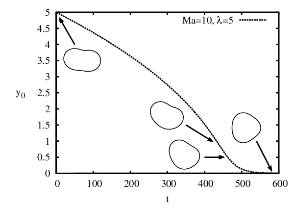
A typical drop trajectory is shown in Figure 2, along with shapes representing the distribution of surfactant in the $xy$ plane for the high viscosity expansion at several distances from the centerline. Figure 3 shows three such distributions as a function of the azimuthal angle $\varphi$ . The distribution is three-lobed near the centerline and two-lobed far from the centerline. These shapes reflect the dominance of the quadratic ( $j\!=\!3$ ) and linear shear ( $j\!=\!2$ ) components of the flow at these respective locations. The behavior of the particle is governed by rotation in the high-shear-rate region far from the centerline, and by Marangoni effects near the centerline.

The $g_{1m}$ are linear gradients in surfactant concentration; migration towards the centerline results from an excess of surfactant on the drop hemisphere facing the centerline. At the centerline, $g(\varphi)\!=\!g(-\varphi)$ and $U^{y}_{{\mathrm{mig}}}$ vanishes. This symmetry is also approached as $y_{0}\rightarrow\infty$ in the unbounded flow. Thus, $U^{y}_{{\mathrm{mig}}}$ has an extremum, and the trajectory an inflection point. This point is a rough indicator of the distance from the centerline, of order $\frac{\mbox{\it Ma}}{\lambda}$ , beyond which the large Marangoni expansion is inadequate even as a qualitative descriptor of the drop’s behavior. The high viscosity expansion captures the qualitative behavior of quasi-steady trajectories at all distances. Figures 4 and 5 show the cross-stream migration velocity as a function of distance from the centerline for several values of the parameters, along with the two expansions.

The numerical results suggest that cross-stream migration of a surfactant-covered spherical drop is directed towards an equilibrium position at the flow centerline. This result agrees with those found for other particles, such as capsules [10] and vesicles [11], whose interfaces are governed by Marangoni-like stresses, and with simulations of surfactant-covered, deformable, equi-viscous drops [12].

However, a quasi-steady treatment of the drop dynamics is not always appropriate, and more complicated non-monotonic trajectories are possible. We note one interesting feature that occurs when $\frac{\mbox{\it Ma}}{\lambda}$ is small and the drop experiences its greatest cross-stream velocity very close to the centerline. In such cases, the drop may overshoot and execute small-amplitude damped oscillations around the centerline, as shown in Figure 6. Similar behavior has been predicted for vesicles [11].

We may consider a linearized dynamics for a viscous drop near the centerline by noting that $\dot{y}_{0}\sim-\frac{\mbox{\it Ma}}{\lambda}(g_{11}+g_{1-1})$ according to (14). The damping term is provided by the linear relaxation term of (15), which $\sim-\frac{\mbox{\it Ma}}{\lambda}$ . Finally, either (20) or (24) indicates that when $\ddot{y}_{0}\rightarrow 0$ and $y_{0}\ll 1$ , $\dot{y}_{0}\sim-\frac{1}{\mbox{\it Ma}}y_{0}$ . Hence, denoting unknown constants as $k_{i}$ ,

\ddot{y}_{0}+k_{1}\frac{\mbox{\it Ma}}{\lambda}\dot{y}_{0}+k_{2}\frac{1}{\lambda}y_{0}=0\,.

(25)

Such an oscillator will be critically damped when $\mbox{\it Ma}=k_{3}\sqrt{\lambda}$ ; this prediction is supported by the numerical results shown in Figure 7.

V Conclusions

We have shown that the presence of small amounts of surfactant can significantly affect drop motions in quadratic flows. In contrast with a clean, deformable drop [5], for which the direction of migration depends on viscosity ratio, a surfactant-covered spherical drop always migrates towards the flow centerline.

VI Acknowledgments

This work was supported in part by NSF CAREER award CBET–0846247. Acknowledgment is made to the Donors of the American Chemical Society Petroleum Research Fund for partial support of this research.

Appendix A Harmonics and velocity fields

Scalar and vector spherical harmonics are defined as

\begin{split}Y_{jm}(\theta,\varphi)&=\textstyle\left[\frac{2j+1}{4\pi}\frac{(j-m)!}{(j+m)!}\right]^{\frac{1}{2}}(-1)^{m}P_{j}^{m}(\cos\theta)e^{{\rm i}m\varphi}\,,\\ &{\bf y}_{jm0}=\left[j\left(j+1\right)\right]^{-\frac{1}{2}}r\,\nabla_{\Omega}Y_{jm}\,,\\ &{\bf y}_{jm1}=-{\mathrm{i}}\bm{\mathrm{\hat{r}}}\times{\bf y}_{jm0}\,,\\ &{\bf y}_{jm2}=\bm{\mathrm{\hat{r}}}\,Y_{jm}\,,\\ \end{split}

(26)

where the $P_{j}^{m}$ are the Legendre polynomials, and $\nabla_{\Omega}$ is the angular part of the gradient operator. The velocity basis functions are


$\displaystyle{\bf u}^{-}_{jm0}$	$\displaystyle={\textstyle\frac{1}{2}}r^{-j}\left(2-j+jr^{-2}\right){\bf y}_{jm0}$
	$\displaystyle+{\textstyle\frac{1}{2}}r^{-j}\left[j\left(j+1\right)\right]^{\frac{1}{2}}\left(1-r^{-2}\right){\bf y}_{jm2}\,,$	(27a)
$\displaystyle{\bf u}^{-}_{jm1}$	$\displaystyle=\textstyle r^{(-j-1)}{\bf y}_{jm1}\,,$	(27b)
$\displaystyle{\bf u}^{-}_{jm2}$	$\displaystyle={\textstyle\frac{1}{2}}r^{-j}\left(2-j\right)(\textstyle\frac{j}{j+1})^{\frac{1}{2}}\left(1-r^{-2}\right){\bf y}_{jm0}$
	$\displaystyle+{\textstyle\frac{1}{2}}r^{-j}\left(j+(2-j)r^{-2}\right){\bf y}_{jm2}\,,$	(27c)


$\displaystyle{\bf u}^{+}_{jm0}$	$\displaystyle={\textstyle\frac{1}{2}}r^{j-1}\left(-(j+1)+(j+3)r^{2}\right){\bf y}_{jm0}$
	$\displaystyle-{\textstyle\frac{1}{2}}r^{j-1}\left[j\left(j+1\right)\right]^{\frac{1}{2}}\left(1-r^{2}\right){\bf y}_{jm2}\,,$	(28a)
$\displaystyle{\bf u}^{+}_{jm1}$	$\displaystyle=\textstyle r^{j}{\bf y}_{jm1}\,,$	(28b)
$\displaystyle{\bf u}^{+}_{jm2}$	$\displaystyle={\textstyle\frac{1}{2}}r^{j-1}\left(3+j\right)(\textstyle\frac{j+1}{j})^{\frac{1}{2}}\left(1-r^{2}\right){\bf y}_{jm0}$
	$\displaystyle+{\textstyle\frac{1}{2}}r^{j-1}\left(j+3-(j+1)r^{2}\right){\bf y}_{jm2}\,.$	(28c)

Appendix B Imposed flow

The unbounded plane Poiseuille flow (1) seen by a migrating particle is represented as

{\bf v}^{\infty}=c_{jmq}^{\infty}{\bf u}^{+}_{jmq}\,,

(29)

with coefficients

\begin{split}\textstyle&c^{\infty}_{3\pm 30}=\textstyle\mp\alpha\sqrt{\frac{4\pi}{105}}\,,\quad\;c^{\infty}_{3\pm 32}=\mp\alpha\sqrt{\frac{\pi}{35}}\,,\\ \textstyle&c^{\infty}_{3\pm 10}=\textstyle\mp\alpha\frac{2}{15}\sqrt{\frac{\pi}{7}}\,,\quad c^{\infty}_{3\pm 12}=\mp\alpha\frac{1}{5}\sqrt{\frac{\pi}{21}}\,,\\ \textstyle&c^{\infty}_{2\pm 20}=\textstyle\pm\dot{\gamma}{\mathrm{i}}\sqrt{\frac{\pi}{5}}\,,\quad\;\;\;c^{\infty}_{2\pm 22}=\pm\dot{\gamma}{\mathrm{i}}\sqrt{\frac{2\pi}{15}}\,,\\ \textstyle&c^{\infty}_{2\pm 11}=\textstyle\alpha\frac{2}{3}\sqrt{\frac{\pi}{5}}\,,\quad\;\,c^{\infty}_{101}=-{\mathrm{i}}\dot{\gamma}\sqrt{\frac{2\pi}{3}}\,,\\ \textstyle&\quad c^{\infty}_{1\pm 10}=\textstyle\pm\left(\alpha\frac{4}{5}+2(U_{{\mathrm{mig}}}^{x}\mp{\mathrm{i}}U_{{\mathrm{mig}}}^{y})\right)\sqrt{\frac{\pi}{3}}\,,\\ \textstyle&\quad c^{\infty}_{1\pm 12}=\textstyle\pm\left(\alpha\frac{1}{5}+(U_{{\mathrm{mig}}}^{x}\mp{\mathrm{i}}U_{{\mathrm{mig}}}^{y})\right)\sqrt{\frac{2\pi}{3}}\,,\\ \textstyle&c^{\infty}_{100}=\textstyle-2U_{{\mathrm{mig}}}^{z}\sqrt{\frac{2\pi}{3}}\,,\quad\;\;c^{\infty}_{102}=-2U_{{\mathrm{mig}}}^{z}\sqrt{\frac{\pi}{3}}\,.\\ \end{split}

(30)

Appendix C Hydrodynamic tractions and stress balances

Neglecting isotropic contributions, the hydrodynamic tractions on a sphere may be expanded in harmonics ${\bf t}_{\mathrm{hyd}}=\tau_{jmq}{\bf y}_{jmq}$ , with

\begin{split}\tau^{\mathrm{out}}_{jmq}&=\textstyle\sum_{q^{\prime}}c^{\infty}_{jmq^{\prime}}\left(T_{q^{\prime}q}^{+}-T_{q^{\prime}q}^{-}\right)+c_{jmq^{\prime}}T_{q^{\prime}q}^{-}\,,\\ \tau^{\mathrm{in}}_{jmq}&={\lambda}\textstyle\sum_{q^{\prime}}c_{jmq^{\prime}}T_{q^{\prime}q}^{+}\,,\end{split}

(31)

where $T^{\pm}_{q^{\prime}q}=T^{\pm}_{qq^{\prime}}$ , $T^{\pm}_{00}=\pm(2j+1)$ , $T^{\pm}_{02}=\mp 3\left(\frac{j+1}{j}\right)^{\pm\frac{1}{2}}$ , $T^{\pm}_{11}=\pm\left(j+\frac{1}{2}\right)-\frac{3}{2}$ , $T^{\pm}_{22}=\pm(2j+1)+\frac{3}{\pm\left(j+\frac{1}{2}\right)-\frac{1}{2}}$ , and $T^{\pm}_{01}=T^{\pm}_{12}=0$ .

The tangential stress boundary conditions are

\begin{split}\tau_{jm0}^{\mathrm{out}}-\tau_{jm0}^{\mathrm{in}}=&\;\mbox{\it Ma}\sqrt{j(j+1)}\,g_{jm}\,,\\ \tau_{jm1}^{\mathrm{out}}-\tau_{jm1}^{\mathrm{in}}=&\;0\,,\end{split}

(32)

where a linear equation of state relating surface tension and local surfactant concentration is assumed. The normal stress balance for a spherical drop requires

\tau_{jm2}^{\mathrm{out}}-\tau_{jm2}^{\mathrm{in}}=-2\mbox{\it Ma}\,g_{jm}

(33)

For $j\!>\!1$ , we set $c_{jm2}\!=\!0$ and do not use the normal stress balance condition.

Appendix D Surfactant evolution equation

The surfactant conservation equation on a moving interface is given by (5). Representing all quantities as harmonics and decomposing the velocity field into clean-drop and surfactant contributions leads to (15). The clean-drop terms are

\begin{split}C_{jm}=&\,\left[j(j+1)\right]^{\frac{1}{2}}c^{0}_{jm0}-2c^{0}_{jm2}\,,\\ \Omega_{jmj_{2}m_{2}}=&\,\left[j(j+1)\right]^{\frac{1}{2}}c^{0}_{j_{1}m_{1}1}\,{\cal{C}}^{01}\,,\\ \Lambda_{jmj_{2}m_{2}}=&\,\left[j(j+1)\right]^{\frac{1}{2}}c^{0}_{j_{1}m_{1}0}\,{\cal{C}}^{00}-2\,c^{0}_{j_{1}m_{1}2}\,{\cal{C}}^{22}\,.\end{split}

(34)

Summation over $j_{1}$ and $m_{1}$ is implied, and the $c^{0}_{jmq}$ coefficients refer to equations (11). Using equations (10) to define the vector $\bar{W}(j)$ by

c^{s}_{jmq}\equiv\bar{W}_{q}(j)\mbox{\it Ma}\,g_{jm}\,,

(35)

the surfactant terms are

	$\displaystyle{W}(j)\!\!$	$\displaystyle=$	$\displaystyle\!\!\left[j(j+1)\right]^{\frac{1}{2}}\bar{W}_{0}(j)-2\,\bar{W}_{2}(j)\,,$		(36)
	$\displaystyle\Theta_{jmj_{1}m_{1}j_{2}m_{2}}\!\!$	$\displaystyle=$	$\displaystyle\!\!\left[j(j+1)\right]^{\frac{1}{2}}\bar{W}_{0}(j_{1})\,{\cal{C}}^{00}-2\,\bar{W}_{2}(j_{1})\,{\cal{C}}^{22}\,.$

The Clebsch-Gordan coupling coefficients ${\cal{C}}$ are

\begin{split}{\cal{C}}^{00}&=\,B\left(\begin{array}[]{ccc}j_{1}&j_{2}&j\\ 0&0&0\end{array}\right)\\ &\times\frac{j_{1}(j_{1}+1)+j(j+1)-j_{2}(j_{2}+1)}{\left[j(j+1)j_{1}(j_{1}+1)\right]^{\frac{1}{2}}}\,,\\ {\cal{C}}^{01}&=\,B\left(\begin{array}[]{ccc}j_{1}&j_{2}&j-1\\ 0&0&0\end{array}\right)\\ &\times\left[\frac{(s+1)(s-2j_{2})(s-2j_{1})(s-2j+1)}{j(j+1)j_{1}(j_{1}+1)}\right]^{\frac{1}{2}}\,,\\ {\cal{C}}^{22}&=\,B\left(\begin{array}[]{ccc}j_{1}&j_{2}&j\\ 0&0&0\end{array}\right)\times 2\,,\\ \end{split}

(37)

where $s=j+j_{1}+j_{2}\,$ ,

\begin{split}B=\;&\frac{(-1)^{m}}{2}\left[\frac{(2j+1)(2j_{1}+1)(2j_{2}+1)}{4\pi}\right]^{\frac{1}{2}}\\ &\times\left(\begin{array}[]{ccc}j_{1}&j_{2}&j\\ m_{1}&m_{2}&-m\end{array}\right)\,,\end{split}

and $\left(\begin{array}[]{ccc}j_{1}&j_{2}&j\\ m_{1}&m_{2}&m\end{array}\right)$ denotes the Wigner 3 $j$ -symbol [13].

References

[1] S. P. Sutera and R. Skalak. The history of Poiseuille’s law. Annu. Rev. Fluid Mech., 25:1–19, 1993.
[2] L. G. Leal. Particle motions in a viscous fluid. Ann. Rev. Fluid Mech, 12:435–476, 1980.
[3] F. P. Bretherton. The motion of rigid particles in a shear flow at low Reynolds number. J. Fluid Mech., 14:284–304, 1962.
[4] L. G. Leal. Advanced transport phenomena. Cambridge University Press, Cambridge, 2007.
[5] P. C.-H. Chan and L. G. Leal. The motion of a deformable drop in a second-order fluid. J. Fluid Mech., 92:131–170, 1979.
[6] J. Bławzdziewicz, P. Vlahovska, and M. Loewenberg. Rheology of a dilute emulsion of surfactant-covered spherical drops. Physica A, 276:50–80, 2000.
[7] A. Nadim and H. A. Stone. The motion of small particles and droplets in quadratic flows. Studies in Appl. Math., 85:53–73, 1991.
[8] B. Cichocki, B. U. Felderhof, and R. Schmitz. Hydrodynamic interactions between two spherical particles. PhysicoChem. Hyd., 10:383–403, 1988.
[9] P. Vlahovska, J. Bławzdziewicz, and M. Loewenberg. Nonlinear rheology of a dilute emulsion of surfactant-covered spherical drops in time-dependent flows. J. Fluid Mech., 463:1–24, 2002.
[10] A. Helmy and D. Barthès-Biesel. Migration of a spherical capsule freely suspended in an unbounded parabolic flow. J. Méc. Theor. Appl., 1:859–880, 1982.
[11] G. Danker, P. M. Vlahovska, and C. Misbah. Vesicles in Poiseuille Flow. Phys. Rev. Lett., 102, 2009.
[12] P. J. A. Janssen, P. D. Anderson. Surfactant-covered drops between parallel plates. Chem. Eng. Res. Des., 86:1388-1396, 2008.
[13] A. R. Edmonds. Angular Momentum in Quantum Mechanics. Princeton University Press, Princeton, 1960.