CP-violating Phases in M-theory and Implications for EDMs
Abstract
We demonstrate that in effective theories arising from a class of fluxless compactifications of M-theory on a manifold with low energy supersymmetry, CP-violating phases do not appear in the soft-breaking Lagrangian except via the Yukawas appearing in the trilinear parameters. Such a mechanism may be present in other string compactifications as well; we describe properties sufficient for this to occur. CP violation is generated via the Yukawas since the soft trilinear matrices are generically not proportional to the Yukawa matrices. Within the framework considered, the estimated theoretical upper bounds for electric dipole moments (EDM) of the electron, neutron and mercury are all within the current experimental limits and could be probed in the near future.
I Introduction
The null measurements of the electric dipole moments (EDMs) of the neutron [1], and recently, heavy atoms like Thallium (205Tl)[2, 3] and Mercury (199Hg) [4, 5], have put very strong constraints on the amount of CP violation from new physics beyond the Standard Model (SM). The precision of these measurements is expected to significantly improve in a few years. If an excess above the SM prediction is observed, it requires the presence of new physics beyond the SM. However, since the EDMs, even if observed, are already “small”, this strongly suggests that the new physics must be such that it has an underlying mechanism to naturally suppress EDMs.
In general versions of supersymmetric extensions of the Standard Model, new sources of CP violation can arise from complex phases of the soft supersymmetry breaking parameters. These phases are therefore tightly constrained to be small [6, 7](or to have cancellation [8, 9, 10, 11]) for TeV scale superpartners. Thus, from a theoretical perspective, the existence of such small phases has to be explained by some underlying mechanism. Many studies of supersymmetric models from a low-energy phenomenological perspective focus on the mediation mechanism and only parameterize the supersymmetry breaking. Explaining small soft CP-violating phases, which requires a dynamical understanding of supersymmetry breaking, is especially challenging as this is not available in such a framework. Without a specification of the supersymmetry breaking mechanism, this problem exists in both gravity and gauge-mediated models of supersymmetry breaking in general.
Put differently, whenever supersymmetry is treated as a general TeV-scale effective theory both the values and phases of the soft-breaking masses are treated as arbitrary, and EDMs are typically much larger than experimental values. Many people have argued that such large EDMs are implied or required from supersymmetry, and that this is a problem for supersymmetry. Such arguments ignore the fact that any underlying theory will predict and relate phases. This implies that the underlying theory of which low energy supersymmetry is a low energy limit has a structure that suppresses or relates the low scale phases.
Substantial progress has been made towards understanding dynamical supersymmetry breaking, especially in recent years. In this work, we will be interested in dynamical mechanisms of supersymmetry breaking with low superpartner masses which can be naturally embedded in the framework of an underlying microscopic theory like String/M-theory. In particular, we study the effective four-dimensional theory resulting from fluxless compactifications of M-theory with chiral matter [12]. These are especially interesting because a hierarchy between the Electroweak and Planck scale is generated, and all geometric moduli are stabilized, at the same time [13, 14]. We find that the supersymmetry breaking and mediation dynamics is such that it naturally gives rise to vanishing CP-violating phases from supersymmetry breaking at leading order, providing an excellent starting point to explain suppressed EDMs. The mechanism is a non-trivial generalization of an old idea [15] (and more recently [16]), and may also apply to other classes of string compactifications where moduli are stabilized in a de Sitter vacuum.
Although the CP-violating phases from supersymmetry breaking vanish at leading order, there could still be significant contributions to CP violation in the flavor-diagonal sector in principle. First, in the M-theory framework, the trilinear matrices are typically not proportional to the Yukawa matrices after moduli are stabilized, which in general leads to non-trivial CP-violating phases in the trilinear A-terms in the basis of quark and lepton mass eigenstates and therefore generates non-zero EDMs [7, 17]. The estimated upper bounds on EDMs are all within the current experimental limits. For some values of parameters, some upper bounds on the EDMs are close to the experimental limits. As will be clear, two features - large sfermion masses and trilinears, and hierarchical Yukawa textures, both natural within the M-theory framework, are important for getting viable but interesting EDMs results. In addition, we argue that even though higher order corrections to the Kähler potential exist, they do not give rise to new CP-violating phases. Finally, it should be remarked that the EDM results are robust anytime the trilinears dominantly acquire their phases from Yukawas and the mass spectrum is as dictated by the M-theory framework.
It is worth mentioning that the solution to the supersymmetric CP problem here is largely independent of any particular solution to flavor issues as long as they satisfy a certain criterion. As will be seen, the only feature of the flavor structure used in computing results for EDMs is that the sfermion mass matrices for visible matter in the super-CKM basis are approximately flavor diagonal at low energies. Therefore, the results hold true for any proposed solution to the flavor problem which is consistent with the above feature. For the M-theory framework in particular, this approximately flavor diagonal structure arises due to the presence of symmetries under which the chiral matter fields are charged[18]. The spontaneous breaking of these symmetries may introduce small non-diagonal components as long as it occurs at a scale sufficiently below the Planck scale. In the M-theory framework, large sfermion masses TeV already mitigate the FCNC problems. In addition, small off-diagonal components (after going to the super-CKM basis) suppressed by an order of magnitude or more could arise from the approximate flavor-diagonality of the Kähler metric mentioned above and/or due to family symmetries which could be present in the underlying theory. This would then probably be consistent with all FCNC observables. This paper focusses on CP violation arising in the flavor-diagonal sector, which is present in general even if FCNC problems, arising from off-diagonal terms in the squark mass matrices in the super-CKM basis, are solved; hence it is largely decoupled from flavor physics. A more detailed discussion of flavor issues will appear elsewhere.
The plan of the paper is as follows. In section II, we review the basic mechanism of supersymmetry breaking and its implications for soft CP-violating phases at leading order. In section III, we discuss the connection between yukawa textures and imaginary parts of the diagonal trilinear matrix components. After a brief discussion of EDMs using the low energy effective Lagrangian and the present experimental limits in section IV, we compute the detailed predictions for EDMs within this framework in section V. In section VI, we discuss the effect of possible higher order corrections to the superpotential and Kähler potential in this class of compactifications and argue that the results obtained are robust against these corrections. We conclude in section VII. The appendices deal with some technical details of the computations.
II Small CP-violating Phases from SUSY breaking
In fluxless compactfications of M-theory[13], the moduli superpotential is entirely generated non-perturbatively, and hence, exponentially suppressed relative to the Planck scale. This is crucial for both stabilizing the moduli and generating the hierarchy. The strong gauge dynamics resides in a three-dimensional submanifold of the internal manifold which generically does not intersect the three-dimensional submanifold where the supersymmetric standard model particles live as these three-manifolds are embedded inside a seven dimensional internal manifold. For simplicity, we consider two non-abelian asymptotically free gauge groups with at least one of them assumed to contain light charged matter fields and (with ), and an associated meson in the low energy. The strong gauge dynamics in the hidden sector stabilizes the moduli of the manifold, and dynamically generates a supersymmetry breaking scale with (10) TeV gravitino mass. The supersymmetry breaking is then mediated to the visible sector through gravitational ( suppressed) interactions.
II.1 Superpotential and Kähler Potential
To be self-contained, in the following we briefly discuss the effective action of the fluxless compacifications of M-theory studied in detail in [13]. We will emphasize some important features that are crucial for our results. Further details can be found in above references.
First, the superpotential can be separated into two parts:
| (1) |
where depends only on the moduli and the meson . Here are the matter fields in the minimal supersymmetric standard model (MSSM) with being higgs, quark or lepton chiral superfields. denote the superpotential Yukawa couplings. The effective Yukawa couplings (still not fully normalized) in the MSSM are given by . The connection to the usual convention in the MSSM can be made by taking the first index to be the Higgs fields, the second to be the quark doublets, and the third to be the quark singlets, for example, . In the M-theory framework, an elegant way to generate Yukawa couplings is from membrane instantons [19, 20], which also depend holomorphically on the moduli in general as they measure the volume of the manifold which the instanton wraps. It appears natural to generate a hierarchical Yukawa texture from such effects.
The first term in (1) is the moduli superpotential, and is generated non-perturbatively from gaugino condensation in two hidden sectors, one of which is assumed to also contain matter fields (with ) [21]:
| (2) |
Here are the beta function coefficients of the two hidden sector gauge groups and are the corresponding gauge kinetic functions given by . denotes the meson fields, and we have suppressed the flavor indices for simplicity. The parameter in the superpotential is a rational number -.
The Kähler potential can be written as
| (3) |
Here is the moduli Kähler potential and is the Kähler metric of matter fields . is expected to be non-zero only for Higgs field , which is needed to generate and terms. In these compactifications, charged chiral matter fields with different flavors are localized at isolated conical singularities [22]. These charged matter fields, in addition to being charged under the relevant non-abelian gauge group, are also charged under factors which arise from the Kaluza-Klein reduction of the three-form in eleven dimensional supergravity on two-cycles present in the internal manifold [23]. These ’s survive at low energies as good symmetries to all orders in perturbation theory and hence must be respected (up to exponentially suppressed non-perturbative effects). Importantly, it turns out that conical singularities associated to different flavors cannot carry the same charges under the ’s in a given basis [18] (at least in local models). This forbids the existence of off-diagonal terms in the Kähler potential of the form , . Off-diagonal components may be introduced if these symmetries are spontaneously broken, but these will be suppressed as long as this occurs sufficiently (an order of magnitude or more) below the Planck scale.
Thus, the Kähler metric is expected to be approximately flavor diagonal, i.e. at the high scale. As argued in [14], the Kähler potential for localized matter fields in the 11D frame is canonical, i.e. due to the absence of local moduli. Going to the Einstein frame implies that there is an overall dependence on the internal volume , but this still preserves the approximate diagonality. A flavor-diagonal Kähler metric will lead to flavor-diagonal soft scalar mass parameters. Note that the above features hold at the high scale ( GUT scale). RG effects will in general also lead to small flavor off-diagonal contributions to scalar mass parameters at the electroweak scale.
The Kähler potential for moduli fields contains two pieces
| (4) |
Here is the volume of the manifold in units of the eleven-dimensional length scale . The second term originates from the Kähler potential for vector-like matter fields and in the hidden sector, which generally takes the form [14]
| (5) |
By using the D-term equations and the definition of the meson field , it can be rewritten in terms of as given in second term in Eq. (4). Of course, there could be additional (higher order) corrections, these will be discussed in Section VI. Now for the simple case , we can replace by and by in Eq. (2) and (4) respectively. Furthermore can be written as , with as the phase of .
It has been shown in [13, 14] that using the superpotential (2) (with ) and (4), it is possible to stabilize all moduli, the meson field and one combination of axions. However, at this level the remaining axions are unfixed and remain massless. At the sufficiently long-lived metastable de Sitter minimum of the potential, supersymmetry is spontaneously broken by the strong gauge dynamics and soft supersymmetry breaking terms in the visible sector of the following usual form are generated:
| (6) | |||||
where s are the canonically normalized chiral matter fields. The trilinear can often be factorized as . In the following, we will be careful in distinguishing between trilinears and .
II.2 CP-violating Phases
Now we turn to analyzing the CP-violating phases in the soft Lagrangian. In order to study the dependence of the soft parameters on complex phases, it is crucial to understand the structure of the superpotential in the relevant supersymmetry breaking vacuum. In the superpotential in (2), , , and are complex variables in general. Without loss of generality, it is possible to choose and to be real and positive. Then the superpotential (2) for can be written as :
| (7) | |||||
| (8) |
where and are the magnitudes of the two terms in (2).
As explicitly shown in [13] and summarized in Appendix A, the relative phase between the first and second terms in is fixed by the minimization of axions in the vacuum such that:
| (9) |
This implies that both terms in the superpotential dynamically align with the same phase (upto a negative sign), leaving just one overall phase in the superpotential, . Since it is possible to do a global phase transformation of the superpotential without affecting physical observables, this overall phase is not physical and can be rotated away, making the superpotential real. From now on, we will take . The Kähler potential, , as seen from (4), only depends on real fields which determine and the combination , so does not contain any explicit phases.
Note that at this level all but one axions remain massless since the supergravity scalar potential only depends on one linear combination of axions but depends on all moduli (through the Kähler derivative). So, one may worry that other possible terms in the superpotential which eventually stabilize the remaining axions will generically stabilize these axions in such a way that the superpotential is not real in the vacuum, thereby ruining the dynamical alignment of phases. However, it turns out that there exists a class of compactifications in which the additional terms in the superpotential stabilizing the remaining axions are exponentially suppressed relative to the first two terms [24]. In this class of compactifications, all results of the moduli stabilization mechanism in [13, 14] are kept intact because the higher order terms do not perturb the moduli (and one axion) from their expectation values determined by the first two terms. The remaining axions are stabilized in such a way that the superpotential is real in the vacuum up to exponentially suppressed effects. This is explained in Appendix A to which the reader is referred. As shown in [24] this mechanism also solves the strong CP problem in an elegant manner, making this mechanism very attractive. Furthermore, it can be shown that the dynamical alignment of phases also works in certain classes of compactifications in Type IIB string theory considered in [25] which have very similar moduli and axion fixing mechanisms.
We now show that with dynamical alignment of phases in the superpotential, there are no CP-violating phases in the soft terms at the high ( GUT) scale. The structure of the -terms where run over both and in general, can be computed as follows. For corresponding to M-theory geometric moduli , it is easy to see that is real and is real (by rotating away the unphysical ). For corresponding to meson moduli , , where is the phase of . Also, since depends holomorphically on as in the first line in (2), one finds , where is the first term in the complex conjugate of the superpotential (2). Since both terms in the superpotential have the same phase, again . Therefore, we have for corresponding to the moduli and for corresponding to meson moduli .
Now is real for and both corresponding to either moduli or meson fields, while for one of them corresponding to moduli and the other corresponding to the meson field, one has . This can also be verified from the explicit calculation in [14]. Thus, we see that or for corresponding to or respectively. This leads to interesting implications for the soft supersymmetry breaking parameters.
First, the tree-level gaugino masses are given by:
| (10) |
Since only depends on the geometric moduli with integer coefficient, and as we have found, the auxiliary component of are real, there are no phases generated for the tree-level gaugino masses. In the M-theory framework, the tree-level gaugino masses are suppressed relative to the gravitino mass [12],[14], and the one-loop anomaly mediated contribution has to be included, which is given by [26]
| (11) | |||||
This contribution includes terms proportional to either or or . Since the Kähler potential is a real function of , and are real. In addition, the Kähler potential only depends on , which implies that the derivative with respective to are proportional to . Therefore, all these terms are real, which gives rise to real anomaly mediated gaugino masses. Hence, the gaugino masses have no observable phase in the above framework.
The trilinear -terms (with the Yukawa couplings factored out) are given in general by [27]:
| (12) |
where run over both and . It should be noted that in order to be able to factor out the Yukawa matrices the matter Kähler metric has to be diagonal. This is a good approximation in the M-theory framework as we have discussed. Since the moduli Kähler potential and the visible sector Kähler metric are real functions of and and superpotential takes the form in Eq. (1), it is straightforward to check that the contractions , and are all real, implying that no CP phases are generated in the trilinear -terms through supersymmetry breaking. However, there could be phases in the full trilinear couplings coming from the Yukawa couplings, as we shall discuss in the next section.
Finally, we move on to the and terms. We focus on the case where the superpotential contribution to the overall high scale parameter vanishes. This can be easily guaranteed by a symmetry [19]. In this case, and parameters of can be generated by the Giudice-Masiero mechanism [28] via the parameter in Eq. (4). The general result for and can be written in terms of , , and [27], all of which have the same phase from (complex in general). Therefore, and share the same phase . However, this phase is not physical since it can be eliminated by a rotation [29].
Before ending this section, we would like to summarize our result in a more general fashion. In the previous analysis, we have seen in general and . Here and are defined as the overall phases of and respectively. Note is not a basis-independent definition. From the observational point of view, the relevant physical phases must be reparameterization invariant and basis-independent, which can be built from the following combinations [29]:
| (13) |
where is the flavor- and basis-independent CP phase of the trilinears. Note that in general unless that the trilinears are universal. So we can easily see and . This implies that the only flavor-independent phases that can appear in a physical observable must be those from the trilinears. In addition, there can be flavor-dependent CP phases coming from the relative phases of the trilinear matrix elements. In the following section, we will discuss the combination of these phases that are relevant for the calculation of EDMs.
III CP-violating Phases from Yukawas
Although the CP-violating phases from supersymmetry breaking are absent or small as found above, there is an additional contribution to CP violation if the trilinear parameters are not aligned with the Yukawas. This can be easily seen as follows. Since the Yukawa matrix generically contains phases in order to explain the observed CKM phase, the unitary matrices needed to go to the super-CKM basis (in which the Yukawa matrices are real and diagonal) also contain some phases. Therefore, the rotation by itself can induce CP-violating phases even if the or matrices are initially completely real as long as ’s are not proportional to Yukawas in the flavor eigenstate basis (or equivalently ’s are flavor non-universal and non-diagonal). This implies in particular that the diagonal components of trilinear will contain CP phases in the super-CKM basis, giving rise to possibly important contributions for EDMs.
In the M-theory framework, the Yukawa couplings depend holomorphically on the geometric moduli in general which get non-zero -term vevs. Hence, from (12) we find that the second term in the expression for trilinears gives rise to an misalignment between the Yukawas and the trilinears. If the Yukawa couplings depend on moduli or other hidden sector fields which do not break supersymmetry, then the trilinears can be naturally aligned with the Yukawas [16]. However, within M-theory, this does not seem to be a generic situation; hence we will consider the conservative case in which the trilinears are misaligned with the Yukawas.
In the remainder of this section, we will estimate the diagonal CP phases in the trilinear in the super-CKM basis since they are directly related to the EDM observables. We consider flavor non-universal and non-diagonal trilinear -matrices (in the flavor eigenstate basis) at the GUT scale with real matrix elements. To set the conventions, we write down the soft trilinear terms explicitly
| (14) | |||||
where are the trilinear matrices in the gauge eigenstate basis of matter fields.
In the M-theory framework, chiral matter fields are localized on singular points inside the compact manifold [19, 30, 31, 32]. Although a detailed understanding of Yukawas within M-theory is not yet available, a hierarchical Yukawa texture seems well motivated. From a phenomenological point of view, therefore, we consider the following Yukawa texture:
| (15) |
which can arise naturally from the localization of matter fields in extra dimensional models [33, 34, 35, 36] or from a spontaneously broken flavor symmetry (Froggatt-Nielson mechanism) [37]. Then, the fermion mass hierarchy is given by:
| (16) |
It is straightforward to check that the observed fermion mass hierarchy can be accommodated by a set of properly chosen with the hierarchy . The above Yukawa couplings can have phases in order to explain the CP phase in the CKM matrix. To simplify the discussion, we eliminate the phases in the diagonal elements by a redefinition of the quark and lepton fields. Therefore, the diagonal elements with are all real at the GUT scale.
First, we point out that the renormalization group (RG) corrections to the trilinear couplings typically mix the phases between different flavors. This will lead to phases in the diagonal elements of the trilinear matrices. It can be understood from the RG equation for Yukawa couplings and trilinear couplings, e.g. for and , which are given by
| (17) | |||||
where only terms involving Yukawas are explicitly shown. From the above equations, we notice that the phases in evolve during the RG running. To illustrate this, one can examine the following term which contributes to the running of :
| (18) |
From the equation, one can see that the phases of , , and can enter that of through RG effects although it was real at the high scale. The magnitude of this correction can be significant since the magnitude of the right-hand side of the above equation is proportional to given the factorizable Yukawa matrices as in Eq. (15). This indicates that the RG corrections to can give phases. This is also true for other elements in the trilinear matrices and Yukawa matrices. The only exception is for the third generation and , for which the largest RG corrections come from the terms involving only and with additional flavor mixing terms typically suppressed by . Since has the same phase as , the corresponding A-term remains real up to corrections of the order .
Starting from the Yukawa matrices defined in the flavor eigenstate basis, the super-CKM basis can be achieved by unitary rotations of the matter fields so that the Yukawa matrices are real and diagonal. In the super-CKM basis, the trilinear couplings become
| (19) |
where . To be concrete, we focus on the up-type trilinear in the discussion below. Given the hierarchical Yukawa matrices in Eq. (15), the unitary transformation matrices are given by
| (20) |
One can now perform the same transformation for the trilinear terms to get the diagonal elements in the super-CKM basis, which can be schematically written as
| (21) | |||||
| (22) | |||||
| (23) |
where and are possibly coefficients arising from those implicit coefficients in the Yukawa matrices in (15), and are complex in general. In the above equations, we have neglected subleading terms suppressed by for . Since the off-diagonal components in can be within our framework, the summations in Eq. (21) and (22) can be of in magnitude with phases. The component, however, does not mix with other components and is proportional to , so no phase is generated at leading order for .
Therefore, we conclude that the first two diagonal components of the complete trilinear coupling in the super-CKM basis can contain order one phases, while the third diagonal component is real up to small corrections, i.e.
| (24) |
where is the characteristic magnitude of the trilinear A-terms. Here is roughly the ratio of the second and third generation fermion masses, which depends on the choice of . In the discussion of EDMs in Subsection V.2, we will be taking as an order of magnitude estimate compatible with the quark mass hierarchy.
Although the result in Eq.(24) is derived for the specific class of Yukawa matrices in Eq.(15), it is nevertheless more generic than that. In fact, for any Yukawa matrices such that the linear combination of terms giving the diagonal component of do not have any large cancellation, the first two relations in Eq.(24) would still be valid. An additional requirement that the flavor mixing contribution to is suppressed would lead to a similar relation as the last one in Eq.(24). These conditions can be easily accommodated for more general Yukawa textures. Other Yukawa textures that do not satisfy these conditions are possible, but seem less generic and natural in order to get the hierarchical fermion masses and mixings. This result has important implications for EDM predictions, which we shall discuss in section V.
IV Electric Dipole Moments and The Experimental Limits
Before starting our calculation of EDMs, we briefly summarize some general results relevant for the calculation of EDMs. In the minimal supersymmetric standard models, the important CP-odd terms in the Lagrangian are:
| (25) | |||||
where is the QCD angle, The terms in the second line in (25) are dimension five operators, which are generated by CP violation in the supersymmetry breaking sector and evolved down to GeV. The coefficients correspond to quark electric dipole moment and chromo-electric dipole moment(CEDM) respectively. The last line in (25) contains the gluonic dimension six Weinberg operator. The CP-odd four-fermion interactions are not important here, and so have not been included above.
Now let us briefly summarize the EDM results for electrons, neutrons and mercury in terms of the coefficients of these operators. The electron EDM in minimal supersymmetric models is given by:
where and are one-loop contributions from the neutralino and chargino while is the two-loop Barr-Zee type contribution [38, 39, 40, 41, 42, 43, 44, 45, 46]. It should be noted that what is actually measured is the atomic EDM , which receives contributions mainly from the electron EDM and the CP-odd electron-nucleon couplings [47]:
where is the coefficient of the operator . The coefficient could be generated from a new scalar particle coupled to quarks and leptons through a CP-odd higgs like coupling [47]. However, this is independent of CP-odd interactions originating from the soft terms. Given the current experimental limit , we obtain an upper limit on electron EDM
For the neutron, there exist several different approaches to compute the corresponding EDM. In the following discussion, we shall follow a simple approach, i.e., the naive dimensional analysis (NDA)[48, 49, 50]. The neutron EDM can be calculated as:
| (26) |
In this expression, the quark EDMs can be estimated via NDA as:
with . The QCD correction factors are given by , [9], and is the chiral symmetry breaking scale. The current experimental limit on neutron EDM is given by
The current theoretical estimate for the mercury EDM induced by dimension operators is given by [51]:
where we have included the contribution from the strange quark CEDM [52]. The recent experimental result on Mercury EDM [5] significantly tightens the bound
In the Standard Model, the primary source of hadronic EDMs comes from the QCD -term in (25). This gives the following results [53, 54, 55, 47]:
| (27) |
On the other hand, the electron EDM is induced by the SM electroweak interactions, which is typically of order [56, 57]. The results in (27) together with the suppressed leptonic EDMs provide a correlation pattern for the -induced electric dipole moments. The current upper bound on the neutron EDM implies , which leads to the strong CP problem. Once EDMs are observed for n, Hg and Tl it will be essential to separate the strong and weak contributions, by combining data on different nuclei and .
V Predictions for EDMs
For an explicit computation of the EDMs, it is important to specify the general structure of supersymmetry breaking parameters, in particular the structure of the trilinear parameters (especially the imaginary part of the diagonal components), as well as that of the scalar and gaugino masses, since all of these appear in the final expression for the EDMs. This is the subject of this section.
Within the M-theory framework, the general structure of supersymmetry breaking parameters is as follows. For the choice of microscopic parameters with a vanishingly small positive cosmological constant, the gravitino mass naturally turns out to be in the range - TeV [13]. The gravitino mass is essentially . However, as mentioned earlier, the -terms of the moduli are suppressed compared to . Since the gauge kinetic function for the visible sector depends only on the moduli, from (10) it is easy to check that the gaugino masses are suppressed relative to that of the gravitino. However, this suppression does not hold for the scalar masses, trilinears, and parameters unless the visible sector is sequestered from the supersymmetry breaking sector. Sequestering does not seem to be generic in M-theory [14], so scalar masses, trilinears, and parameters typically turn out to be of TeV. The third generation squarks, however, could be significantly lighter because of the RG effects.
As we have discussed in Section II, within the M-theory framework it is natural to expect that the Kähler metric for visible matter fields is approximately diagonal in the flavor indices. Then, the scalar mass matrix turns out to be roughly diagonal with suppressed off-diagonal contributions. The estimates for the EDMs then depend on the overall scale of the squark masses. So, for concreteness we consider gauginos with masses 600 GeV, non-universal but flavor-diagonal scalar mass matrices with masses TeV, and and trilinear parameters of the same order as scalar masses. Some contributions to EDMs depend primarily on third generation sfermion masses, so we also mention the situation when third generation scalars are much lighter, i.e. TeV.
We now estimate the contribution to the EDMs of the electron, neutron and mercury from dimension and operators (Eq. (25)) in the M-theory framework. As we have seen in the Section III, the CP-violating phases appear only in the trilinear parameters. After renormalization group evolution and the super-CKM rotation of the trilinear matrices, these phases appear in the off-diagonal elements in the squark mass matrices, leading to imaginary parts of the following mass-insertion parameters:
| (28) |
where ( and . As explained above, is in general a matrix in the Super-CKM basis and its diagonal components contain CP-violating phases. Thus, these insertion parameters contribute to EDMs through the dimension and operators in (25).
V.1 Leading Contributions
The dimension five electric and chromo-electric couplings can be generated at leading order [6, 8, 9] at one-loop through the vertices , and as can be seen in Fig. 1.

First consider the quark CEDM which contributes to both the mercury and neutron EDMs. Since there exists a hierarchy between gauginos and squarks in the M-theory framework[12, 13], one can expand using the small ratio , where is the corresponding neutralino, chargino or gluino masses in the diagram. One then obtains the following result
| (29) |
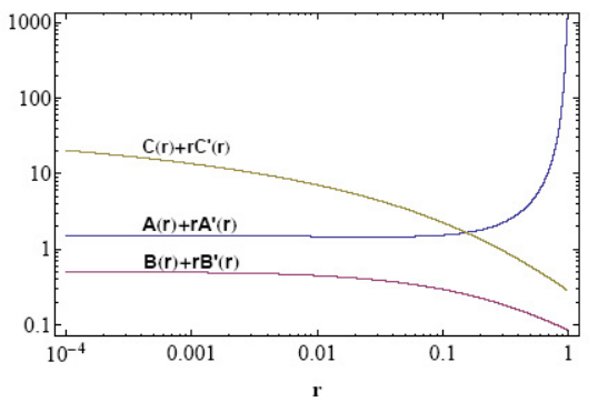
where is the diagonal element of the corresponding trilinear matrix (factoring out the Yukawa coupling) in the super-CKM basis. In the expression, the function for gluinos and for charginos and neutralinos. The function and are loop functions defined in the Appendix II. One can see that decreases rapidly as when the squark masses increase. However, the function behaves differently for different particles () in the loop. Due the gaugino and squark mass hierachy, is small. From Fig. 2, we can see that is enhanced in the small region compared to other functions which remain small. Therefore, the gluino contribution dominates the quark CEDM. For the quark EDM, it is given by a similar expression as (29) but now the quantity is determined only by and . In particular, is determined solely by for and in the loop, and by a combination of and for in the loop. Since and are much smaller than as seen from Figure 2, the quark EDM contributions to the neutron EDM are negligible compared to that of the quark CEDM contributions. Therefore, we only need to calculate the quark CEDM, for which the gluino diagram gives the dominant contribution as explained above. Since in the M-theory framework, one obtains:
| (30) |
Based on the quark EDM and CEDM, the neutron EDM can be computed from (26):
| (31) |
Similarly, the mercury EDM is
| (32) |
Moving on to the electron EDM, it can be computed at leading order from the one-loop neutralino and chargino diagrams. First, we notice that the chargino diagram does not contribute in our framework. This is because the fact that the -term phase11 1 Here we have set by a rotation. and the gaugino phases are zero and there is no phase in the chargino mixing matrix as can be seen from Eq.(49) in the Appendix. The neutralino contribution, on the other hand, gives rise to a non-zero contribution because of a dependence on the selectron mixing parameters (which contains CP-violating phases) in its couplings (see Eq. (50)). Given the fact that the higgsino coupling to electron and selectron is suppressed by the small electron Yukawa coupling, and the wino does not couple to right-handed fermions and sfermions, the dominant contribution is from the diagram with (almost pure bino in the M-theory framework), which can be calculated using Eq. (53) in the Appendix. Thus, the electron EDM is given by:
| (33) |
V.2 Two-loop Contributions
So far, we have considered the one-loop contribution to quark and electron EDMs (and/or CEDMs). In addition, there are two-loop Barr-Zee type contributions [38, 39, 40, 41, 42, 43, 44, 45, 46] such as the one in Fig. 3. In general, the Barr-Zee type diagrams can involve squarks, charginos or neutralinos in the inner loop, and higgs bosons (neutral or charged) and/or gauge bosons in the outer loop (the two-loop diagram considered in split supersymmetry is not relevant here, since there the CP violation is not from trilinear couplings, but instead from the chargino sector). Since only the trilinear couplings contain CP-violating phases in our framework, we consider those diagrams with squarks running in the inner loop as seen in Figure 3. One might wonder whether there are any two-loop diagrams that would contribute if there were phases in the gaugino masses or term such as in the split supersymmetry scenario[45, 58]. Since the higgsino in the M-theory framework is very heavy with mass and hence decoupled from the low energy theory, the only diagram which might contribute is the one in Fig. 4. However, it turns out that the CP phases in the two W-chargino-neutralino couplings cancel out (up to a small correction due to the heavy higgsino) in the final result giving no EDM contribution.


When the mass splitting between the two third generation squarks is not particularly large, the diagram to the quark CEDM can be estimated as (see Appendix C):
| (34) | |||||
where () for (), with third generation squark mass and the pseudoscalar mass of . Here we have used (24) for . For simplicity, we also take . It can be seen that the result of the Barr-Zee diagram to quark CEDM (similar for EDM) is negligibly small. One of the reasons is that CP violation in the third generation is suppressed by about two orders of magnitude as in (24). Similarly, for the electron EDM the result is:
| (35) |
which is again quite suppressed. This contribution may be enhanced for large as seen from above. The M-theory framework, however, generically predicts [14].
The neutron EDM could also get a contribution from the dimension six pure gluonic operator (Weinberg operator), which can be generated from the two loop gluino-top-stop and gluino-bottom-sbottom diagrams. For the case where CP violation only comes from the soft trilinear couplings, the result can be estimated by [59]
| (36) |
where for , and for . The two-loop function is given in [59]. This gives a contribution to the neutron EDM for TeV, GeV and TeV. Thus the neutron EDM from the Weinberg operator is smaller than the one-loop CEDM contribution. However, when the masses of the third generation squarks and trilinears are around TeV, the contribution to the neutron EDM can be significantly larger, and be comparable to the one-loop result.

To summarize our results, we have calculated the EDMs arising from the CP-violating phases in the trilinear terms in a general framework with light gauginos and heavy sfermions, and the results are within current experimental bounds. We find that the one-loop diagram is typically the dominant contribution to EDMs. However, in contrast to the situation in which gaugino and sfermion masses are comparable, the one-loop diagram with gluino is enhanced over the one with neutralino. This leads to a larger ratio between neutron EDM and electron EDM of . In typical supersymmetric models with gaugino and sfermion masses of the same order, this ratio is [60]. This seems to be a robust feature of models in which the gauginos are suppressed relative to the squarks and the trilinears and the trilinears are not proportional to Yukawas. Finally, it is easy to see that the mercury EDM provides the most stringent limit on the squark masses. For squark masses around TeV, the mercury EDM will increase to , which could be tested in the near future with better experimental precision. Basically, we have found that the upper bounds on the EDMs in the M-theory framework result from two of its generic features - large scalar masses and trilinears ( TeV), and CP-violating phases only in the trilinear couplings and those arising only from the Yukawas.
VI Higher-Order Corrections
In Section II, we found that there are no CP-violating phases from supersymmetry breaking at leading order in the framework of M-theory compactifications considered. It is therefore important to check if corrections to the Kähler potential and superpotential lead to further contributions to CP-violating phases in the soft parameters and in turn to the EDMs. Although the detailed form of possible corrections is not known in M-theory, some general arguments can neverthless be made, which strongly suggest that higher order corrections still naturally suppress CP-violating phases.
The corrections to the soft parameters may arise in general from corrections in the superpotential and the Kähler potential. In the zero flux sector which we have considered, the superpotential may only receive additional non-perturbative corrections from strong gauge dynamics or from membrane instantons. As mentioned in section II.2 and explained in Appendix (A), the dynamical alignment of phases still works if these additional terms are subdominant compared to the first two terms. The subdominance of these additonal terms is required anyways to keep the results of the moduli stabilization mechanism intact and hence the consistency of the whole approach. Moreover, it also provides an elegant dynamical solution to the strong CP problem within string theory [24].
Th Kähler potential for the hidden sector comprising the moduli and hidden matter fields on the other hand receives perturbative corrections such as terms with higher powers of as there is no non-renormalization theorem for the Kähler potential. However, the field is composed of elementary quark fields which are charged under the hidden gauge group. Therefore, higher order corrections must be functions of or in order to be gauge invariant. When written in terms of , these corrections are always functions of . This structure is important for our claim of small CP-violating phases since it does not introduce any new phases in the soft parameters. In addition, the perturbative corrections to the Kähler potential are always functions of , which do not lead to any CP violating phases in the soft terms as argued in section II.2. The dependence on is a reflection of the shift (PQ) symmetry of the axion , where . This symmetry is only broken by exponentially suppressed non-perturbative effects [61, 62]. This implies that upto exponentially suppressed contributions, the corrections to the Kähler potential do not give rise to any CP violating phases in the soft terms. Thus, although it is very hard in general to compute the form of corrections in M-theory, the result that the CP violating phases in soft parameters are highly suppressed should be quite robust as it only relies on symmetries.
VII Conclusions
In this paper, we have discussed CP violation in theories arising from fluxless M-theory compactifications with low energy supersymmetry and all moduli stabilized. We have found that the supersymmetry breaking dynamics is CP conserving (up to exponentially suppressed effects). The gaugino masses, scalar masses, and parameters are real at the GUT scale and remain real at the Electroweak scale since RG evolution does not introduce new CP-violtaing phases. However, the full trilinear couplings manage to pick up CP-violating phases from the Yukawa couplings as the trilinear matrices are not proportional to the Yukawa matrices. In addition, RG effects mix the phases between different flavors.
Given a model of Yukawas, therefore, one can estimate the effects of these phases of Yukawas on the trilinear couplings, and therefore on the EDMs. Since hierarchical Yukawa textures are well motivated within this framework, we compute EDMs for such textures. The other relevant feature of the low energy theory is that the scalar masses and trilinears are naturally of due to the absence of sequestering generically. Morover, these scalar masses and trilinears are naturally of TeV) since this is the natural scale of the gravitino mass within the M-theory framework. These two features naturally give rise to small CP-violating effects consistent with experimental limits.
We have estimated the electron, neutron and mercury electric dipole moments utilizing the above features, and found that the estimated upper bounds of the EDMs are all within current experimental limits. The estimated upper bound for the mercury EDM is close to the current experimental limit and could be probed in the near future. A robust prediction of the framework is the existence of a hierarchy of about three orders of magnitude between the neutron and electron EDMs. This essentially results from the mass hierarchy between gauginos and scalars as predicted within M-theory [13], and provides an additional means to test the framework.
It should be emphasized that our results for EDMs are based on the result that the CP-violating phases are entirely from the Yukawas, and therefore, any experimental result which indicates other significant sources of phases would contradict and rule out this approach. We also discuss effects of possible corrections to the Kähler potential and superpotential, and the generalization to other string compactifications.
Note that our results are largely independent of a full solution to the flavor problem. Our results have been derived using the fact that the squark matrices are approximately flavor diagonal at low energies which is naturally predicted within the M-theory framework, as explained in section II.1. Therefore, any solution to the flavor problem consistent with the above feature is consistent with our results.
The quark Yukawas give the CKM phases, and the lepton Yukawas the PMNS phases. The latter can provide the phases needed for baryogenesis via leptogenesis consistent with the above framework, for example as described in [63]. So even with no phases from the soft supersymmetry breaking this framework can give a complete description of all known CP violation.
Acknowledgements.
We would like to thank Bobby Acharya, Nima Arkani-Hamed, Konstantin Bobkov, Jacob Bourjaily, Lisa Everett, Eric Kuflik, Arjun Menon, Brent Nelson, Aaron Pierce and Liantao Wang for useful discussions. PK would also like to thank the Michigan Center for Theoretical Physics (MCTP) for their hospitality where part of the research was conducted. The work of GLK and JS is supported in part by the Department of Energy. The work of PK is supported by DOE under contract no. DE-AC02- 05CH11231 and NSF grant PHY-04-57315.Appendix A Dynamical Alignment of Phases in the Superpotential
The dynamical alignment of phases is crucial for solving the SUSY CP problem in the M-theory framework. It means that terms in the moduli superpotential dynamically align to acquire the same phase in the vacuum (perhaps up to exponentially suppressed effects), implying that the superpotential in the vacuum becomes real after rotating away the unphysical overall phase.
It was shown in [13, 14] that with just two non-perturbative contributions (“double condensate terms”) in the superpotential, all moduli, the meson field, and one axion can be fixed in the supergravity regime with both terms in the superpotential acquiring a common phase in the vacuum. At this level, however, all but one axions remain unfixed. This is because the supergravity scalar potential only depends on one linear-combination of axions, while it depends on all the moduli (through the Kähler derivative). It is important to stabilize the remaining axions in a way such that the superpotential becomes (dominantly) real in the vacuum.
Precisely such a mechanism to stabilize the axions has been recently studied in [24]. There, it was shown that higher order terms in the superpotential, which depend on the remaining linear combinations of axions, can stabilize these axions. The superpotential is then given by:
| (37) |
where we have assumed that the subdominant terms in (37) arise from string instantons or gaugino condensates in pure Super Yang-Mills hidden sectors. It is possible to include matter in the hidden sectors as well, but that will not change the qualitative results obtained. In order to keep the original moduli stabilization mechanism and the resulting analysis of [13, 14] intact, the “double condensate” terms must be parametrically larger than these higher order terms. This can be naturally obtained when . It turns out that this will also make the superpotential real in the vacuum (up to exponentially suppressed effects), as shown below.
It is easy to see that in the supergravity potential, the dominant terms arise from the first two terms in (37). Following [13], the dependence of the dominant potential on the axions is given by:
| (38) | |||||
where , , , and , , , are positive coefficients independent of the axions. Thus, the axion combination is minimized at
| (39) |
while the remaining axion combinations stay unfixed.
Now, including other terms in the superpotential such that the “double condensate” approximation is valid, one finds that the remaining axions are stabilized by the next largest terms in the scalar potential depending on those linearly independent combinations of axions. These terms are generated by the product of one of the two dominant terms and one of the subdominant terms. To compute the stabilized values of the axion combinations it is useful to write the effective potential for light axions after integrating out the moduli, meson field and one axion combination which receive a mass of . This is given by [24]:
| (40) | |||||
where are O(1) coefficients. This implies that the axion combinations are all stabilized such that:
| (41) |
depending on whether is negative or positive respectively. In terms of , the full superpotential can thus be written as:
which is (dominantly) real up to one overall phase. The phases of other possible terms present in the superpotential (denoted by … above) will be completely determined by the stabilized axions above, and may be different from 0 or . However, since these terms are exponentially suppressed relative to the dominant terms, one finds that after rotating away the unphysical overall phase the superpotential is real in the vacuum up to exponentially suppressed effects.
Note that for the above mechanism to work it is crucial that the terms in the superpotential which stabilize all moduli and one combination of axions, are dominant compared to the remaining terms. In the case studied in this paper this amounts to having the first two terms in the superpotential dominant compared to other ones. If many or all terms are comparable to each other, the analysis becomes more complicated and the axion combinations are then generically stabilized at a non-trivial value other than 0 or implying that the superpotential is not real in the vacuum.
Another consequence of the above result which has been studied in [24] in detail, is that these light axion mass eigenstates are exponentially lighter compared to the moduli, meson and heavy axion which are . This allows for a beautiful dynamical solution to the strong CP problem within string theory and explicitly realizes the string axiverse scenario considered in [64]. It is remarkable that the mechanism which stabilizes the axions in the framework considered in [24] and solves the strong CP problem automatically stabilizes them in such a way that the superpotential is (dominantly) real in the vacuum.
The above result also applies to other classes of string compactifications. For example, it was shown in [25] that within certain classes of Type IIB flux compactifications, all kähler moduli and one of their axion partners can be stabilized with a superpotential with a constant term and just one non-perturbative contribution which depends on a linear combination of all moduli, i.e. for
| (42) |
All but one axions remain massless at this level. If these axions are stabilized by subdominant terms in the superpotential, this would give rise to the same conclusion in these compactifications as well.
Appendix B The leading one-loop contributions to EDM
The fermion EDMs can be generated at one-loop in supersymmetric models with CP-violating phases in the soft supersymmetry breaking sector. Within the framework considered in this paper, the CP-violating phases only reside in the trilinear terms and therefore appear in the mass mixing terms of the left- and right-handed sfermions. Therefore, the main contribution to the quark EDM and CEDM comes from diagrams involving gluinos because of the large gauge coupling. For the electron EDM, the dominant contribution comes from the diagram involving neutralinos. This is because the diagrams with charginos in the loop require CP-violating phases in the chargino sector which do not arise within the M-theory framework considered.
Let us first consider the diagrams contributing to quark EDM and CEDM with gluino running in the loop
| (43) | |||||
| (44) |
where and is the matrix which diagonalizes the squark mass matrix
| (45) |
More explicitly
| (46) |
Here and are loop functions defined as:
In the above equations, we assume no flavor mixing in the squark mass matrices as argued in the main body of the paper. Using the fact that , we have:
| (47) |
Similarly
| (48) |
In the calculation above, we assume the mass splitting of squarks is small compared to the squark mass. This is usually true since we are only interested in the up and down squarks. When , one finds that . It is easy to see that . For other diagrams which involve neutralino and charginos, the structure is very similar. However, they are much smaller than and can be neglected.
Now let us turn to the one-loop diagrams contributing to the electron EDM
| (49) | ||||
| (50) |
where , and
Here we have
| (51) |
The loop function is given by
| (52) |
In the above equations, , and are the conventional chargino, neutralino and selectron mixing matrices. It is easy to see that the chargino diagram do not contribute to the electron EDM in the framework considered, since there is no CP-violating phases in the chargino sector. In the absence of the neutralino mixing, the expression of can be significantly simplified
| (53) |
where with denoting the average mass of the selectrons. In the above result, the higgsino contribution is neglected since it is suppressed by the small .
Appendix C Barr-Zee diagram
As we have discussed in subsection V.2, we are concerned with the Barr-Zee diagram with the third generation squarks, i.e. and , running in the inner loop. Here we give the detailed derivation of Eq. (34) and (35). We start with the general results of EDM and CEDM for the Barr-Zee diagram [40]
| (54) |
where is the mass of pseudoscalar higgs , , () for () and is the two-loop function
| (55) |
The CP-violating couplings are given by
| (56) |
where are the stop and sbottom mixing angles, and . The mixing angle of the squark sector is given by
| (57) | |||||
Therefore, Eq. (56) becomes
| (58) |
Using Eq. (56) and (57), we can rewrite Eq. (54) as
| (59) | |||||
where and with being the average masses of the stops and sbottoms respectively.
References
- [1] C. A. Baker et al., Phys. Rev. Lett. 97, 131801 (2006), eprint hep-ex/0602020.
- [2] P. G. Harris et al., Phys. Rev. Lett. 82, 904 (1999).
- [3] B. C. Regan, E. D. Commins, C. J. Schmidt, and D. DeMille, Phys. Rev. Lett. 88, 071805 (2002).
- [4] M. V. Romalis, W. C. Griffith, and E. N. Fortson, Phys. Rev. Lett. 86, 2505 (2001), eprint hep-ex/0012001.
- [5] W. C. Griffith et al., Phys. Rev. Lett. 102, 101601 (2009).
- [6] A. Masiero and L. Silvestrini (1997), eprint hep-ph/9709242.
- [7] S. Abel, S. Khalil, and O. Lebedev, Nucl. Phys. B606, 151 (2001), eprint hep-ph/0103320.
- [8] T. Ibrahim and P. Nath, Phys. Lett. B418, 98 (1998a), eprint hep-ph/9707409.
- [9] T. Ibrahim and P. Nath, Phys. Rev. D57, 478 (1998b), eprint hep-ph/9708456.
- [10] T. Ibrahim and P. Nath, Phys. Rev. D58, 111301 (1998c), eprint hep-ph/9807501.
- [11] M. Brhlik, G. J. Good, and G. L. Kane, Phys. Rev. D59, 115004 (1999), eprint hep-ph/9810457.
- [12] B. S. Acharya, K. Bobkov, G. Kane, P. Kumar, and D. Vaman, Phys. Rev. Lett. 97, 191601 (2006), eprint hep-th/0606262.
- [13] B. S. Acharya, K. Bobkov, G. L. Kane, P. Kumar, and J. Shao, Phys. Rev. D76, 126010 (2007), eprint hep-th/0701034.
- [14] B. S. Acharya and K. Bobkov (2008), eprint 0810.3285.
- [15] K. Choi, Phys. Rev. Lett. 72, 1592 (1994), eprint hep-ph/9311352.
- [16] J. P. Conlon, JHEP 03, 025 (2008), eprint 0710.0873.
- [17] S. Abel, S. Khalil, and O. Lebedev, Phys. Rev. Lett. 89, 121601 (2002), eprint hep-ph/0112260.
- [18] J. L. Bourjaily (2009a), eprint 0905.0142.
- [19] M. Atiyah and E. Witten, Adv. Theor. Math. Phys. 6, 1 (2003), eprint hep-th/0107177.
- [20] J. L. Bourjaily (2009b), eprint 0901.3785.
- [21] I. Affleck, M. Dine, and N. Seiberg, Nucl. Phys. B241, 493 (1984).
- [22] T. Friedmann and E. Witten, Adv. Theor. Math. Phys. 7, 577 (2003), eprint hep-th/0211269.
- [23] B. S. Acharya and S. Gukov, Phys. Rept. 392, 121 (2004), eprint hep-th/0409191.
- [24] B. S. Acharya, K. Bobkov, and P. Kumar (2010), eprint 1004.5138.
- [25] K. Bobkov, V. Braun, P. Kumar, and S. Raby (2010), eprint 1003.1982.
- [26] J. A. Bagger, T. Moroi, and E. Poppitz, JHEP 04, 009 (2000), eprint hep-th/9911029.
- [27] A. Brignole, L. E. Ibanez, and C. Munoz (1997), eprint hep-ph/9707209.
- [28] G. F. Giudice and A. Masiero, Phys. Lett. B206, 480 (1988).
- [29] D. J. H. Chung et al., Phys. Rept. 407, 1 (2005), eprint hep-ph/0312378.
- [30] E. Witten (2001), eprint hep-th/0108165.
- [31] B. S. Acharya and E. Witten (2001), eprint hep-th/0109152.
- [32] P. Berglund and A. Brandhuber, Nucl. Phys. B641, 351 (2002), eprint hep-th/0205184.
- [33] N. Arkani-Hamed and M. Schmaltz, Phys. Rev. D61, 033005 (2000), eprint hep-ph/9903417.
- [34] E. A. Mirabelli and M. Schmaltz, Phys. Rev. D61, 113011 (2000), eprint hep-ph/9912265.
- [35] D. E. Kaplan and T. M. P. Tait, JHEP 11, 051 (2001), eprint hep-ph/0110126.
- [36] H. Abe, K. Choi, K.-S. Jeong, and K.-i. Okumura, JHEP 09, 015 (2004), eprint hep-ph/0407005.
- [37] C. D. Froggatt and H. B. Nielsen, Nucl. Phys. B147, 277 (1979).
- [38] S. M. Barr and A. Zee, Phys. Rev. Lett. 65, 21 (1990).
- [39] D. Bowser-Chao, D. Chang, and W.-Y. Keung, Phys. Rev. Lett. 79, 1988 (1997), eprint hep-ph/9703435.
- [40] D. Chang, W.-Y. Keung, and A. Pilaftsis, Phys. Rev. Lett. 82, 900 (1999), eprint hep-ph/9811202.
- [41] A. Pilaftsis, Phys. Lett. B471, 174 (1999), eprint hep-ph/9909485.
- [42] D. Chang, W.-F. Chang, and W.-Y. Keung, Phys. Lett. B478, 239 (2000), eprint hep-ph/9910465.
- [43] D. Chang, W.-F. Chang, and W.-Y. Keung, Phys. Rev. D66, 116008 (2002), eprint hep-ph/0205084.
- [44] A. Pilaftsis, Nucl. Phys. B644, 263 (2002), eprint hep-ph/0207277.
- [45] D. Chang, W.-F. Chang, and W.-Y. Keung, Phys. Rev. D71, 076006 (2005), eprint hep-ph/0503055.
- [46] Y. Li, S. Profumo, and M. Ramsey-Musolf, Phys. Rev. D78, 075009 (2008), eprint 0806.2693.
- [47] M. Pospelov and A. Ritz, Annals Phys. 318, 119 (2005), eprint hep-ph/0504231.
- [48] A. Manohar and H. Georgi, Nucl. Phys. B234, 189 (1984).
- [49] R. L. Arnowitt, J. L. Lopez, and D. V. Nanopoulos, Phys. Rev. D42, 2423 (1990).
- [50] R. L. Arnowitt, M. J. Duff, and K. S. Stelle, Phys. Rev. D43, 3085 (1991).
- [51] D. A. Demir, O. Lebedev, K. A. Olive, M. Pospelov, and A. Ritz, Nucl. Phys. B680, 339 (2004), eprint hep-ph/0311314.
- [52] T. Falk, K. A. Olive, M. Pospelov, and R. Roiban, Nucl. Phys. B560, 3 (1999), eprint hep-ph/9904393.
- [53] V. Baluni, Phys. Rev. D19, 2227 (1979).
- [54] R. J. Crewther, P. Di Vecchia, G. Veneziano, and E. Witten, Phys. Lett. B88, 123 (1979).
- [55] M. Pospelov and A. Ritz, Phys. Rev. Lett. 83, 2526 (1999), eprint hep-ph/9904483.
- [56] J. P. Archambault, A. Czarnecki, and M. Pospelov, Phys. Rev. D70, 073006 (2004), eprint hep-ph/0406089.
- [57] M. E. Pospelov and I. B. Khriplovich, Sov. J. Nucl. Phys. 53, 638 (1991).
- [58] G. F. Giudice and A. Romanino, Phys. Lett. B634, 307 (2006), eprint hep-ph/0510197.
- [59] J. Dai, H. Dykstra, R. G. Leigh, S. Paban, and D. Dicus, Phys. Lett. B237, 216 (1990).
- [60] S. Abel and O. Lebedev, JHEP 01, 133 (2006), eprint hep-ph/0508135.
- [61] E. Silverstein, Phys. Lett. B396, 91 (1997), eprint hep-th/9611195.
- [62] I. Antoniadis, B. Pioline, and T. R. Taylor, Nucl. Phys. B512, 61 (1998), eprint hep-th/9707222.
- [63] P. Kumar (2008), eprint 0809.2610.
- [64] A. Arvanitaki, S. Dimopoulos, S. Dubovsky, N. Kaloper, and J. March-Russell (2009), eprint 0905.4720.