Hybrid Quintessential Inflation
Abstract
A model is presented in which a single scalar field is responsible for both primordial inflation at early times and then dark energy at late times. This field is coupled to a second scalar field which becomes unstable and starts to oscillate after primordial inflation, thus driving a reheating phase that can create a high post-inflation temperature. This model easily avoids overproduction of gravity waves, which is a problem in the original quintessential inflation model in which reheating occurs via gravitational particle production.
pacs
98.80.Cq, 95.36.+xI Introduction
Peebles and Vilenkin proposed in [1] that both inflation and dark energy could be a result of the same scalar field, with vacuum expectation value , interacting only with gravity and itself via the potential term , which they chose to be
| (1) |
At tree level the evolution of the vacuum expectation value of the -field is governed by
| (2) |
with the cosmological expansion rate related to energy density by the Friedmann equation,
| (3) |
where the Planck mass GeV and overdots signify derivatives with respect to coordinate time.
In the original scenario [1], the universe begins dominated by the potential energy of the scalar field . The field has some large, negative value, and slowly rolls toward the origin. The slow-roll conditions of inflation are satisfied, and the universe expands exponentially. During inflation, fluctuations in are frozen into the field. These seed future structure in the universe. To provide the correct level of fluctuations, as usual . When , the inflationary epoch draws to a close. Thus far the situation is identical to chaotic inflation [2], but from here on it differs. The kinetic energy of the field is no longer negligible, and it soon begins to dominate the universe [3]. This phase is termed “kination”. The field behaves approximately as stiff matter, with its energy density redshifting as . Taking the potential energy at the end of inflation to be the same as the kinetic energy, a simple estimate gives
| (4) |
with solution, and thus . Here the subscript indicates the value at the end of inflation. During this kinetic dominated phase, the field moves as
| (5) |
Thus, spacetime started in approximately de Sitter form, and ended dominated by the kinetic energy of a homogeneous field. Ford showed [4] this transition leads to gravitational particle production. The result is a small but important energy density of relativistic particles,
| (6) |
where is the number of scalar fields. Thermalization was found in [1] to occur at a radiation temperature
| (7) |
The radiation redshifts away slower than the energy in the field. Provided in Eq. (1) is not too large, Peebles and Vilenkin showed the universe transitions to a radiation dominated epoch, with a temperature of
| (8) |
The field remains essentially static from this point on, mimicking a cosmological constant. The value of can be then chosen so that matches today’s observed value of dark energy density. In the analysis in [1], this turned out to be GeV.
Unlike most inflationary scenarios, in the one by Peebles and Vilenkin [1] at the end of inflation the inflaton field does not undergo a series of damped oscillations about a potential minima, which is the mechanism by which reheating usually takes place [5]. The absence of this behaviour means gravitational particle production has to be relied upon instead. The same gravitational mechanism works to produce a stochastic background of gravitational waves (GW) [6, 7, 8], and the overproduction of gravity waves is one of the potential dangers of this model. Gravitons behave as minimally massless scalar fields, and the energy density of the gravitons by the end of inflation is just that of a single scalar field, times two polarization states, so that the ratio of the energy densities in GW to radiation at the end of inflation is simply . At the time of nucleosynthesis will contribute as an effective extra degree of freedom in radiation, but the success of Big Bang Nucleosynthesis (BBN) in predicting the abundances of light elements puts a constraint on the extra number of light degrees of freedom, be those neutrinos species or gravitons, such that ; tracing back the evolution of this ratio upto the start of the kination period this would sets a lower bound [1].
The problem of gravity waves overproduction is quite generic in models of inflation followed by a long period of kination [9], or in general stiff matter domination [10], like brane world inflation [11]. To allow for a more effective reheating process, able to suppress the relative contribution of the GW at the time of BBN, one can invoke alternative methods like instant preheating [12], curvaton reheating [13], or Born-Infeld reheating [14]. Any alternative implies introducing extra scalar degrees of freedom at the time of inflation, like in curvaton reheating, and/or direct couplings of the inflaton field to the light degrees of freedom as in instant preheating.
In this letter we explore the possibility of a simpler scenario, recovering a more typical reheating mechanism driven by the decay of an oscillating massive field [5]. We extend Peebles and Vilenkin model by a new scalar field coupled to the inflaton field [15] with a hybrid-like potential [16]. In our scenario, once the inflaton field falls below a critical value, the field can start oscillating, thus gaining energy that afterwards can be converted into radiation through perturbative decay, as in the usual reheating mechanism. However, in contrast to the standard reheating picture, in our scenario reheating takes place during kination instead of the more standard matter domination. Unless the perturbative decay of the field is tiny, this results in a larger reheating than in the original model of Peebles and Vilenkin [1], and a shorter kination phase. The more efficient reheating also ensures that radiation domination takes over kination, well before the inflaton vacuum energy starts dominating again.
This letter is organized as follows. In Section II the potential and parameters of the model are set. Also the general behaviour is described of the field after inflation, when it can oscillate and drive reheating. The reheating temperature is then computed in Section III. For the mechanism to work, we need to check first that indeed oscillates when the inflaton field passes through the critical point, and that it does not backreact on the evolution of . Fulfilling these conditions sets the constraints on the model parameters, which are given in Section IV. In Section V we present the range of consistent with the constraints. The transition to a radiation dominated universe is studied in Section VI. Once the constraints are fulfilled, the transition before the onset of dark energy domination is practically ensured. As this is a hybrid-like model, we comment on the issue of domain walls in section VII. Finally in Section VIII we present the summary and future work related to quantum corrections.
II General behaviour of the hybrid field
To enable once more the standard reheating, we introduce a new scalar field , that we couple to the inflaton field. The effective potential at tree-level is
| (9) |
where is the potential given by equation (1). The parameters , , and are as yet undetermined constants. Note that when is relaxed near the origin, .
The -field is assumed to be located somewhere near its minima at . As the field evolves from large negative values to large positive ones, the turning point at the origin temporarily becomes unstable for the -field, and two minima are generated on either side. The position of the minima, are given by
| (10) |
They exist only while . The bottom of the well is at a negative value of potential energy. This is a result of how the energy of the system has been defined. It has no physical consequence for the present scenario, since the total energy density will always remain positive, as it is dominated by the kinetic inflaton energy density.
The -field has a characteristic response time to react to changes in the potential. This can be estimated as , provided is not too close to . If changes in the potential take place quicker than this response time, the field will have no chance to react. For instance, if moves between and in a time throughout, will have no time to move before the origin becomes a stable minima once more. On the other hand, if the changes take place on timescales that are much longer than the response time, i.e. , the field will be able to relax into the minima very quickly. If this is the case throughout, there will hardly be any oscillations (and hardly any reheating).
A fact alleviates the above difficulties: is slowing down, and is doing so quickly (its evolution is logarithmic in time). This means the timescale becomes gradually longer. Furthermore, the timescale that governs how quickly reacts is not static. It is longest when and is shortest at . We will take the view that the field begins to move before . This places an immediate constraint on the model parameters: . We should immediately note the better this inequality is satisfied, the sooner will start to move after becoming unstable. This will limit the amount of energy for its oscillations.
As a simplified picture, consider the field to be frozen at the origin up until a time after becoming unstable. Afterwards, the potential will be approximately constant during the fast oscillations of the field. The energy in the oscillations (available for reheating) will then be the depth of the potential well at the point when the field begins to move. This will be some fraction of the maximum potential well depth. The energy available for reheating can then be written:
| (11) |
Eventually, after many oscillations, reaches , and the - field then oscillates about its stable minima at the origin. These oscillations will reheat the universe.
The fraction now needs to be estimated. For this, we assume the -field moves some short time after it becomes unstable, with the instability occurring at . As this time signals the start of reheating, it will be called . Writing the time since the start of reheating as , then we can estimate that the field will begin to move when . In other words, the field moves after it has been unstable for a time approximately the same as its characteristic reaction time (which is itself a function of ). The depth of the well is given by
| (12) |
Comparison with equation (11) shows
| (13) |
with evaluated when . We assume moves only slightly, an amount , before begins to move. Re-writing equation (5) gives
| (14) |
We wish to find the value of satisfying . As , we can insert to find
| (15) |
The same substitution into yields
| (16) |
to leading order in .
Applying the condition , we can find the value of when the - field begins to move. Relating to with equation (14), we finally obtain
| (17) |
Note that this order of magnitude approximation breaks down if begins moving when is not small compared to , signalled by approaching (or exceeding) unity. This expression should not be trusted in such circumstances. Assuming to be small is a slightly stronger constraint than the constraint discussed earlier, that . The former gives the condition the field moves quickly after becoming unstable, the latter is just the condition the field moves at all, at or before . We will return to this point when discussing the parameter constraints in Section IV.
III Reheating temperature
Once , the field will return to the origin. If it acquired kinetic energy due to its temporary displacement, it will now oscillate about the origin. The previous section established the amount of energy expected from these oscillations.
If the oscillations are small, the field can be approximated as undergoing simple harmonic motion. In such a case, the elementary theory of reheating can be applied [5]. In this phenomenological approach, an extra term is added to the equation of motion of the field to account for particle decay. The value of is taken to be the decay rate of the particle. The field then obeys the equation of motion
| (18) |
This approach is valid when the oscillations are small and the oscillations are well approximated as simple harmonic motion. For a more complete picture, valid at the early stages we should also consider the effect of preheating [17] (see also [12] for an analysis of preheating in the context of quintessential inflation). However, these details will be ignored in this paper and we will examine only the simplest reheating estimates.
We stress that this phenomenological approach is only valid while the field is undergoing coherent oscillations about its minima. It will not be valid otherwise, nor over short timescales, and is likely to fail when . For this reason we will consider reheating to take place only while , so that we may have confidence our calculations are always carried out in an appropriate regime.
We assume , and can be taken to be approximately constant over a single oscillation. Equation (18) is re-written by replacing by its value over a complete oscillation, , which is valid for simple harmonic motion. This yields
| (19) |
Assuming the field is still undergoing simple harmonic motion, . Then we can write
| (20) |
This can be solved,
| (21) |
with
| (22) |
We have used subscript to indicate the value of a variable when . From energy conservation, it follows that the radiation density must obey
| (23) |
Imposing the condition there is no radiation at the start of decay, an approximate solution is found by neglecting the exponential decay of . This will be valid up to . After this, the energy in the field will decay rapidly away and the radiation will simply redshift with its usual behaviour.
Inserting our earlier expression for into equation (23), the solution for the radiation energy density can be written as
| (24) | |||||
with and the constant of integration chosen so that there is no radiation at .
Assuming before reaches , the energy density in radiation should be well approximated by
| (25) |
The energy density of the radiation continues growing logarithmically, despite the energy loss from redshifting. This is due to the mild amount of energy being added to the field by its coupling to . It will continue to grow in this way until . If this is a sufficiently late time that the last term in Eq. (25) dominates, then
| (26) |
Once the universe has had chance to thermalize, the temperature is related to the energy density via,
| (27) |
where is the number of degrees of freedom.

Thermalization occurs when the interaction rate becomes comparable to the expansion rate , where is the number density of the light degrees of freedom and the their interaction cross section. We can estimate that the light degrees of freedom are created with a typical energy , and , with being the strength of the mediating interactions. Using Eq. (26) with the expression of given in the next section Eq. (31), and as a typical value for the coupling in the cross-section , one gets that at the beginning of the reheating period,
| (28) |
We have also written the decay rate for a massive particle as , where is the coupling constant mediating the decay, and the mass. For the analyses of the reheating done in this section, the decay rate and therefore the coupling must be such that . For values of the parameters consistent with the constraints given in the following section, this is general the case with . Significantly, with this choice for then Eq. (28) is already larger than one. Therefore, light degrees of freedom thermalized promptly after they are produced.
We have confirmed these approximations are successful in their appropriate regimes by numerically solving this system of differential equations (Friedmann’s equation, the equations of motion for both fields, and the radiation energy density). Figure 1 shows the numerically determined evolution of the - field as it becomes unstable, and the subsequent damped oscillations that reheat the universe.
IV Parameter constraints
We have made two assumptions that can be formulated as simple constraints on combinations of parameters. The first of these is that begins to move toward its new equilibrium at or before . Earlier we noted this condition was . The second assumption is that the field does not significantly influence the motion of the field. It could do this either from the coupling, or from the energy density of the field modifying the expansion rate of the universe.
First we shall calculate . As at , we can use equation (22) with these values inserted. Re-arranging,
| (29) |
and by writing , gives
| (30) |
with the rightmost expression in the case . Thus, it is noteworthy that is a good approximation.
An estimate of is still needed. We use equation (4) and , to write it in terms of a ratio of scale-factors,
| (31) |
where is the scale factor at . The time for to move between and is then given by
| (32) |
The ratio of scale-factors can be found from equation (5). Re-arranging and setting at ,
| (33) |
As such the time interval available can be written simply as
| (34) |
with . Recalling , a constraint on the model parameters can be constructed:
| (35) |
Now that we have an expression for , a constraint on can also be calculated. Replacing Eq. (31) into (17) gives
| (36) |
This is comparable although slightly more restrictive than Eq. (35). This suggests that there can be a region in parameter space where the second constraint is violated (suggesting ) but the first satisfied (so that the field still begins to move out of its unstable position). The resulting reheating temperature in this region is also fairly insensitive to changes in and , compared with when the second constraint is well satisfied (and the reheat temperature influenced by as given by equation (17)). Nevertheless, to ensure that we are in the region of parameter space for which the field has oscillated enough to reheat the universe, when referring to these constraints we will use . Having as the largest possible mass scale in the model , the strength of the - interaction is therefore bounded from below with .
A second constraint exists from the requirement that the field does not influence the motion of the field. First we will consider the requirement the negative potential energy from the coupling term is not significant compared to the kinetic energy of . As the kinetic energy is constantly diminishing, it will be simpler to overestimate the potential energy and underestimate the kinetic energy. We will therefore take the potential energy to be its maximum value, and the kinetic energy to be the value at . No matter the evolution of these quantities, if the quantities evaluated at these two time intervals are not comparable, they never will be. Reading off the kinetic energy from equation (4) and requiring this always greatly exceeds the maximum of the negative potential energy gives,
| (37) |
or
| (38) |
If we choose values to satisfy ,
| (39) |
Now consider the effect of the coupling on the motion of directly. The equation of motion gives
| (40) |
where the kinetic energy is treated as the dominant contribution to energy of the field. The third term is the contribution due to the coupling, and we wish to ensure this is negligible compared to the second. Using equation (3) to express Hubble’s parameter in terms of the kinetic energy , this condition can be written as,
| (41) |
 |
 |
Treating the right-hand side as the average value over oscillations of the field, we can rewrite it using . Writing these energy densities out explicitly, including their evolution with scale-factor gives
| (42) |
The right-hand side will quickly become tiny when . We need only consider the value of when this occurs, and then . Using and Eq. (17) gives:
| (43) |
and thus unless the decay rate is tiny and the reheating period too long, once we fulfill the other constraints this is practically always fulfilled. In other words, having the parameter values such that the field performs some oscillations around the minimum while the expansion rate is dominated by the inflaton kinetic energy, those oscillations will not backreact onto the motion of the inflaton field.
V Range of Temperatures
The constraints show there can be significant variation in the resulting temperature. The energy density depends most sensitively on , and the range this parameter can take is severely constrained by the other parameters. If is too small, must be made small enough to avoid interfering with the evolution of . If is made too small, must be made large enough to ensure the field reacts while it is unstable. For instance, if then can range from at its largest (with ) to (with ), assuming is kept below the Planck scale. Decreasing can constrain it further.
Reheating ends by the time . Plugging Eqs. (31), (17), with and , we have:
| (44) |
Therefore, working for example with and , we find the range
| (45) |
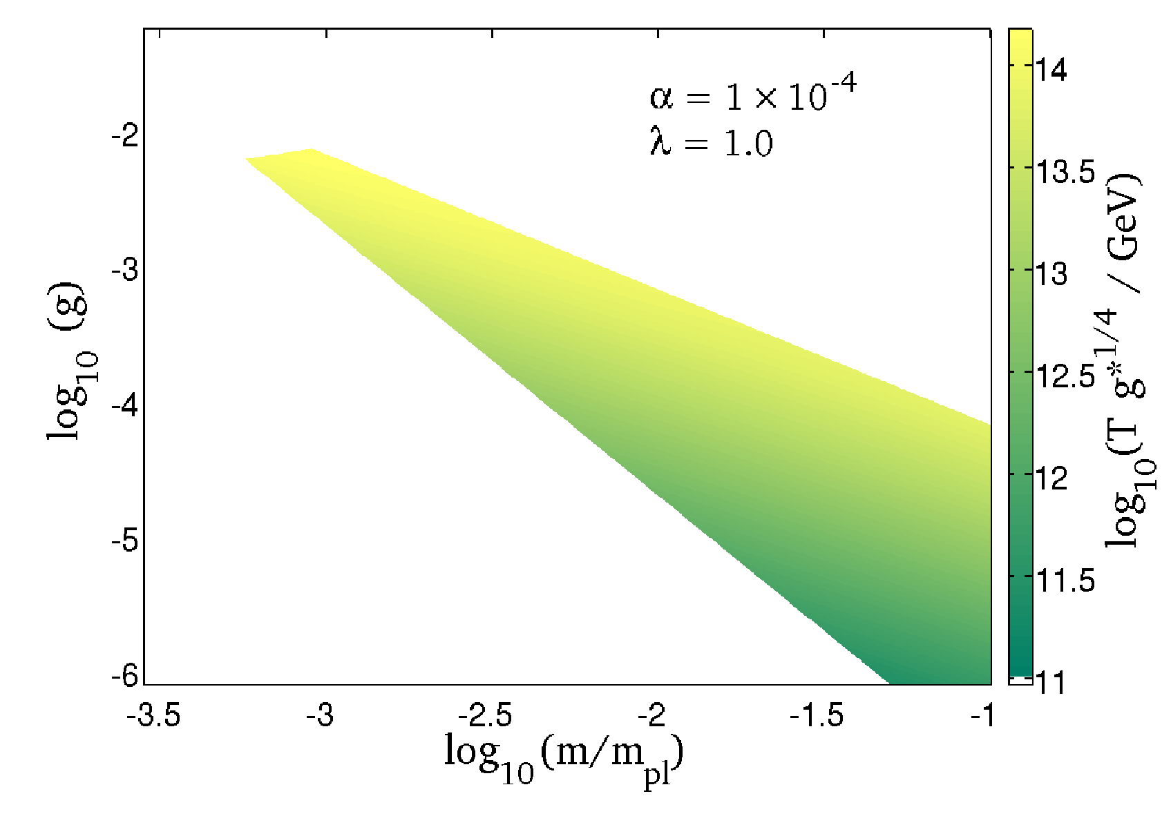
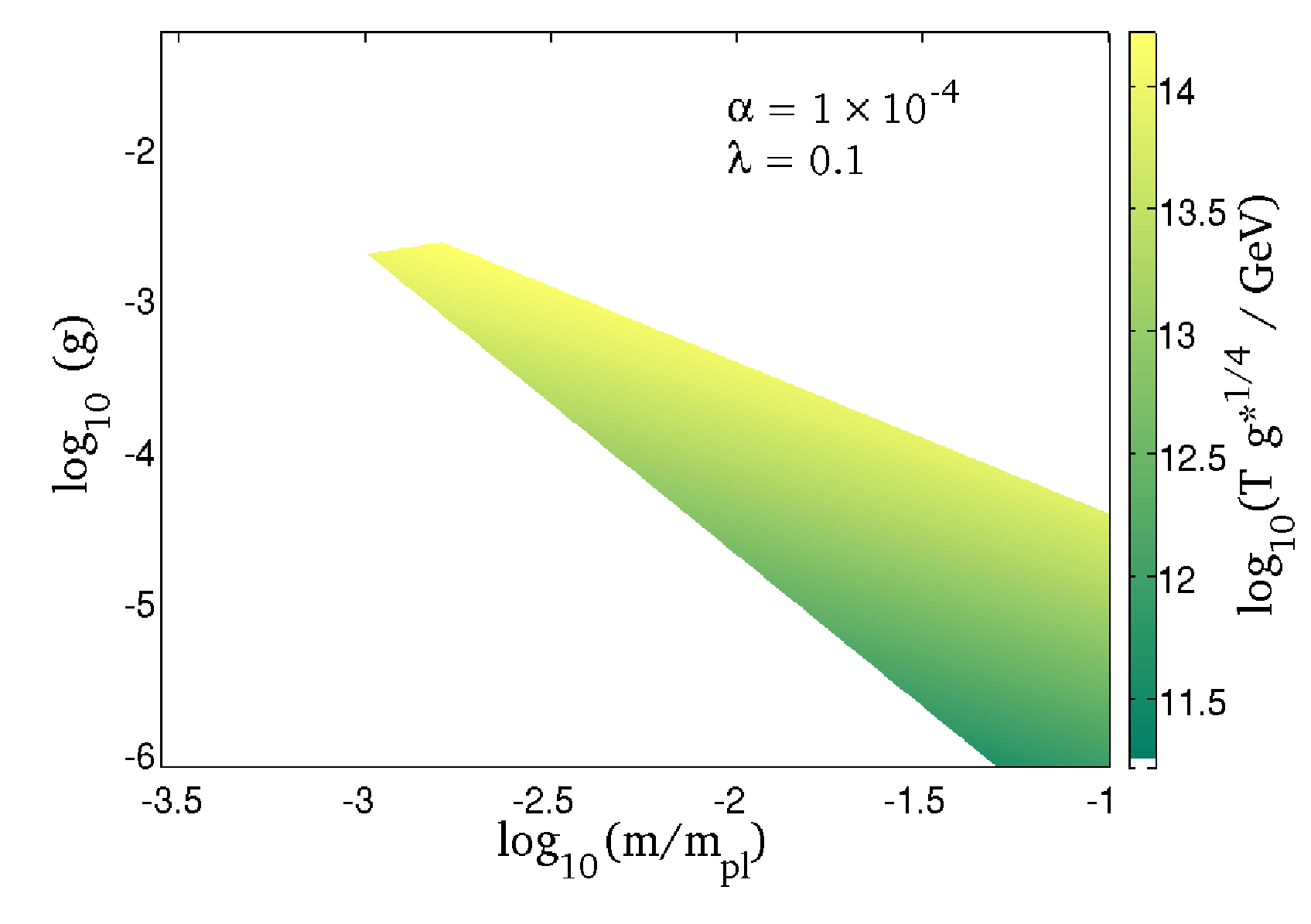
One can also look at very weak coupling, where for example , , , and gives . In Fig. 2 we give the range for the reheating temperature in the plane for two values of . As we decrease the value of the self-coupling, the allowed region in the plane will be further reduced, and that would be the main effect on .
VI Transition to radiation domination
The kinetic energy of the field is dropping quickly. Peebles and Vilenkin noted that unless radiation domination occurred before the kinetic energy reached the potential energy in , the universe would return to an inflationary regime from which it would never recover. Our model has the same requirement. We will write as the scale-factor when reheating ends () and the radiation redshifts as an unsourced relativistic fluid.
The kinetic energy approaches the potential energy at a scalefactor , given by [1]
| (46) |
The energy in the field is
| (47) |
and the energy in the radiation is given in Eq. (44). The ratio is of order unity when the kinetic energy reaches the energy in the radiation, at a scale-factor of . We require to ensure radiation dominated expansion begins. Then,
| (48) |
which is easily satisfied for the values of the parameters we have been considering, but does place a weak upper bound on for a given choice of .
Importantly, the energy in the potential of varies only very slowly. The exact scale-factor , where radiation transition occurs, matters very little in terms of its future evolution: the variation of the field’s potential energy in the range in which this can happen is negligible, as the field is moving so slowly. The same evolution outlined in [1] therefore takes place, with mimicking a cosmological constant and today’s dark energy density obtained with .
VII Domain Walls
Typically in models with a symmetry breaking term, domain walls inevitably form via the Kibble mechanism [18]. Parts of the universe causally separated have no way of being correlated. When the field becomes unstable, in some regions the field will move to positive values, and in other regions to negative values. The domain walls created by the smooth transition between these values are generally a serious problem in many cosmological models, as they can come to dominant the energy density of the universe [19].
Fortunately, and unlike in many models with such an occurrence, the symmetry is restored once . Any walls formed will then dissolve. However, this could leave some effect upon the amount of reheating taking place within the regions of the domain wall, potentially influencing large scale structure formation. As the wall thickness is significantly smaller than a horizon, we do not expect this to be a large effect, but warrants further investigation.
VIII Summary and future discussion
By introducing an additional coupling to a second, self-interacting scalar field, we can restore the traditional reheating mechanisms to the scenario proposed by Peebles and Vilenkin [1]. The symmetry breaking term leaves the field temporarily unstable, which allows it to gain significant amounts of energy. Using a phenomenological approach to reheating, we have calculated the evolution of the relativistic particles produced by the decay of this field. We then described a variety of constraints on the model parameters, ensuring that the additional field does not interfere with the behaviour of the original inflaton. The range in temperature produced is quite narrow if the new field does not strongly self-interact, and the symmetry breaking scale does not reach the Planck scale. But with a self coupling of the order of , one has GeV. This allows us to suppress the contribution of the gravitational waves at the time of BBN well below the upper limit.
With a model that tries to explain the evolution of the Universe from early inflation to today dark energy domination, one of the issues to explain is the origin of the baryon asymmetry [20]. A possibility would be spontaneous baryogenesis through a derivative coupling of the inflaton field to a matter current [21]. In our set-up, due to the larger coupling of to the light degrees of freedom (compared with the gravitational couplings), thermalization occurs promptly after the start of reheating. This opens up the possibility for example of having leptogenesis during or after reheating, by the decay of the lightest right handed neutrino. The field being quite heavy during reheating could decay into the lightest right handed neutrino, or alternatively the neutrinos could be thermally produced.
The model could potentially form domain walls, often causing problems in similar models. In this variation, we note they are transient and do not interfere with future evolution of the universe. The possibility exists their effect upon the reheating temperature will appear as an imprint on large scale structure formation.
The analyses of the reheating mechanism proposed in this letter has been done at tree-level. But having coupled the quintessence field to another scalar field, with a strength , the question arises about the stability of the quintessential potential to quantum corrections. Here we argue that indeed these corrections are under control due to the decoupling theorem, and that the scenario is not spoiled by quantum corrections, but leave the explicit calculation for a future work.
Quantum corrections with the field running in the loops can give rise to a potentially large correction to the quintessence potential, with the one-loop correction given by [22]:
| (49) |
where is the renormalization scale and the field dependent masses, with . So for the field we have a very heavy state that is excited in a universe with an energy density . Given that we do not have enough energy to excite such a heavy states, physically we can expect that they decouple from the spectrum [23], and their contribution to the effective potential is highly suppressed. However, the 1-loop effective potential as given in Eq. (49) is computed using a mass independent renormalization scheme that does not take into account threshold effects. The decoupling would appear naturally when using instead a mass dependent renormalization scheme [24]. To deal with this problem when working with the effective potential one can use instead the “improved” effective potential [25] by replacing all parameters (masses, couplings and field vevs) by their renormalized values in both the tree level and one loop potential, and imposing the physical condition that the potential does not depend on the renormalization scale, . By choosing the renormalization scale below any heavy mass threshold in the model, heavy states decouple and the dependence on is minimised. We are then left with the tree-level potential again with all the parameters evaluated at ,
| (50) | |||||
All possible quantum corrections due to the heavy states are then encoded in the running of the mass parameters and couplings through the renormalization group equations, and are therefore expected to be under control. In future work, we plan to do a detailed analysis of quantum corrections and decoupling in this model.
Acknowledgements.
The work of M.B.G. is partially supported by the M.E.C. under contract FIS2007-63364 and by the Junta de Andalucía group FQM 101. A.B. and B.M.J. acknowledge support from the STFC.References
- [1] P. J. E. Peebles and A. Vilenkin, Phys. Rev. D 59, 063505 (1999).
- [2] A. D. Linde, Phys. Lett. B 129 (1983) 177.
- [3] B. Spokoiny, Phys. Lett. B 315 (1993) 40.
- [4] L. H. Ford, Phys. Rev. D 35 (1987) 2955.
- [5] A. J. Albrecht, P. J. Steinhardt, M. S. Turner and F. Wilczek, Phys. Rev. Lett. 48, 1437 (1982); A. D. Dolgov and A. D. Linde, Phys. Lett. B116 (1982) 329; L. F. Abbott, E. Farhi and M. B. Wise, Phys. Lett. B 117 (1982) 29.
- [6] A. A. Starobinsky, JETP Lett. 30 (1979) 682 [Pisma Zh. Eksp. Teor. Fiz. 30 (1979) 719].
- [7] B. Allen, Phys. Rev. D 37 (1988) 2078.
- [8] V. Sahni, Phys. Rev. D 42 (1990) 453.
- [9] V. Sahni, M. Sami and T. Souradeep, Phys. Rev. D 65 (2002) 023518.
- [10] M. Giovannini, Phys. Rev. D 58 (1998) 083504.
- [11] R. Maartens, D. Wands, B. A. Bassett and I. Heard, Phys. Rev. D 62 (2000) 041301. E. J. Copeland, A. R. Liddle and J. E. Lidsey, Phys. Rev. D 64 (2001) 023509. G. Huey and J. E. Lidsey, Phys. Lett. B 514 (2001) 217.
- [12] A. H. Campos, H. C. Reis and R. Rosenfeld, Phys. Lett. B 575, 151 (2003). M. Sami and V. Sahni, Phys. Rev. D 70 (2004) 083513.
- [13] B. Feng and M. z. Li, Phys. Lett. B 564 (2003) 169. K. Dimopoulos, Phys. Rev. D 68 (2003) 123506. A. R. Liddle and L. A. Urena-Lopez, Phys. Rev. D 68 (2003) 043517.
- [14] M. Sami, N. Dadhich and T. Shiromizu, Phys. Lett. B 568 (2003) 118.
- [15] A. Berera, Pramana 72 (2009) 169.
- [16] A. D. Linde, Phys. Rev. D 49, 748 (1994).
- [17] L. Kofman, A. D. Linde and A. A. Starobinsky, Phys. Rev. Lett. 73, 3195 (1994). L. Kofman, A. D. Linde and A. A. Starobinsky, Phys. Rev. D 56, 3258 (1997).
- [18] T. W. B. Kibble, J. Phys. A 9, 1387 (1976).
- [19] A. Vilenkin and E. P. Shellard, “Cosmic Strings and Other Topological Defects”, Cambridge University Press (1994).
- [20] M. Joyce, Phys. Rev. D 55 (1997) 1875.
- [21] A. De Felice, S. Nasri and M. Trodden, Phys. Rev. D 67, 043509 (2003).
- [22] S. Coleman and E. Weinberg, Phys. Rev. D 7, 1888 (1973); S. Weinberg, Phys. Rev. D 7, 2887 (1973).
- [23] K. Symmanzik, Comm. Math. Phys. 34 7 (1973); T. Appelquist and J. Carazzone, Phys. Rev. D 11, 2856 (1975).
- [24] H. Georgi and H. D. Politzer, Phys. Rev. D 14 (1976) 1829.
- [25] M. Bando, T. Kugo, N. Maekawa and H. Nakano, Phys. Lett. B 301 (1993) 83; M. Bando, T. Kugo, N. Maekawa and H. Nakano, Prog. Theor. Phys. 90 (1993) 405; Nucl. Phys. B 553 (1999) 511.