Dynamic Monte Carlo radiation transfer in SPH.
Radiation
pressure force implementation.
Abstract
We present a new framework for radiation hydrodynamics simulations. Gas dynamics is modelled by the Smoothed Particle Hydrodynamics (SPH), whereas radiation transfer is simulated via a time-dependent Monte-Carlo approach that traces photon packets. As a first step in the development of the method, in this paper we consider the momentum transfer between radiation field and gas, which is important for systems where radiation pressure is high. There is no fundamental limitations on the number of radiation sources, geometry or the optical depth of the problems that can be studied with the method. However, as expected for any Monte-Carlo transfer scheme, stochastic noise presents a serious limitation. We present a number of tests that show that the errors of the method can be estimated accurately by considering Poisson noise fluctuations in the number of photon packets that SPH particles interact with per dynamical time. It is found that for a reasonable accuracy the momentum carried by photon packets must be much smaller than a typical momentum of SPH particles. We discuss numerical limitations of the code, and future steps that can be taken to improve performance and applicability of the method.
Keywords:
Physical Data and Processes: radiative transfer – Physical Data and Processes: hydrodynamics1 Introduction
Astronomers do not have a luxury of testing their ideas of, e.g., galaxy and star formation in a purpose designed laboratory. Instead, testing grounds are provided by observations and numerical simulations. The latter in effect represent experiments with a given set of physical laws included. Clearly, the more physics is included in the simulations the more realistic the latter should be. Presently, two basic physical processes – gravity and hydrodynamics – are modelled well by a variety of methods and codes. For example, one reliable and widely used numerical method of modelling gas dynamics is Smoothed Particle Hydrodynamics (SPH) (Gingold & Monaghan, 1977; Lucy, 1977). It has been used in the various fields of astrophysics, and is especially powerful when resolving high density regions is key. The method is grid-less and fully Lagrangian in nature, facilitating modelling of arbitrary geometry systems. For reviews of the SPH method see, for example, Benz (1990); Monaghan (1992); Fulk (1994); Price (2004).
Radiation transfer and interaction with matter is another basic process operating in astrophysical systems. Starting from the pioneering ideas of Lucy (1977), great efforts have been expended to model radiation–matter interactions in SPH. When gaseous systems modelled are optically thick, photons scatter or get absorbed and re-emitted multiple times before escaping the system (Rybicki & Lightman, 1986). This situation is well approximated by the diffusion approximation. Several authors have already incorporated this radiation transfer scheme in SPH (Lucy, 1977; Brookshaw, 1985; Whitehouse & Bate, 2004; Whitehouse et al., 2005; Whitehouse & Bate, 2006; Viau et al., 2006). The diffusion approximation is usually complemented by a flux limiter method to model optically thin regions where photons stream freely rather than diffuse (Whitehouse & Bate, 2004, e.g.,). Most recently Petkova & Springel (2008) implemented the diffusion radiation scheme in the cosmological code Gadget (Springel, 2005) supplementing it by the variable Eddington tensor as a closure relation.
Ray tracing methods is a principally different approach to radiative transfer, where the radiative transfer equation is solved along chosen directions (rays). Most applications only consider rays that start at discrete sources of radiation field, such as bright stars, etc., essentially neglecting the diffuse radiation field. As far as the density estimation is concerned, some authors used density defined at the locations of the nearest neighbours along the rays (Kessel-Deynet & Burkert, 2000; Dale et al., 2007; Gritschneder et al., 2008), whereas others approximated the density field using the nodes of the tree structure one way or another (Oxley & Woolfson, 2003; Stamatellos & Whitworth, 2005; Susa, 2006). The most recent developments use the SPH density field directly, e.g., c.f. codes SPHRAY (Altay et al., 2008) and TRAPHIC (Pawlik & Schaye, 2008). Ritzerveld & Icke (2006) developed a method to transport radiation on adaptive random lattices, and showed that the algorith is very efficient for cosmological re-ionisation problems.
Monte-Carlo methods are similar in spirit and yet substantially different from the ray tracing codes. In the former, the idea is to discretise the radiation field into “packets”, choose directions and emission time of these packets stochastically to obey proper physical constraints, and then propagate the packets through matter in accord with radiation transfer equations. The main problem for the method is stochastic noise caused by photon packet statistics (Lucy, 1999, for an early SPH application see). Baes (2008) presents some new interesting ideas about using a smoothing kernel in a Monte-Carlo simulation.
Most of these applications were tailored to photo-ionisation problems in the field of star formation or cosmology, where the density field can be considered static as rays propagate through it (Krumholz et al., 2007, the “static diffusion limit”; see ), and where radiation pressure effects can be omitted. There are also a number of radiation transfer codes working with a grid-based hydrodynamics codes rather SPH (Iliev et al., 2006, e.g.,). We do not discuss these methods here.
Here we present and test a new photon packet based radiation transfer scheme combined with an SPH code. The method uses the SPH density field directly, thus preserving the “native” SPH resolution. The previous efforts did not consider the radiation pressure effects, studying instead radiative heating/cooling and photo-ionisation. Here we study the radiation pressure effects instead. We assume that gas equation of state is known (e.g., isothermal or polytrophic) and consider only the radiation pressure forces. This allows us to thoroughly test precision of our approach and numerical noise effects. There is no fundamental difficulty in including the heating/cooling and photoionisation processes in our scheme, and we shall extend our method in that direction in the near future. Another defining characteristic of our new method is that the photon field is evolved in the same time-dependent way, although on shorter time steps, as gas dynamics, and therefore the method is intrinsically time-dependent.
2 Description of the method
2.1 Radiation Transfer Method
Radiative transfer equation along a ray (Rybicki & Lightman, 1986) is
| (1) |
where is the specific radiation intensity, is the opacity coefficient, is gas density and is emissivity of the gas. In general and are functions of direction, radiation frequency, position and time. The first term on the right hand side represents removal of radiation from the beam by absorption and scattering, whereas the last term describes local emission of radiation into the beam’s direction.
In Monte Carlo methods, the radiation field is sampled via photon packets. In the simplest reincarnation of the method, both terms on the right hand side of equation 1 are treated stochastically. The photon mean free path, , is calculated as . A random number, , uniformly distributed over , is generated. A photon is allowed to travel distance , at which point it interacts with gas by passing its energy and momentum to gas completely. The photon is then re-emitted according to physics of a chosen set of radiation processes, and followed again until it escapes the system.
Our radiation transfer scheme is slightly modified from this. Firstly, instead of using discontinuous photon jumps, we explicitly track packet’s trajectory in space as
| (2) |
where and are the current and initial photon locations, and const is the photon propagation speed (not necessarily the speed of light; see §2.5). Secondly, photon momentum, , and photon energy are reduced continuously due to absorption or scattering as
| (3) |
Thus, the first term on the right hand side of equation 1 is treated continuously rather than stochastically. This reduces the statistical noise significantly. Photons are discarded when their momentum drops below a small () fraction of their “birth momentum” .
However, the re-emission term, i.e., the last one in equation 1 is modelled similarly to classical Monte-Carlo methods in that it is stochastic in nature. This is unavoidable in Monte Carlo methods due to the need to employ a finite number of photon packets (Lucy, 1999, e.g.,). In practice, at every photon’s time step , the photon momentum absorbed, , is calculated according to equation 3. As stated in the Introduction, we concentrate in this paper on the radiation pressure effects, and assume that radiation absorbed from the beam is completely re-emitted on the spot in a new random direction. This is the case for pure scattering of radiation or for local radiative equilibrium between radiation and gas. In these cases the amount of momentum (energy) to be re-emitted in the interaction considered is exactly .
Probability of re-emitting a new photon with momentum (energy) ()is defined as . A random number, , uniform on , is generated. If , a new photon with momentum and a random direction of propagation is created. This conserves photon field’s energy and momentum in a time-average sense.
This scheme can be adapted to allow for non-equilibrium situations when radiative cooling is not equal radiative heating. Multi-frequency radiation transfer is also straight forward if tedious to implement. We have done some of these developments already and will report it in a future paper.


2.2 A static test of radiation transfer
The radiation transfer approach described in §2.1 embodies the classical radiation transfer equations and must be correct on that basis. Nevertheless, we tested our approach against the discrete Monte-Carlo method on a simple test problem where the gas density and opacity are fixed and independent of the radiation field. This setup does not require using gas dynamics at all, and hence no SPH particles were used to model the density field. In the test, photons are emitted at a constant rate at the midplane of a plane-parallel slab . The main parameter of the problem is the total optical depth of the gas between and , . We ran the radiation transfer part of the code until a steady state photon packet distribution was achieved.
Figure 1 shows the ratio of the local radiation energy density to the radiation flux out of the slab as a function of -coordinate inside the slab. For convenience, the speed of light is set to unity. Two tests are shown, one for (left panel) and the other for (right panel). Black solid curves show the same quantity computed with the standard Monte Carlo technique, whereas the red dashed curves are computed with the modified method described above. For the latter time-dependent calculation, we averaged over a number of snapshots. The disagreement is quite small everywhere except for the region near . The difference in that region is simply due to the finite time resolution of the red curves. Namely, these curves are obtained by averaging snapshots of the simulation data. The time step between the snapshots is long enough for the photons introduced at times between the snapshots to diffuse away from their starting location, broadening the peak. The Monte Carlo curve, on the other hand, is obtained by following individual photons’ progress out of the slab, and therefore the information about the initial location of the photon is retained and is evident in the peak at . These tests demonstrate that the radiation transfer is modelled properly with our approach at least in the simple situations considered here.
2.3 Interactions between photon packets and SPH particles
We now discuss coupling the radiation transfer scheme to SPH. A photon mean free path is given by
| (4) |
where is the gas opacity coefficient and is gas mass density at the photon’s current location. We require an accurate method of local gas density estimation, and therefore we use directly the density field representation of the SPH method. In the SPH, gas density at a position is given by the superposition of smoothed contributions from individual SPH particles:
| (5) |
where is the SPH kernel, is the location, is the smoothing radius of particle , and is the contribution of particle to the density at . The summation goes over all the “neighbours” – SPH particles that contribute to at , i.e., have non-zero values of at this location. Note that in this approach there is no expectation of the number of gas neighbours of a photon, , to be constant or limited in any other way. In particular, having is perfectly feasible and simply means that the photon propagates through an “empty” patch of space.
Having determined at the photon’s location, we find the decrement in photon’s momentum, , at that location according to equation 3. This decrement is then passed to the photon’s SPH neighbours to enforce conservation of momentum. If , there is a question of what fraction of should be passed to a particular neighbour . We assume that the neighbours contribute to the interaction with a photon directly proportionally to their density at the photon’s location (see equation 5). Hence the momentum passed to neighbour is
| (6) |
As we limit the photon time step to ensure that (see equation 9), this approach yields physically correct result.
The momentum transferred to the SPH particle from interactions with different photon packets is additive, and is used to define the radiation pressure force on that particle. We sum all the interactions that the SPH particle experienced during its time step , and then define the radiation pressure force on particle by
| (7) |
Due to limitations on photon propagation time steps (see below), an SPH particle may interact several times with a particular photon . There is however ho paradox here, as this simply means that the radiation transfer equation is integrated in multiple points along the photon’s trajectory within each SPH particle, increasing the precision of the method over traditional Monte-Carlo approaches. This formulation also allows us to enforce an exact pair-wise conservation of momentum in the interactions of matter and radiation. The energy transfer can be calculated in exactly same manner except is replaced by .
2.4 Photon packet creation and propagation
External radiation sources such as stars or accreting compact objects emit photon packets with a given momentum . The rate of packet emission is given by
| (8) |
where is the luminosity of the source and is the speed of light. The radiation field can be chosen to be isotropic or beamed/restricted to a range of directions.
There are several issues to consider when deciding how far the photon can travel in a single flight . First of all, this distance should be much smaller than the typical SPH smoothing length, , in the region, or else the photon will “skip” interactions with some SPH particles altogether. This constraint is important in both optically thin and thick regimes. In the optically thick case, an additional constraint need to be placed to insure that photons do not propagate in one step by more than a fraction of their mean free path, . In the opposite case photons would “diffuse” though optically thick regions in an unphysical way, i.e., too quickly. These constrains are combined by requiring
| (9) |
where is a small dimensionless number. In practice we use .
As discussed below in §2.5, in the “prompt escape” regime, it is possible to reduce the photon propagation speed below the speed of light, which then allows us to integrate photon trajectory on longer time steps without compromising the physics of the problem.
2.5 Regimes of radiation transfer
Following Krumholz et al. (2007), radiation hydrodynamics of a problem can be divided into three different regimes. Let be a characteristic gas velocity, such as the sound speed or the bulk gas velocity, whichever is greater. Define and optical depth of the system , where is the geometric size of the system. The three limiting regimes (Krumholz et al., 2007) are
| (10) |
| (11) |
| (12) |
In the first regime a typical photon leaves the system in a single flight. In the second case the photon scatters or get absorbed and re-emitted approximately times before leaving the system. For what follows it is important that in the first two regimes photons escape from the system on timescale, , much shorter than the matter distribution can alter significantly, i.e.,
| (13) |
Here is the geometric size of the system. In contrast, in the dynamic diffusion limit the photon diffusion time is larger than the crossing time of the system, .
Equation 13 shows that the exact value of the speed of light is irrelevant in the free streaming and the static diffusion limits; it is so high it can be considered infinite. To the contrary, in the dynamic diffusion limit the exact value of speed of light is important as it defines the time scale on which radiation from the system leaks out, and that time scale is long.
Therefore, we combine the free streaming limit and the static diffusion limit of Krumholz et al. (2007) into the “prompt escape” regime given by the equation 13. In this limit it is numerically convenient and physically permissible to reduce the photon propagation speed below , as long as the system still satisfies equation 13 with replaced by . We found that this speeds up calculations in which gas dynamics is important, although the scaling is not as efficient as the factor . The reason for that is that although photon time step (equation 9) is indeed longer by the factor of , the number of photon packets for a given is correspondingly higher (see equation 8 and note that ).
2.6 Implementation in Gadget
This radiation-gas momentum transfer method has been implemented in the SPH/N-body code Gadget (Springel, 2005) that is widely used for cosmological simulations. For the tests presented here the cosmological options of the code are turned off. Gadget uses a Barnes-Hut tree to speed up calculation of gravitational forces and for finding neighbours. As photon packets have no mass associated with them, we turn off the gravity calculation for these particles. They are also not included in building the Barnes-Hut tree.
To find SPH neighbours of a photon, we first find all SPH particles that are inside a sphere with size which is chosen to be much larger than the mean SPH particle smoothing length. We then further select only those SPH particles that contain the photon within their smoothing length .
After calculating the radiation pressure force for a given SPH particle , the corresponding radiative acceleration is added to the hydrodynamical and gravitational accelerations that the particle experiences. We have also added the radiation pressure acceleration to the time step criteria for the SPH particles, as described in Springel (2005). This ensures that SPH particle time steps are appropriately short for particles with large radiation pressure accelerations.
2.7 Static SPH radiation transfer test
In §2.2 we tested the radiation transfer methods for the density field given by a simple analytical function (a constant). In §2.3 we presented a way to model radiation transfer in an arbitrary density field represented by the SPH particles. It is a logical step forward in complexity of the tests to now repeat the slab test of §2.2 in a self-consistent SPH density field.
To accomplish this, we consider a non self-gravitating accretion disc in orbit around a massive ( in code units) central source. The disc is assumed to be locally isothermal, with internal energy scaling as , where is radius, and is the internal energy at the inner edge of the disc, . This scaling yields a constant ratio of the vertical disc scale height, , to radius. The outer radius of the disc is . The disc was then relaxed for a large number of orbits without any radiation field, which yields a Gaussian vertical density profile (Shakura & Sunyaev, 1973). Keeping this density profile fixed, we then introduced photon sources in the disc midplane and allowed the photons to propagate out of the disc keeping the opacity coefficient fixed everywhere in the disc.
Figure 2 shows the resulting photon energy density distribution within the slab (solid curve) in exactly same manner as in the fixed density tests shown before in Figure 1. As before, the radiation field has been averaged over several snapshots to reduce statistical noise. The respective Monte-Carlo result obtained for the same density distribution is shown in Figure 2 with the red dashed curve. There is a very good agreement between the curves, except for the peak region in the red curve. Time sampling differences in the two simulations explain the discrepancy in the curves; see discussion of Figure 1 in §2.2. This test suggests that the radiation transfer part of our approach is working as expected. Below we shall move on to tests that involve gas dynamics.

3 Absorption on the spot tests
Young massive stars produce most of their radiation in the UV wavelengths. Dust in the interstellar gas has a very large absorption opacity for UV photons, with up to a few hundred cm g. If these photons are absorbed and re-emitted in the infrared, where Roseland opacity is orders of magnitude smaller than , in many applications one can effectively assume . In this case it is sufficient to consider only the radiation pressure from the UV photons emitted by the young stars, and neglect the re-radiated component. Finally, one can approximate the large UV opacity by an infinitely large one, . Photon packet propagation is then trivial: packets travel in straight lines with constant momentum until they encounter an SPH particle(s), at which point they are absorbed and their momentum is transferred to that particle(s).
This “on the spot” absorption method can also be used to model fast gas winds from massive stars or luminous black holes in the momentum driven regime. In the latter case the cooling time in the outflow is short. Shocked outflow gas cools very quickly, and hence its thermal pressure can be neglected. The momentum transferred to the ambient medium provides the push to drive the shell out. If the wind velocity is much higher than the velocity of the expanding shell and the speed of sound in the ambient gas, one can also neglect the mass outflow from the source. This is justified as the mass flux in the wind is small compared with that of the ambient gas being driven out.
The “on the spot” approximation presents a convenient test ground of our code since it is possible to derive exact analytical solutions in the simplest cases. In particular, we consider a single radiation source embedded in an infinite initially uniform isothermal medium. Gravity is turned off for simplicity.
In practice we set up periodic boundary conditions for a cubic box with dimensions, , of unity on a side. These boundary conditions are appropriate and do not affect our results since the radiation force effects are contained to a small region within the box during the simulations. Gas internal energy is fixed at , hence sound speed . The total mass of the gas inside the box is . The unit of time is . SPH particles is used in these tests. The initial condition is obtained by relaxing the box without the radiation source to a state of nearly constant gas density over hundreds of dynamical times for the simulation box.
3.1 A steady-state case


We first consider a case with a relatively small source luminosity in the code units. In this case a quasi-steady state should be set up quickly. We consider that state here. Figure 3 shows the density profiles obtained in four different runs at dimensionless time , when the SPH quantities approach a quasi steady state. Theoretical expected density profile is given by for and const for . Here is the size of the cavity opened up by the radiation. This is obtained by requiring a force balance between the momentum flux from the source, , and the external pressure of the gas :
| (14) |
The expected discontinuous density profile is shown with the solid (black) line (we have neglected a slight density increase due to evacuation of the gas from the cavity, since , the box size). Figure 4 shows instantaneous velocities of SPH particles corresponding to the respective panels in Figure 3. Theoretically expected result for velocity in the steady state is everywhere, of course.
Figures 3 and 4 show that at relatively large values of the photon packet momentum, corresponding to a lower packet injection rate , the method is inaccurate. For , no cavity is opened at all around the source. Moreover, SPH particle velocities have random components at a 30% fraction of the sound speed, even at regions far behind the expected discontinuity at . In contrast, tests with and produce nearly identical results with velocity fluctuations below a few percent level at .
Physically, if , interaction of an SPH particle with a single photon packet may accelerate the particle to velocity exceeding the sound speed, leading to a significant numerical noise. In the tests presented here, a typical SPH particle momentum is , as . Therefore, the two runs with do very poorly, as expected. These numerical experiments show that the minimum accuracy requirement in optically thick limit is
| (15) |
For further quantitative analysis of the errors, consider now the width of the transition layer. This layer is defined as the region in which SPH density goes from zero to unity. First, note that on average, a gas parcel within volume situated on the inner face of the transition region receives one photon packet every
| (16) |
seconds. During this time, SPH particles inside the parcel experience no radiation pressure “pushes”. We assume that in the absence of radiation forces, the volume is quickly accelerated by the pressure gradient force to . There are SPH particles within the volume, where is the typical number of SPH neighbours (usually chosen to be around 40). Due to the spherical symmetry of the problem, the parcel travels inwards to the radiation source a distance before it is turned back by the arrival of the next photon packet. Finally, since the volume element is located on the inner boundary of the cavity evacuated by the radiation pressure, it will expand when moving into the cavity. Hence the appropriate smoothing length of the element will be larger than that far from the cavity, and in general we expect in that region. Using the latter estimate in equation 16, we obtain for the thickness of the transition layer,
| (17) |
The transition layer thickness calculated in this way is indicated in Figure 3 with dotted () and dashed () lines. It appears to be a good estimate for the three runs out of the four shown in the Figure. In the run with the highest photon packet resolution, i.e., the smallest , equation 17 is an under-estimate. This is simply because a density discontinuity in SPH cannot be narrower than the width of the kernel, i.e., the minimum smoothing length, which is about for all the four tests. Inserting equations 14 and 8 into equation 17, and requiring to not exceed the characteristic smoothing length of the problem leads to the same requirement of the packet’s momentum to be small enough compared with the typical SPH momentum (equation 15).
3.2 Momentum-driven wind test
Keeping to the model of a single source radiating photons isotropically into an infinite, constant density, isothermal medium, we performed a further test whereby the luminosity of the source was significantly higher, . This time the focus of our attention is the evolution of the radius of the expanding shell with time, well before it reaches the equilibrium cavity size.
This test is closely related to the ram-pressure driven wind test (Vishniac, 1983; Garcia-Segura et al., 1996; Dale & Bonnell, 2008, e.g.,), but with the important distinction that in our method the photon ‘gas’ is massless. This however should be a good approximation to a low density but high velocity outflow.
The other important aspect of our model is the isothermal condition, corresponding physically to a shocked gas region that is allowed to cool very quickly, i.e. when the cooling time in the shocked gas is far shorter than the dynamical time. This tends to occur when the temperature is less than K, so that line cooling from ions dominates (Lamers & Cassinelli, 1999). The picture then is that of a momentum-conserving ‘snowplow’ phase of an expanding gaseous bubble as it sweeps up the ambient gas into an increasingly massive shell. This model has three zones: (i) an evacuated cavity through which free-streaming photons are being emitted from the central star (ii) a shell of shocked ISM gas at temperature bounded by an outer shock front and (iii) the undisturbed uniform ISM at temperature .
The initial conditions for this test and numerical setup are same as in §3.1. The choice of the higher luminosity is motivated by a requirement that the Mach number be high so that the pressure from the ambient gas did not have a significant effect on the evolution of the shell during the run. To aid this, the gas internal energy was set to a lower value of .
The analytical solution to a momentum-conserving bubble can be derived by considering the thin-shell approximation, whereby the swept-up gas is assumed to be concentrated in an infinitely thin shell that is being driven by the impinging wind. In reality the shell gets thicker the more gas it sweeps up, but at all times the thickness of the shell, , is much less than the radius (Clarke & Carswell, 2003):
| (18) |
where is the Mach number and is the radius of the shell.
The zeroth order accuracy analytical solution is found by equating the rate of change of momentum of the expanding shell to the momentum flux from the stellar luminosity:
| (19) |
The time evolution of the radius of the shell is therefore given by,
| (20) |
We assumed here that the velocity of the particles carrying the momentum outflow from the source, , is much larger than the shell velocity, .
This solution can be further improved by taking account of the finite speed of the wind (photon packets in our code). In this case there is a time delay of before the wind particles strike the ambient gas. In addition, external pressure from the ambient medium provides some restoring force, slowing down the expansion of the bubble. Factoring these effects into equation 19 leads to a more accurate description of the shell:
| (21) |
which is integrated numerically to obtain a solution for .
Figure 5 shows the results of the test with . The solid black line shows the time evolution of the shock front (identified by the peak in the density distribution) in the SPH simulation. The analytical result given by equation 20 is shown with the red dotted line. The green dotted line in Figure 5 is a numerical solution of the more accurate equation 21. The difference between the two expected solutions (red and green) is rather minimal since the external pressure is small compared with the ram pressure of the outflow and the photon packet’s velocity is large, .
Figure 5 shows an excellent agreement between the expected 1D solution and the simulation’s result.

4 Plane-parallel slab tests
A simple but useful test of gas dynamics is provided by optically thin gas illuminated by a constant radiation flux. Clearly the radiation force in this case must be a constant independent of position or time. In the stochastic approach of our method, however, the force can in principle vary spuriously due to statistical fluctuations, which may lead to numerical artefacts. Our goal here is to investigate their nature, magnitude and scaling with the number of photon packets used.
As in §3, the initial condition is a uniform density box with a side equal to 1. The SPH particles are allowed to interact with each other hydrodynamically only (i.e., self-gravity is turned off). In the tests reported here, a given number of photons propagates in the positive -direction. The momentum of photons is set by requiring the time and volume averaged radiative acceleration be equal to a parameter .
In the limit of an infinite number of photons and an absence of any numerical artefacts, all the SPH particles should be accelerated with acceleration , so that their -component of velocity is . In reality different SPH particles interact with different number of photons due to stochastic fluctuations, and hence their accelerations and are not exactly equal. We define the Mach number of spurious SPH velocity fluctuations as a measure of the error in this test:
| (22) |
where is the total number of the SPH particles, and is the average particle velocity at time . The quantity in the square brackets is the velocity dispersion, of course.
We can build a simple “theory” to estimate the error in these tests. We shall assume that velocity dispersion is driven by the stochastic fluctuations in the number of photon-SPH interactions in different regions of the box. We shall also assume that fluctuations in these will be uncorrelated on a timescale of order the sound crossing time of the box, . During this time the mean number of the interactions between photons and a parcel of gas with size (where is the smoothing length) is
| (23) |
where is the volume average density of photons in the box. The parcel is going to be accelerated to velocity during this time. Each photon then accelerates the parcel by a velocity increment of
| (24) |
As the number of photon-parcel interactions fluctuates by , we expect that random velocity fluctuations will be of the order of
| (25) |
Figure 6 compares the measured error and the one predicted by equation 25 for three runs. In the runs the SPH particle number is fixed at , , , and the number of photon packets inside the box is varied from (upper curve), through 300 (middle, dashed curve) to (lower, dashed curve). The respective straight lines show the “theoretical” estimate given by equation 25. The agreement is reassuringly good. One can also note that the error indeed saturates rather than grows with time, except for a few initial sound crossing times. This is due to the stochastic fluctuation becoming uncorrelated on dynamical time, as we assumed above.
We also ran a large number of additional tests all with the same setup described in this section, but varying the number of SPH particles up to , mean radiation pressure acceleration (increasing it to and ), and also varying the photon velocity by a factor of 2 in either direction. The resulting errors and their scalings were compared with that predicted by equation 25, confirming the excellent agreement of the expected and measured errors further.
Equation 25 shows that, at the same (equivalently, the same radiation flux), the velocity error scales as
| (26) |
The scaling of with the number of photon packets as could be intuitively expected on the basis of Poisson statistics of random fluctuations. The scaling of equation 25 with the smoothing length , which is proportional to , shows another important point. If a larger number of SPH particles is used, resulting in a higher spatial resolution within the simulation volume, then the number of photon packets should also be increased (if one wishes to keep the velocity errors within a given limit).

5 A suspended optically thin cloud
Consider optically thin gas in the vicinity of a very massive point mass, e.g., a black hole, radiating exactly at the Eddington limit. Obviously, gas particles should experience no net force from the point source. In particular, if SPH particle velocities are zero initially, they should remain zero, and any gas motion is an evidence of problems in the numerical methods used.
For ease of analysis, we consider a self-gravitating gas cloud, with a polytrophic index . In the absence of external forces the cloud settles into a well known equilibrium configuration for polytropic stars. This equilibrium state is obtained by relaxing (that is evolving) the isolated cloud for many dynamical times to provide a noise-free initial condition.
Gravity is switched on in this test. However, as our focus is on testing the radiation pressure force, the gravitational force of the gas acting on the point mass is switched off. The radiation source is hence fixed in its initial location, which simplifies a quantitative analysis of the results below.
The mass unit for the test is the mass of the point source, . The mass of the cloud is . The polytropic constant is such that the equilibrium size of the cloud, , is approximately 4 units of length. 25,000 SPH particles are used to model the cloud.
The tidal force from the central point is of the order of , where is distance to the point mass. There are two distinct regimes, then. In the first the tidal force acting on the cloud exceeds the self-gravity of the cloud, , whereas in the opposite regime the self-gravity of the cloud dominates over the tidal force. The former regime occurs when , the separation between the point mass and the centre of the cloud, is relatively small, . The case of a negligible tidal force, , occurs when the cloud is far away from the black hole, e.g., .
5.1 tests
In these tests the cloud is initially positioned at and the emitter is at . At this separation, the tidal force is approximately 10 times greater than self-gravity of the cloud. Thus, a % error in the radiation pressure force is larger than the self-gravity holding the cloud together. These tests are hence expected to be very sensitive to numerical deficiencies of our method.
We performed two tests in this setup. In the first, labelled LRZ10 (low resolution, ), the dimensionless photon momentum is , whereas in the second, named HRZ10 (higher resolution), . The mass of the SPH particles is the same in both tests, . The typical momentum of SPH particles, defined as , is in code units. Therefore, in both of these runs .
Figure 7 shows the column density profile of the cloud at time for both runs. The left panel shows run LRZ10 and the right panel shows HRZ10. Time corresponds to about 3 free-fall times at the given source-cloud separation. In both cases there is a certain deformation of the cloud. As expected, the lower resolution test produces poorer results than the higher resolution test. A more detailed error analysis is described in §5.3 below.


5.2 z=30 test
In this test the separation of the cloud and the source is set to , thus we label the test Z30. The photon packet momentum is in the test. The parameters of the gas cloud are exactly the same as in tests LRZ10 and HRZ10, but because the cloud is farther away from the point mass, typical SPH momentum is a little lower, . Thus in terms of ratio test Z30 is very similar to LRZ10.
However, since the cloud is farther away, the self-gravity of the cloud actually exceeds the tidal force by a factor of about 3. Therefore, one expects intuitively that the same level of stochastic error in the radiation pressure force will result in smaller perturbations as the radiation pressure force itself is smaller. This is indeed borne out by the test. By the time , which is again about three free-fall time scales from the clouds’ initial location, no visible deformation of the cloud has occurred. We therefore do not show the column density for test Z30.
5.3 Error analysis
To quantify the accuracy of the tests, we calculate the centre of mass velocity of the cloud, as a function of time. Using this in place of in equation 22, we define the mean Mach number of spurious velocity fluctuations in the cloud. Figure 8 shows these quantities as a function of time for LRZ10 (red curves) and Z30 (black) runs. The Mach number of velocity fluctuations are shown with thick solid lines. The centre of mass velocities are shown normalised to , where , the circular Keplerian velocity at the appropriate separation for the test.
The motion of the cloud’s centre of mass characterises the systematic error of the method. Both runs demonstrate that the velocity of the centre of mass of the cloud is between 1 to 2 % of the Keplerian velocity after about 3 free-fall times. This translates into inaccuracy in the calculation of the radiation pressure force versus point mass gravity, averaged over all SPH particles, of a fraction of a percent. This accuracy should be sufficient for simulations in which gravity forces are calculated to a similar fractional precision. Furthermore, we found that this offset, although always small for a large enough number of photon packets, actually depends on the random number generator used to approximate the isotropic photon field. The results can thus be improved by using quasi-random rather than pseudo-random sequences for photon packet’s angular distribution. We shall investigate this issue in the future.
The Mach number of the fluctuations, instead, quantifies the difference in the radiative accelerations received by different parts of the cloud. We again use the simple logic of random stochastic fluctuations in the number of photon packets interacting with an SPH particle with smoothing length , as explained in §4. Thin solid curves in Figure 8 show the Mach number of velocity errors predicted by this simple argument. Evidently, the errors are again explainable by the Poisson noise estimates.

6 A spherically symmetric accretion test
In this test the initial condition is the same optically thin cloud as used in §5, but the point mass source is located exactly at the centre of the cloud, and allowed to accrete gas particles that are separated from it by less than . The radiation field in this test is halved to . While the analytical solution to this problem (for the given initial density profile) is not known to us, we note that the setup is exactly identical to a non-radiating sink particle with mass placed into the centre of the cloud and allowed to accrete the gas within the sink radius . The desired control result is thus obtained by running the hydro-gravity part of the code only with the sink particle mass . Photon momentum is set to .

Figure 9 presents both the radiation hydrodynamical simulation and the control hydro run with at dimensionless time . The lower panel shows the SPH particle radial velocities normalised by the local free-fall velocity with . The upper panel shows the density profile of the cloud. Both velocity and density profiles of the RHD simulation and the control run are nearly identical, although one can notice a larger amount of scatter in the test. The results continue to be very similar at latter times as well, and the accretion rate histories are also very similar. The radiation transfer method thus performs reasonably well.
To quantify the errors of the tests, we estimate their magnitude based on the Poisson noise arguments in the same manner as in §4. In particular, we can apply equations 24 and 25, except that the characteristic time is now not but the local dynamical time, with (and in the code units). Thus, the number of photon packets passed through a given particle is estimated as . The stochastic velocity fluctuations due to the finite number of photon packets is then
| (27) |
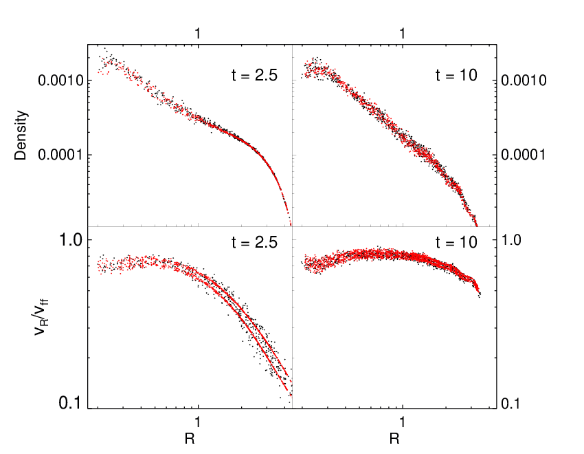
To compare the expected fluctuations given by equation 27 with those actually incurred, we ran a poorer resolution test with , i.e., ten times larger than the test shown in Figure 9. The errors (scatter) are then obviously larger. Figure 10 shows the results in black dots for two snapshots at times indicated. The red lines show the control run, as before, but this time velocity curves in the lower panel of the figure include the expected errors. In particular, the upper red sequence of dots is , whereas the lower red dots is , where is calculated with equation 27.
Evidently, the scatter in the radiation transfer simulation (black dots) is very similar in magnitude to what is predicted by equation 27. At the earlier time snapshot, shown on the left side of Figure 10, the measured velocity scatter is somewhat larger than our prediction. We believe this is due to the fact that equation 27 does not include the Poisson noise resulting from the initial distribution of photons packets at . The latter is generated by sampling a uniform random distribution in both emission time and directions.
In conclusion, these tests demonstrate the potential of the method for accretion and radiation pressure problems, and that equation 27 once again provides a reliable estimate of the stochastic errors of the results.
7 Discussion
A new method for implementation of radiation pressure force in an SPH code has been presented. Radiation is modelled via a time-dependent Monte-Carlo approach. Photon packet’s momentum is transferred to SPH particles via direct photon-to-gas interactions that are calculated as photons propagate through the field of SPH particles. The SPH density field is used to calculate the SPH density at photon packet’s positions, thus maximising the accuracy of the method. As a result, local and global momentum conservation in the interactions between radiation and gas is achieved.
Several tests have been presented to check the consistency and accuracy of the method, as well as error scalings with parameters of the problem. It was found that the main deficiency of the method, as for any Monte Carlo method, is the Poisson noise resulting from a finite number of photon packets used. In order to reduce velocity fluctuations to subsonic levels, photon packet’s momentum should be chosen to be below the typical SPH particle momentum, , where is the characteristic SPH particle velocity.
We shall now try to generalise and summarise the error estimates and various constraints on performance of the code.
7.1 Velocity errors
We first assume an optically thin case. Let be the radiation flux at a given location in the gas. The flux is related to the photon number density , photon momentum and photon velocity through
| (28) |
as the energy carried by the photon packet is . The rate at which photons are passing through SPH particles is
| (29) |
The momentum passed to the SPH particle by one photon packet is
| (30) |
and thus the velocity change is independent of SPH mass (in the optically thin approximation). Therefore, at time the velocity fluctuations can be estimated as
| (31) |
Now, let us define radiation acceleration time , where is the radiative acceleration acting on the SPH particle, and is the radiation pressure force on the SPH particle. During this characteristic time, the radiation pressure force would accelerate the SPH particle from rest to velocity in the absence of other forces.
Using equation 31, the Mach number of the fluctuations, defined by equation 22, can be shown to be
| (32) |
Finally, introducing the “optical depth” of the SPH particle as , we arrive at
| (33) |
where . This was derived in the optically thin limit, i.e., when . In the limit , the momentum passed from one photon to an SPH particle is reduced from the expression given by equation 30 to
| (34) |
where is the number of SPH neighbours for the photon. As the latter is always at least one when a photon packet interacts with gas, we arrive at the following estimate for the optically thick case,
| (35) |
Both the optically thin limit (equation 33) and the optically thick limit (equation 35) demonstrate the importance of choosing photon packet momentum, to be significantly smaller than that of an SPH particle to guarantee a reasonable accuracy.
We also notice that applicability of the method to a particular problem depends on the desired level of accuracy. For example, tidal disruption of a gaseous cloud near a luminous super-massive black hole is a highly dynamic process. To get an insight in the overall dynamics of the process, it is sufficient to simulate the system for a few dynamical times at the peri-centre of the orbit. A sufficiently small photon packet’s momentum, , should provide a sufficient accuracy in this case. However if one is interested in a secular evolution of a system, then the required precision is much higher, and careful tests should be done to establish the required value of , or equivalently the photon injection rate .
7.2 Number of photon packets
Let us now estimate the required number of photon packets for a given luminosity of the system , subject to the constraint , . Number of packets emitted per unit time is
| (36) |
where we exploited the fact that . here is the total gas mass of the system. The minimum time that the simulation should last for is the dynamical time, . During this time the number of photon packets emitted is , and thus
| (37) |
where is the radiation energy emitted during the system light crossing time and is the total gas energy. If there are no additional sources of radiation in the cloud, such as bright stars, then the luminosity of the system is of the order of where is the cooling time. In that case the ratio is
| (38) |
Many astrophysically interesting problems are in the regime where the cooling time is comparable with dynamical time of the system, in which case the ratio becomes
| (39) |
From these expressions it is obvious that the number of photons does not need to exceed the number of sph particles while satisfying the condition for these particular cases. However, if there is a very bright point source dominating the luminosity of the system, then the number of photon packets needs to be correspondingly higher. For example, in the tests presented in §5, photons produced during the duration of the simulations outnumbered SPH particles by factors of .
7.3 Optical depth of the system
Our radiation transfer method unfortunately becomes very expensive in optically thick medium, i.e., when the optical depth of the system, , is very high. This is due to two factors. First of all, photons scatter or get absorbed/re-emitted (that is many) times before they exit the system. They thus “hang around” for longer before exiting the system, hence increasing computational cost of the simulation. Secondly, they require smaller time steps as we now show.
Recall that in §2.5 we argued that it is numerically permissible and beneficial to use photon packets with velocity smaller than the velocity of light in the following case. In moderately optically thick, non relativistic plasmas, photons pass through the system much quicker than dynamical time, and hence exact value of is unimportant. The photon time step can then be increased inversely proportional to . However, this is possible only as long as
| (40) |
or else using too small a value for would incorrectly put the radiation transfer into the dynamic diffusion limit (see §2.5). Further, in the optically thick case the photon time step is limited to , where is the mean free path (equation 9). Comparing this to dynamical time of the system,
| (41) |
where we used equation 40 to constrain . This expression changes to
| (42) |
if one sets . Obviously, in both of these cases the time step becomes very small as increases, and the code becomes quite inefficient.
In problems with a very high optical depth combining the dynamic Monte Carlo and the diffusion approximation in very optically thick regions would be optimal, although it is not clear whether such “on the fly” method could be devised.
8 Conclusion
A new time-dependent algorithm to model radiation transfer in SPH simulations was presented. In the present paper we concentrated on the radiation pressure effects, i.e., the momentum transfer between the radiation and the gas, assuming a given equation of state for the gas. We performed a number of tests of the code.
Our method is grid-less and can be applied to arbitrary geometries. The main disadvantage of the method, as with any photon packet based schemes, is the Poisson noise due to a finite number of photons. On the other hand, these stochastic errors can be readily estimated and controlled by increasing the number of photon packets. The method is best applicable to optically thin or moderately optically thick systems, as following photon trajectories become very expensive at high optical depths.
Extension of the approach to include energy exchange between the gas and radiation will be presented in a future paper. Multi-frequency radiation transfer can also be naturally added.
9 Acknowledgments
The authors express gratitude to Volker Springel who provided the code Gadget-3, helped with the numerical implementation and provided useful comments on the paper. Theoretical astrophysics research at the University of Leicester is supported by a STFC Rolling grant.
References
- Altay et al. (2008) Altay G., Croft R. A. C., Pelupessy I., 2008, MNRAS, 386, 1931
- Baes (2008) Baes M., 2008, ArXiv e-prints, 809
- Benz (1990) Benz W., 1990, in Numerical Modelling of Nonlinear Stellar Pulsations Problems and Prospects, edited by J. R. Buchler, 269–+
- Brookshaw (1985) Brookshaw L., 1985, Proceedings of the Astronomical Society of Australia, 6, 207
- Clarke & Carswell (2003) Clarke C. J., Carswell R. F., 2003, Principles of Astrophysical Fluid Dynamics, Principles of Astrophysical Fluid Dynamics, by C. J. Clarke and R. F. Carswell, pp. 240. Cambridge University Press, 2003
- Dale & Bonnell (2008) Dale J. E., Bonnell I. A., 2008, MNRAS, 391, 2
- Dale et al. (2007) Dale J. E., Ercolano B., Clarke C. J., 2007, MNRAS, 382, 1759
- Fulk (1994) Fulk D. A., 1994, PhD thesis, Air Force Institute of Technology
- Garcia-Segura et al. (1996) Garcia-Segura G., Langer N., Mac Low M.-M., 1996, A&A, 316, 133
- Gingold & Monaghan (1977) Gingold R. A., Monaghan J. J., 1977, MNRAS, 181, 375
- Gritschneder et al. (2008) Gritschneder M., Naab T., Burkert A., Walch S., Heitsch F., Wetzstein M., 2008, ArXiv e-prints, 809
- Iliev et al. (2006) Iliev I. T., Ciardi B., Alvarez M. A., et al., 2006, MNRAS, 371, 1057
- Kessel-Deynet & Burkert (2000) Kessel-Deynet O., Burkert A., 2000, MNRAS, 315, 713
- Krumholz et al. (2007) Krumholz M. R., Klein R. I., McKee C. F., Bolstad J., 2007, ApJ, 667, 626
- Lamers & Cassinelli (1999) Lamers H. J. G. L. M., Cassinelli J. P., 1999, Introduction to Stellar Winds, Introduction to Stellar Winds, by Henny J. G. L. M. Lamers and Joseph P. Cassinelli, pp. 452. ISBN 0521593980. Cambridge, UK: Cambridge University Press, June 1999.
- Lucy (1977) Lucy L. B., 1977, AJ, 82, 1013
- Lucy (1999) Lucy L. B., 1999, A&A, 344, 282
- Monaghan (1992) Monaghan J. J., 1992, ARA&A, 30, 543
- Oxley & Woolfson (2003) Oxley S., Woolfson M. M., 2003, MNRAS, 343, 900
- Pawlik & Schaye (2008) Pawlik A. H., Schaye J., 2008, ArXiv e-prints, 802
- Petkova & Springel (2008) Petkova M., Springel V., 2008, ArXiv e-prints
- Price (2004) Price D., 2004, PhD thesis, University of Cambridge
- Ritzerveld & Icke (2006) Ritzerveld J., Icke V., 2006, Physical Review E, 74, 2, 026704
- Rybicki & Lightman (1986) Rybicki G. B., Lightman A. P., 1986, Radiative Processes in Astrophysics, Radiative Processes in Astrophysics, by George B. Rybicki, Alan P. Lightman, pp. 400. ISBN 0-471-82759-2. Wiley-VCH , June 1986.
- Shakura & Sunyaev (1973) Shakura N. I., Sunyaev R. A., 1973, A&A, 24, 337
- Springel (2005) Springel V., 2005, MNRAS, 364, 1105
- Stamatellos & Whitworth (2005) Stamatellos D., Whitworth A. P., 2005, A&A, 439, 153
- Susa (2006) Susa H., 2006, PASJ, 58, 445
- Viau et al. (2006) Viau S., Bastien P., Cha S.-H., 2006, ApJ, 639, 559
- Vishniac (1983) Vishniac E. T., 1983, ApJ, 274, 152
- Whitehouse & Bate (2004) Whitehouse S. C., Bate M. R., 2004, MNRAS, 353, 1078
- Whitehouse & Bate (2006) Whitehouse S. C., Bate M. R., 2006, MNRAS, 367, 32
- Whitehouse et al. (2005) Whitehouse S. C., Bate M. R., Monaghan J. J., 2005, MNRAS, 364, 1367