Sparse Network Coding with Overlapping ClassesThanks: ¹ Supported by CAPES Foundation, Brazil.

Network coding [1, 2, 3, 4, 5] is a promising approach to data dissemination over networks. In this past decade, several works have attempted to establish the potential of this simple and yet seemingly revolutionary idea in a variety of applications [6, 7, 8, 9, 10, 11]. While the success of network coding for streaming media and wireless applications has been encouraging, it is still unclear whether this approach is beneficial for peer-to-peer file dissemination [12]. The present paper is an initial attempt to fill this gap.

One major issue is decoding complexity. In the file-downloading scenario, a large file of $km\log_{2}q$ bits is to be distributed among cooperating peers in a network. The file is partitioned into $k$ packets, each consisting of $m$ symbols over a finite field $\mathbb{F}_{q}$. If random linear network coding [4] is used to distribute the file, then each receiver has to solve a linear system with $k$ equations in order to decode the file. This requires $O(k^{3}+k^{2}m)$ operations in $\mathbb{F}_{q}$, which may be prohibitively expensive in practice.

To reduce the decoding complexity, Chou et al. [5] proposed to group packets into disjoint generations, each containing $d$ packets, and apply network coding only within each generation. The complexity issue is solved if $d$ is small, but another problem is created: that of efficiently routing $L=k/d$ generations throughout the network.

Note that simply choosing a small $k$ and compensating the file size by using a large packet length $m$, as done in [7], may not be a satisfactory solution. Transmitting such large packets (of, say, 1–4 MBytes [7]) over a dynamic peer-to-peer network—where peers may interrupt transmissions or leave the network at any time—is a highly nontrivial problem. Since each coded packet is essentially unique, interrupted transmissions are useless to a receiving peer, potentially causing a severe waste of bandwidth. Thus, we find it more realistic to assume that $m$ is small and $L$ is large.

Probably the most successful approach so far to routing pieces of a file through a peer-to-peer network is the BitTorrent protocol [13]. The drawback of this and similar protocols is that a large number of control messages must be exchanged between peers, mainly to resolve the problems of rare blocks and block reconciliation [14, 15]. Thus, the protocol overhead is substantial, and a significant amount of research has been devoted to trying to alleviate this problem [14].

The solution proposed by Maymounkov et al. [16], in the context of generation-based network coding, completely eliminates any protocol overhead: peers randomly choose the generation from which to transmit each packet. This scheme is called chunked coding. Intuitively, the scheme replaces protocol overhead with transmission overhead. While the scheme is shown to have a good performance asymptotically, the performance quickly deteriorates for practical values of $d$.

A related line of work is fountain coding [17]. By using optimized degree distributions, fountain codes such as LT or raptor codes can achieve a relatively small overhead with a low-complexity back-substitution decoder [17]. These schemes, however, are not compatible with network coding. To maintain the designed degree distributions, packets must travel intact throughout the network—otherwise, the decoder would fail miserably.

This paper investigates the following question: is it possible to use a true network coding approach and yet enjoy a low-complexity fountain-like decoder? The approach proposed here answers this question affirmatively, and can be seen as a combination of fountain coding and network coding. Our idea is to follow the approach of chunked coding, but instead use a larger number of overlapping generations (here called classes). Overlapping generations allow packets from decoded generations to be back-substituted into still undecoded generations, in the same spirit of a fountain decoder. This not only boosts the performance but also reduces the decoding complexity of the scheme.

The remainder of the paper is organized as follows. In Section II, we review previous work on network coding in a way that simplifies the description of our codes and emphasizes the existing connections. Section III presents our approach, including the description of the decoder and bounds on the decoding complexity. In Section IV, we present some code constructions, whose performance is evaluated in Section V and compared with that of chunked codes. Finally, Section VI presents some concluding remarks.

In this section we present a novel scheme that attempts to overcome the drawbacks of chunked coding. From one perspective, the scheme can be seen as a fountain code that is fully compatible with network coding.

In the following, the term class refers to a non-empty subset of $\{1,\ldots,k\}$. A class-based scheme for network coding is specified by a set of classes, $\mathcal{C}=\{C_{1},\ldots,C_{L}\}$, and a probability distribution on classes, $\{p_{1},\ldots,p_{L}\}$. When $\mathcal{C}$ is understood, we may write class $\ell$ as a shorthand for class $C_{\ell}$. Let $\supp(g)$ be the support of a vector $g\in\mathbb{F}_{q}^{k}$, i.e., $\supp(g)=\{i\in\{1,\ldots,k\}\colon{g_{i}\neq 0}\}$. For a packet $x\in\mathbb{F}_{q}^{m}$ with coding vector $g\in\mathbb{F}_{q}^{k}$, we say that $x$ belongs to class $\ell$ if $\supp(g)\subseteq C_{\ell}$. Let $\lambda(x)$ denote the set of indices of all the classes to which a packet $x$ belongs, i.e., $\lambda(x)\triangleq\{\ell\in\{1,\ldots,L\}\colon\supp(g)\subseteq C_{\ell}\}$. With a slight abuse of terminology, we will usually refer to a class $\ell$ to mean all the data packets belonging to that class.

Note that, in general, a packet $u_{i}$ may belong to multiple classes; for instance, we might have $C_{1}\cap C_{2}=\{i\}$, which implies that $\{1,2\}\subset\lambda(u_{i})$. When two classes have non-empty intersection, we will say that these classes overlap.

Given a class-based network coding scheme $(\mathcal{C},\{p_{\ell}\})$, every node in the network (including the source node) performs, at each transmission opportunity, the following encoding procedure. First, a class index $\ell$ is randomly selected according to $\{p_{\ell}\}$. If no packets from that class have yet been received, then the process is repeated until an index $\ell$ is selected such that some packet from class $\ell$ has been received. Then, an outgoing packet is computed as a random linear combination of received packets from class $\ell$.

Let $d_{\ell}=|C_{\ell}|$, for $\ell=1,\ldots,L$. It should be clear that the chunked coding scheme described in Section II-B corresponds to the special case where $\mathcal{C}$ is a partition of $\{1,\ldots,k\}$, with $d_{\ell}=d=k/L$, and $\{p_{\ell}\}$ is uniform. In general, due to the presence of overlapping classes, we may have $\sum_{\ell=1}^{L}d_{\ell}>k$.

Let us now describe the decoding process. For $\ell=1,\ldots,L$, let $Y^{(\ell)}$ consist of the received packets from class $\ell$, and let $r_{\ell}=\rank Y^{(\ell)}$. We view $Y^{(\ell)}$, and therefore $r_{\ell}$, as variables that are constantly updated as new packets are received; in particular, we call the tuple $(r_{1},\ldots,r_{L})$ the state of the receiver. In the context of a decoding process, we say that a class $\ell$ is decodable if $r_{\ell}\geq d_{\ell}$ and that it has been decoded if all the data packets $u_{i}$ belonging to $\ell$ have been recovered. Decoding starts from some decodable class $\ell$ that has not yet been decoded. This class is decoded by Gaussian elimination. Then, similarly to the decoding of fountain codes, any data packets $u_{i}$ belonging to $C_{\ell}$ are back-substituted into any overlapping classes, and the ranks $r_{1},\ldots,r_{\ell}$ are recomputed. For instance, if $u_{i}$ belongs to classes $1$ and $2$, and class $1$ is decoded, then we may imagine that a new packet $y^{(2)}_{n_{2}+1}=u_{i}$ has been received. Unless class $2$ has already been decoded, this has the effect of increasing $r_{2}$ by one unit. The process is then repeated until all classes have been decoded—which is to say that all data packets $u_{i}$ have been obtained.

The essence of the decoding process is similar to solving a crossword puzzle: when a word is “decoded,” the recovered letters can be reused to help in the decoding of any overlapping words. Indeed, the idea of a crossword puzzle gives the basis for the simplest nontrivial overlapping scheme, which we call grid codes. A simple example of a grid code is given in Fig. 1b.

A general definition will be presented in Section IV.

Let us now examine the issue of decoding complexity. We first describe an alternative way to view the decoding process. Note that, for each new packet $u_{i}$ that is recovered, one variable is effectively removed from the problem for all the remaining classes. Thus, rather than increasing $r_{1},\ldots,r_{L}$ at each decoding iteration, we can equivalently decrease $d_{1},\ldots,d_{L}$. This has precisely the same effect in the decoding condition $r_{\ell}\geq d_{\ell}$. More precisely, let $d_{\ell}^{(i)}$ denote the size of class $\ell$ (in terms of remaining variables) after the $i$th decoding iteration. Initially, $d_{\ell}^{(0)}=d_{\ell}$, for all $\ell$. After the $i$th iteration, when, say, class $\ell^{*}$ is decoded, we update $d_{\ell}^{(i)}=d_{\ell}^{(i-1)}-|C_{\ell}\cap C_{\ell^{*}}|$, for all classes that have not yet been decoded. We keep $d_{\ell}^{(i)}=d_{\ell}^{(i-1)}$ for the decoded classes, since this tells us precisely the size of the problem that was solved for class $\ell$, i.e., how many packets had to be decoded by Gaussian elimination. Thus, at the end of the decoding process, say, after iteration $t$, we should have $\sum_{\ell=1}^{L}d_{\ell}^{(t)}=k$, which is precisely the total number of variables. Using this description of the decoding process, we can provide the following bound on the decoding complexity.

In this section, we present some examples of codes with overlapping classes. The performance of these codes will be investigated in Section V.

Note that, in a $d^{\prime}\times d$ grid code, the first $d^{\prime}$ classes have size $d$ and form a partition of $\{1,\ldots,k\}$, while the last $d$ classes have size $d^{\prime}$ and also form a partition of $\{1,\ldots,k\}$.

When all classes have the same size, i.e., $d^{\prime}=d$, we obtain square grid codes. These codes are, unfortunately, too restrictive, since we must have $k=d^{2}$. A way to span a higher number of packets with fixed-size classes is provided by diagonal grid codes. For convenience, in the next definitions, assume that packet and class indices are numbered starting at zero.

For $s=0,\ldots,\lceil L/L_{0}\rceil-1$, the classes $C_{sL_{0}}$,$\ldots$,$C_{(s+1)L_{0}-1}$ form a partition of $\{0,\ldots,k-1\}$. In particular, the $L_{0}$ classes with angle $\theta_{s}=0$ correspond to a chunked code. An example of a diagonal grid code is given in Fig. 3.

The design of a diagonal grid code minimizes the maximum size of the intersection of two classes. It is easy to see that, if all the nonzero $\theta_{s}$ are relatively prime to $L_{0}$, then any two distinct classes overlap in at least $\lfloor L/L_{0}\rfloor-1$ and at most $\lceil L/L_{0}\rceil-1$ classes. To see that this value is optimal, consider a bipartite graph with packets and classes as nodes, and an edge connecting a packet to a class if that packet belongs to that class. It follows that the maximum degree of a packet must be at least the average degree $(Ld)/(L_{0}d)=L/L_{0}$.

Note that a diagonal grid code consists essentially of multiple layers of chunked codes each applied after the packets $0,\ldots,k-1$ undergo a certain (grid-like) permutation. Thus, the construction of Definition 2 can be generalized by using arbitrary permutations. For $s=0,\ldots,\lceil L/L_{0}\rceil-1$, let $\pi_{s}$ be a permutation of $\{0,\ldots,k-1\}$. Then we may consider a code with $L$ classes of size $d$ given by

where $L_{0}=k/d$. Without loss of generality, we will assume that $\pi_{0}$ is the identity permutation. If all the remaining permutations are chosen uniformly at random, we will call the resulting code a random-layer code.

For generality, in all the codes described above, we have left the probability distribution $\{p_{\ell}\}$ unspecified. However, in the case that all classes have a constant size $d$, it is quite natural to use a uniform distribution $p_{\ell}=1/L$ for all $\ell$. More generally, we see no reason to assign different probabilities for classes of the same size, and we will use this assumption in all the experiments in the next section.

In this section, we use simulations to evaluate the performance of the codes described in the previous section.

We make the following assumptions:

1. 1.

   All received packets are linearly independent whenever possible, i.e., $\rank A^{(\ell)}B^{(\ell)}=\min\{n_{\ell},d_{\ell}\}$, for all $\ell$.

2. 2.

   The probability that a received packet belongs to class $\ell$ is exactly equal to $p_{\ell}$, for all $\ell$.

Note the two assumptions above concern themselves with the network topology and the network code, and they are required if we wish to pursue an analysis that is independent of the network. Assumption 1 implies that the source node must generate a sufficient number of packets from each class ($N_{\ell}\geq d_{\ell}$) and that both the encoding at the source node and the network code must not introduce any linear dependence on any set of up to $d_{\ell}$ received packets. Assumption 2 means that the network preserves the designed probability distribution on classes. Both assumptions should hold true if $q$ and each $d_{\ell}$ are sufficiently large. In order to satisfy this requirement, we assume that a parameter $d_{\min}$ is given such that any valid code must satisfy $d_{\ell}\geq d_{\min}$, for all $\ell$. Specifically, we consider $d_{\min}=25$ in the following results. Note that the value of $q$ does not affect code design.

Performance is evaluated in terms of the complexity-overhead tradeoff. Since the problem is inherently delay-tolerant—each receiver is interested in receiving the complete file with probability 1, no matter how long it takes—the two main figures of merit are the expected complexity and the expected overhead. Note that the figure of expected overhead automatically incorporates the probability of failure for each specific overhead, therefore eliminating the need to consider a three-dimensional tradeoff space.

Fig. 4 shows how complexity is traded off against overhead in a chunked coded.

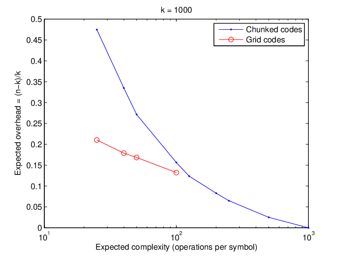
At one extreme, we have a dense code with a single class of size $d=k$; this code has optimal overhead but prohibitively large complexity. At the other extreme we have a chunked code with class size $d=d_{\min}$, which attains the minimum possible complexity at the expense of a large overhead. As shown in Fig. 4, for small to moderate complexity, diagonal grid codes can outperform chunked codes by a large margin. Note that the complexity of diagonal grid codes is precisely equal to the class size $d$. The number of classes $L$ for each grid code has been tuned experimentally to maximize the performance for the given parameters. From left to right, the points in Fig. 4 correspond to $L=28$, $12$, $9$, $2$.

Fig 5 shows similar results for a scenario where $k=4096$. As one can see, well-designed grid codes significantly outperform chunked codes. From left to right, the grid codes in the figure have $L=207$, $92$, $43$. Fig 5 also shows the performance of codes with varying class sizes, referred to as mixed codes.

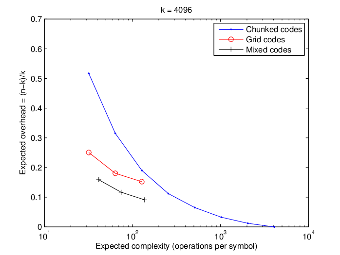
From left to right, these codes are: a $(4096,32,200)$ diagonal grid code with an additional random class of size 2048; a $(4096,64,86)$ diagonal grid code with an additional random class of size 1024; and a $(4096,128,38)$ diagonal grid code with an additional random class of size 512. In all cases, the distribution $\{p_{\ell}\}$ used is the uniform one. In comparison with their corresponding grid codes, the mixed codes exhibit a significantly lower overhead with only a marginal increase in complexity. As discussed in Section III, this is due to the fact that the extra (large) class is typically decoded only after many other (smaller) classes have been decoded and back-substituted. The effect of a large class is analogous to that of a high degree check in LT codes: establishing a “bridge” between non-overlapping classes and thus allowing the decoding “ripple” [17] to be maintained for a longer time.

Our results show that, for a fixed expected complexity, the use of overlapping classes can reduce the expected overhead by up to 70%.

This paper presents a novel approach to network coding based on the concept of overlapping classes. The approach generalizes chunked coding and allows a propagative decoder that enjoys many of the benefits of fountain codes. Our proposed scheme, while still in its initial stages, seems to be a promising step towards a full network coding solution to peer-to-peer file distribution. More generally, our approach seems to be suitable for any application that would benefit from a combination of fountain coding and network coding.

We remark that, while our analysis assumes no feedback between nodes, nothing prevents a protocol based on our scheme from using control messages to aid the communication. By carefully designing the amount of protocol overhead, the overall performance of the scheme may be further increased.

Our main objective with this paper has been to suggest a new possible direction for research in network coding, as more questions remain open than have been answered here (especially in the theoretical side). In particular, the design of good codes with constant or non-constant class sizes (and possibly nonuniform distribution) is an important open problem. Due to the recursive nature of the decoding process, the development of analytical bounds on performance also remains elusive at this point. We hope to address both problems in our future work.

References

- [1] R. Ahlswede, N. Cai, S.-Y. R. Li, and R. W. Yeung, “Network information flow,” IEEE Trans. Inf. Theory, vol. 46, no. 4, pp. 1204–1216, Jul. 2000.
- [2] S.-Y. R. Li, R. W. Yeung, and N. Cai, “Linear network coding,” IEEE Trans. Inf. Theory, vol. 49, no. 2, pp. 371–381, Feb. 2003.
- [3] R. Koetter and M. Médard, “An algebraic approach to network coding,” IEEE/ACM Trans. Netw., vol. 11, no. 5, pp. 782–795, Oct. 2003.
- [4] T. Ho, M. Médard, R. Koetter, D. R. Karger, M. Effros, J. Shi, and B. Leong, “A random linear network coding approach to multicast,” IEEE Trans. Inf. Theory, vol. 52, no. 10, pp. 4413–4430, Oct. 2006.
- [5] P. A. Chou, Y. Wu, and K. Jain, “Practical network coding,” in Proc. Allerton Conf. on Comm., Control, and Computing, Monticello, IL, Oct. 2003, pp. 40–49.
- [6] C. Gkantsidis and P. Rodriguez, “Network coding for large scale content distribution,” in Proc. 24th IEEE Int. Conf. on Computer Commun., Mar. 13–17, 2005, pp. 2235–2245.
- [7] C. Gkantsidis, J. Miller, and P. Rodriguez, “Comprehensive view of a live network coding p2p system,” in Proc. ACM Internet Measurement Conf., Rio de Janeiro, Brazil, Oct. 25–27, 2006.
- [8] S. Katti, H. Rahul, W. Hu, D. Katabi, M. Medard, and J. Crowcroft, “XORs in the air: Practical wireless network coding,” IEEE/ACM Trans. Netw., vol. 16, no. 3, pp. 497–510, Jun. 2008.
- [9] C. Fragouli, J. Widmer, and J.-Y. Le Boudec, “Efficient broadcasting using network coding,” IEEE/ACM Trans. Netw., vol. 16, no. 2, pp. 450–463, Apr. 2008.
- [10] M. Wang and B. Li, “: Random push with random network coding in live peer-to-peer streaming,” IEEE J. Sel. Areas Commun., vol. 25, no. 9, pp. 1655–1666, 2007.
- [11] A. Dimakis, P. Godfrey, M. Wainwright, and K. Ramchandran, “Network coding for distributed storage systems,” in Proc. 26th IEEE Int. Conf. on Computer Commun., Anchorage, AK, May 6–12, 2007, pp. 2000–2008.
- [12] D. M. Chiu, R. W. Yeung, J. Huang, and B. Fan, “Can network coding help in P2P networks?” in Proc. NetCod, Apr. 2006.
- [13] B. Cohen, “The BitTorrent protocol specification.” [Online]. Available: http://www.bittorrent.org
- [14] A. R. Bharambe, C. Herley, and V. N. Padmanabhan, “Analyzing and improving a BitTorrent network’s performance mechanisms,” in Proc. 25th IEEE Int. Conf. on Computer Commun., Barcelona, Spain, Apr. 2006.
- [15] J. Xu, J. Zhao, X. Wang, and X. Xue, “Swifter: Chunked network coding for peer-to-peer content distribution,” in Proc. IEEE Int. Conf. on Commun., May 19–23, 2008, pp. 5603–5608.
- [16] P. Maymounkov, N. J. A. Harvey, and D. S. Lun, “Methods for efficient network coding,” in Proc. Allerton Conf. on Comm., Control, and Computing, Monticello, IL, Sep. 2006, pp. 482–491.
- [17] A. Shokrollahi, “Raptor codes,” IEEE Trans. Inf. Theory, vol. 52, no. 6, pp. 2551–2567, Jun. 2006.