We introduce a general way of modeling inflation in a framework that is independent of the exact nature of the inflationary potential. Because of the choice of our initial conditions and the continuity of the scale factor in its first two derivatives, we obtain non-divergent results without the need of any renormalization beyond what is required in Minkowski space. In particular, we assume asymptotically flat initial and final values of our scale factor that lead to an unambiguous measure of the number of particles created versus frequency. We find exact solutions to the evolution equation for inflaton perturbations when their effective mass is zero and approximate solutions when their effective mass is non-zero. We obtain results for the scale invariance of the inflaton spectrum and the size of density perturbations. Finally, we show that a substantial contribution to reheating occurs due to gravitational particle production during the exit from the inflationary stage of the universe.

The second part of this dissertation deals with a post-Minkowski approximation to a binary point mass system with helical symmetry. Numerical solutions for particles of unequal masses are examined in detail for two types of Fokker actions, and these solutions are compared with predictions from the full theory of General Relativity and with post-Newtonian approximations. Analytic solutions are derived for the Extreme Mass Ratio case.

The third part of this dissertation discusses the detection sensitivity of the IceCube Neutrino Telescope for observing interactions involving TeV-scale black holes produced by an incoming high-energy cosmic neutrino colliding with a parton in the Antarctic ice of the south pole. Parton Distribution Functions and the black hole interaction cross section are computed numerically. Our computation shows that IceCube could detect such black hole events at the 5-sigma level for a ten-dimensional Planck mass of 1.3 TeV.

Major Professor Date

ACKNOWLEDGMENTS

I wish to thank my advisor, Distinguished Professor Leonard Parker, for suggesting Part I of this dissertation. I appreciate his patience, his trust, and his guidance. Without his pioneering work on gravitational particle production, this dissertation would not have been possible.

I am also thankful for my other collaborators on Parts II and III, Kōji Uryū and Luis Anchordoqui. Kōji graciously let me contribute to his research, even though he could have calculated my results faster by himself. I appreciate Luis’s generosity and his sincere desire to see me succeed in physics and life.

I am grateful for the support of the Lynde and Harry Bradley Foundation, and for the support of the National Space Grant College and Fellowship Program and the Wisconsin Space Grant Consortium.

My wife, Alyson, sacrificed her own scholarships so that I might attend the University of Wisconsin—Milwaukee. Thank you.

Chapter 1 Introduction

This dissertation is an exploration of space on scales that are small (quantum fluctuations, TeV-scale black holes, vacuum particle creation); scales that are big (anisotropies in the Cosmic Microwave Background, seeding of large-scale structure, the Hubble radius); and scales that are in between (Extreme Mass Ratio binary black holes, temperatures associated with horizons, Innermost Stable Circular Orbits). The first part of this dissertation is an outgrowth of methods developed by my thesis advisor in the following works [1, 2, 3, 4]. These methods are applicable to the creation of quantized perturbations of the inflaton field, which is the topic we explore in Part I. The new results that appear in this dissertation are based primarily on the work of three papers. The first of these papers, “Study of the Spectrum of Inflaton Perturbations,” examines an exact calculation of the evolution of quantum fluctuations and the subsequent particle creation in a model of the early expansion of the universe that is relevant to a wide range of inflationary potentials consistent with observations and that does not depend on renormalization in curved spacetime [5]. The second of these papers, “Circular solution of two unequal mass particles in Post-Minkowski approximation,” computes numerically a set of solutions to a helically symmetric binary system of point masses in a particular approximation to General Relativity and presents analytical formulas for the limit that the mass of the lighter particle is negligible with respect to that of the more massive particle [6]. The third of these papers, “Black Holes at the IceCube neutrino telescope,” calculates the experimental sensitivity for observing TeV-scale black holes produced by a gravitational interaction between a cosmic neutrino and an elementary particle within the atomic nuclei of ice molecules [7]. This dissertation is divided into three main parts corresponding to these three papers.

In Part I, “New Aspects of Inflaton Fluctuations,” we begin with a brief summary of early universe cosmology. Two of the most important cosmological theories of the twentieth century are the Big Bang theory and the theory of Inflation. The Big Bang theory supposes that our universe was once much smaller and much hotter that it is today. It explains the expansion of the universe, the presence of the Cosmic Microwave Background Radiation, and the primordial abundances of light elements. Cosmological Inflation supposes that the early universe underwent an extremely large increase in size in a very small amount of time. This explains why the density of our universe today is so close to the critical density that separates a universe that expands forever from one that eventually recollapses, it explains the near homogeneity and isotropy of the universe, and it explains why we don’t observe magnetic monopoles. Most importantly of all, however, inflation explains the origins of those anisotrophies that do exist in our universe. Although a key ingredient of the Big Bang theory is a high energy density in the early universe and a correspondingly high temperature, the classical theory of inflation predicts an extreme cooling of the universe as it expands— much like the air in a piston cools as it expands to do work on its surroundings. We consider Reheating, and specifically the energy density of particles created by an expanding universe, as a means of preserving both theories without sacrificing any of their successes. We give a general overview of the amplification of quantum fluctuations into large-scale density perturbations during inflation, and we describe some of the ways of relating theoretical predictions to observations. We then list some of the observational findings of experiments.

We continue with the details of the method we use to model inflation. Instead of specifying an inflationary potential, as is usually done, we specify directly the change in the scale factor, which is a measure of the size of the universe, versus time. We consider a scale factor that accommodates several parameters, but its most important features are that it asymptotically approaches a constant values at early times, that it approaches a different constant value at late times, and that its first two derivatives with respect to time are continuous. The asymptotically flat regions of our scale factor allow us to associate our model with Minkowski spacetime at early and late times. Identification with a Minkowski vacuum at early times leads us to initial conditions that contain no infrared divergences, and comparison with a Minkowski spacetime at late times leads us to an unambiguous measure of the frequency-dependent density of particles created by the expansion of the universe. That our scale factor is continuous up to its second derivative with respect to time ensures we have no ultraviolet divergences, in addition to the prevention of infrared divergencies mentioned before. We choose for our scale factor a composite of three segments. The initial and final segments are each associated with a particular form of asymptotically flat scale factor with different choices of parameters. The middle segment of the scale factor, where most of the expansion takes place, is a region that grows exponentially with respect to proper time. Such an exponential growth is indicated by experimental observations. We solve for the matching conditions necessary to maintain the desired continuity of our composite scale factor. For each of our scale factor segments we have exact solution to the evolution equation for fluctuations of a massless, minimally-coupled scalar field. We also describe two different approximations to the case of a constant mass. We match up our solutions to the evolution equation at the interfaces between the segments of our composite scale factor, and at late times we are able to determine the particle production due to the expansion of the universe. From here we discuss the dispersion spectrum. We note the scale-invariance of the scalar index, provided the requirement is met that each mode be converted into a curvature perturbation at a time related to when it crosses the Hubble radius, and that all modes not be converted at once after the end of inflation. Using a hybrid combination of our method with the slow roll approximation, we describe a way of calculating the density perturbations produced by inflation. Finally, we show how Reheating, or a return to the hot Big Bang conditions after the end of inflation, can accompany inflation. We discuss possible consequences of Reheating and its relationship to constraints on predictions for exotic particles and high energy physics.

In Part II, “Binary System of Compact Masses,” we examine a post-Minkowski approximation to a helically symmetric binary system of point masses. The helical symmetry is maintained through the presence of half-advanced and half-retarded fields. The equations of motion are given for one of two Fokker actions— parametrization-invariant and affine— by Friedman and Uryū in [8], and from their results we calculate numerically the solutions in the case of unequal masses. We also derive analytical formulas for the Extreme Mass Ratio limit where the ratio of the smaller mass divided by the larger mass goes to zero. This limit would be applicable to the inspiral of a solar-mass black hole into a billion-solar-mass black hole, such as is predicted to exist at the centers of many galaxies. For both the numerical computations and the analytic equations, we plot three graphs: the angular momentum versus the velocity of the lighter particle, the unit energy of the lighter particle versus the angular momentum, and the unit angular momentum of the lighter particle versus the angular momentum. These plots are given for four mass ratios and for both types of Fokker action. For the parametrization-invariant case we include one of two different correction terms that generates solutions that agree with the first post-Newtonian approximation, and we demonstrate this in the Extreme Mass Ratio limit. We discuss the locations of Innermost Stable Circular Orbits, and we compare the predictions of this post-Minkowski approximation with both those of the post-Newtonian approximation and those of the full theory of General Relativity.

In Part III, “Production and Decay of Small Black Holes at the TeV-Scale,” we investigate the possibility of using the IceCube Neutrino Telescope to detect TeV-scale black holes. In the physics of the Standard Model, it is not impossible that a cosmic neutrino could come close enough to an elementary particle in the cubic kilometer of ice in the IceCube experiment to form a black hole. Such interactions involving gravity, however, are so much less likely than interactions involving the weak force, that IceCube would never differentiate their signal from the background noise of weak-interaction event rates. Many theories of physics beyond the Standard Model, such as string theory, require additional dimensions of spacetime beyond the 3+1 dimensions of our common experience. These additional dimensions might not have been noticed before if they were compactified, or curled up, with a simple example being the topology of a higher-dimensional torus. At the compactification scales, then, gravity would be much stronger than in a 3+1-dimensional theory, whereas at macroscopic scales gravity would appear to be much weaker than the strong and electroweak forces. In addition, if only gravitons propagated into the compactified dimensions, then the scale of compactification could be anything small enough not to conflict with observations. On distances smaller than this scale, gravity would grow stronger with decreasing separation faster than an inverse-square law would predict. If the strength of gravity were equal to the strength of the electromagnetic force around energies of roughly one TeV, or $10^{-19}$ meters, the scale at which the electromagnetic and weak forces unify into the electroweak force, then gravity could be sufficiently strong that the IceCube detector could observe the production of TeV-scale black holes in the interactions between cosmic neutrinos and partons, which are the fundamental particles— both quarks and gluons— that are found within nucleons in atoms. For the high energies of interest for this experiment, the nucleons cannot be treated as single particles, which is why we treat them as collections of partons. At any moment, a parton can have an energy ranging from nothing to the entire rest mass energy of the nucleon, and parton distribution functions describe the probabilities of finding each parton with a given energy. We develop simple fits to a specific model of the parton distribution function, and with this information we are able to numerically integrate an expression giving us the cross section for the gravitational interaction. The black holes formed by these interactions would decay almost immediately via Hawking radiation, or particles produced by the strong curvature of spacetime outside of black holes. The Cherenkov light of these events could be measured by the photomultiplier tubes of IceCube, and signals could be picked out from the background event rate by searching for muon-daughter particles with less than 20% of the total energy, which is sufficiently unlikely in Standard Model physics that we would be able to discern TeV-scale black hole events from interactions through the weak force. We find that the IceCube detector could measure TeV-scale black holes at a statistically significant 5 $\sigma$ excess for a 10-dimensional Planck scale of 1.3 TeV.

The relationship between space at the smallest and largest scales is, perhaps, nowhere so evident as the inflation of quantum fluctuations from below the Planck length to sizes beyond our observable universe in what follows: Part I - New Aspects of Inflaton Fluctuations.

Part I:

New Aspects of

Inflaton Fluctuations

Chapter 2 Inflationary Cosmology

At the beginning of the twentieth century, most scientists believed that the universe was infinite and eternal. Such a situation is not compatible with cosmology governed by the theory of General Relativity, which predicts that a static universe would be unstable to perturbations. From this it follows that our expanding universe started from a singularity of infinite density and temperature. This Big Bang theory of the universe successfully explains several observational phenomena. One of these is the expansion of the universe and Olber’s paradox, which asks— if the universe is infinite, then why do we not observe stars in every direction; why do we see dark space between stars? With help from Hubble, Einstein and others came to realize that the universe is not only expanding, but it must also have a finite age. Thus, not all of the light from stars in the universe has had time to reach us, and for distant stars this light is redshifted by the expansion of the universe. Another question resolved by the Big Bang theory is that of the primordial abundances of the light elements: hydrogen, deuterium, tritium, helium-3, helium-4, and lithium. Stars convert hydrogen to heavier elements through nuclear fusion, but the light elements are found in definite ratios in galactic dust thought never to have been part of any star. This is explained by looking back to the high temperatures and pressures of the universe when it was much more dense, shortly after the Big Bang. The universe was hotter than any star, and a series of calculations involving the thermal-equilibrium ratio of protons to neutrons, the ratio of baryons to photons, the half-life for a free neutron, and the cross section for neutrons to become bound in nuclei [9, 10]; predicts ratios of primordial abundances of the light elements that agree very well with observations. A final success of the Big Bang theory is the explanation of the observed Cosmic Microwave Background Radiation (CMBR) at a temperature of approximately 2.7 Kelvin. This was first discovered by Penzias and Wilson in 1965 while they were working at Bell Labs, and for this discovery they were awarded a Nobel Prize in 1978. This background noise is the red-shifted relic of the early universe’s radiation dominance. Although the Big Bang theory explained some questions about our universe, Cosmological Inflation was necessary to explain other observed properties of our universe.

Inflation was originally conceived to explain three primary phenomena. The first of these was the flatness problem. The density of our universe is surprisingly close to the critical density needed to close the universe, above which a closed universe would eventually re-collapse into a Big Crunch and below which an open universe would expand forever— neglecting acceleration caused by the presence of dark energy. Surprisingly close, because unless our universe’s density is precisely equal to the critical density— and there is no reason to assume it must be— the ratio between the two drifts rapidly away from 1 in a Big-Bang-only universe. Inflation solves this problem by very rapidly driving this ratio exceedingly close to 1 during a short period of enormous growth of the universe. The second argument for inflation is that all the CMBR is, to excellent approximation of within about one part in ten thousand, in thermal equilibrium. Just as the resolution to Olber’s paradox involves light taking a finite time to reach the Earth, so does this present a problem for early-universe light, emanating from different directions, that is just now reaching us. In a Big-Bang-only model, widely separated regions of the currently observable universe weren’t previously in causal contact, and that they should be in thermal equilibrium now is a mystery. This problem is resolved by explaining how the space in minute regions of our universe that were once in thermal contact expanded sufficiently rapidly during inflation to remove the different parts of the equilibrated sections to causally disconnected parts of the universe: the space between points within equilibrated regions of the universe grew much faster than signals could travel across the distance between those points. Thus, the CMBR reaching the Earth today, even from different directions, has come from regions of the universe that were previously in thermal equilibrium. The third issue that motivated inflation is the observed absence of magnetic monopoles, which may have been created in the very early universe. Inflation resolves this by showing how monopoles could be inflated away with the expansion of space such that— unless monopoles were produced after inflation— on average there shouldn’t be any monopole close enough to us to detect after inflation.

Inflation has come up with an unforseen prediction that has since turned out to be more important than any of the historical justifications for its existence: the creation of fluctuations during inflation that lead to the anisotropies of our present-day universe. For NASA-COBE’s (Cosmic Background Explorer) 1989 detection of these anisotropies in the CMBR, Mather and Smoot were awarded a Nobel Prize in 2006. In the most widely used models of inflation, this expansion is driven by the inflaton field, which is a scalar quantum field, and the perturbations of the inflaton field seed galaxy formation and are responsible for large-scale structure of our universe today.

2.1 Cosmology in General Relativity

In units of $c=\hbar=1$ Einstein’s equation is [11, 12]

G_{ab}\equiv R_{ab}-\frac{1}{2}Rg_{ab}=8\pi G\,T_{ab}.

(2.1)

On large enough scales, our universe appears to be of a fairly uniform density in all directions. If the Earth is not in a privileged position in the universe, this implies that the universe is homogeneous and isotropic. Following the example of [12, 13], if we assume no distinction between the spatial directions, we can write the Friedmann-Robertson-Walker-Lemaître (FRWL) metric as

ds^{2}=-dt^{2}+a(t)^{2}\left[\frac{dr^{2}}{1-kr^{2}}+r^{2}(d\theta^{2}+\sin^{2}\theta\ d\phi^{2})\right],

(2.2)

where $a(t)$ is the scale factor that relates the chosen coordinate scale to the proper time $t$ , and the variable $k$ describes the topology of the universe: $k>0$ corresponds to positive curvature (closed universe), $k=0$ corresponds to zero intrinsic curvature (flat universe), and $k<0$ corresponds to negative curvature (hyperbolic, open universe). We then have

g_{ab}=\left[\begin{array}[]{cccc}-1&0&0&0\\ 0&\frac{a(t)^{2}}{1-kr^{2}}&0&0\\ 0&0&a(t)^{2}r^{2}&0\\ 0&0&0&a(t)^{2}r^{2}\sin^{2}\theta\end{array}\right],

(2.3)

g^{ab}=\left[\begin{array}[]{cccc}-1&0&0&0\\ 0&\frac{1-kr^{2}}{a(t)^{2}}&0&0\\ 0&0&a(t)^{-2}r^{-2}&0\\ 0&0&0&a(t)^{-2}r^{-2}\sin^{-2}\theta\end{array}\right].

(2.4)

In this section, only, we will not use the Einstein summation convention. In the basis of $\{t,r,\theta,\phi\}$ , the Christoffel symbols are given by

\Gamma^{c}{}_{ab}=\sum_{d}\left[\frac{1}{2}g^{cd}\left(\partial_{a}g_{bd}+\partial_{b}g_{ad}-\partial_{d}g_{ab}\right)\right],

(2.5)

where $\nabla_{a}V^{c}=\partial_{a}V^{c}+\Gamma^{c}{}_{ab}V^{b}$ and $\nabla_{a}W_{c}=\partial_{a}W_{c}-\Gamma^{b}{}_{ac}W_{b}$ , with $\partial_{a}$ the covariant derivative operator of the flat metric [14]. For the metric given by Eq. (2.2), we see that $g^{cd}=\delta_{c}^{d}g^{cc}$ and $g_{cd}=\delta_{c}^{d}g_{cc}$ , where $\delta^{c}_{d}$ is the Kronecker delta, so we have

\Gamma^{c}{}_{ab}=\frac{1}{2}g^{cc}\left(\delta^{b}_{c}\partial_{a}g_{cc}+\delta^{a}_{c}\partial_{b}g_{cc}-\delta^{a}_{b}\partial_{c}g_{aa}\right).

(2.6)

In the set of coordinates defined by $\{t,r,\theta,\phi\}$ , we consider the four cases of $a=b=c$ , $a=b\neq c$ , $a\neq b=c$ , and $a\neq b\neq c$ (each of the indices is different in this last case) to get

$\displaystyle a=b=c$	$\displaystyle:$	$\displaystyle\Gamma^{c}{}_{cc}=\frac{1}{2}g^{cc}\partial_{c}g_{cc},$	(2.7)
$\displaystyle a=b\neq c$	$\displaystyle:$	$\displaystyle\Gamma^{c}{}_{aa}=-\frac{1}{2}g^{cc}\partial_{c}g_{aa},$	(2.8)
$\displaystyle a\neq b=c$	$\displaystyle:$	$\displaystyle\Gamma^{c}{}_{ca}=\frac{1}{2}g^{cc}\partial_{a}g_{cc},$	(2.9)
$\displaystyle a\neq b\neq c$	$\displaystyle:$	$\displaystyle\Gamma^{c}{}_{ab}=0.$	(2.10)

The non-zero derivatives are $\partial_{t}g_{rr}$ , $\partial_{t}g_{\theta\theta}$ , $\partial_{t}g_{\phi\phi}$ , $\partial_{r}g_{rr}$ , $\partial_{r}g_{\theta\theta}$ , $\partial_{r}g_{\phi\phi}$ , and $\partial_{\theta}g_{\phi\phi}$ . Thus, the non-vanishing Christoffel symbols are $\Gamma^{t}{}_{rr}$ , $\Gamma^{t}{}_{\theta\theta}$ , $\Gamma^{t}{}_{\phi\phi}$ , $\Gamma^{r}{}_{rr}$ , $\Gamma^{r}{}_{\theta\theta}$ , $\Gamma^{r}{}_{\phi\phi}$ , $\Gamma^{r}{}_{rt}=\Gamma^{r}{}_{tr}$ , $\Gamma^{\theta}{}_{\phi\phi}$ , $\Gamma^{\theta}{}_{\theta t}=\Gamma^{\theta}{}_{t\theta}$ , $\Gamma^{\theta}{}_{\theta r}=\Gamma^{\theta}{}_{r\theta}$ , $\Gamma^{\phi}{}_{\phi t}=\Gamma^{\phi}{}_{t\phi}$ , $\Gamma^{\phi}{}_{\phi r}=\Gamma^{\phi}{}_{r\phi}$ , and $\Gamma^{\phi}{}_{\phi\theta}=\Gamma^{\phi}{}_{\theta\phi}$ .

When we write the Ricci tensor as [12]

R_{ab}=\sum_{c}\left(\partial_{c}\Gamma^{c}{}_{ab}-\partial_{a}\Gamma^{c}{}_{cb}\right)+\sum_{c,d}\left(\Gamma^{d}{}_{ab}\Gamma^{c}{}_{cd}-\Gamma^{d}{}_{cb}\Gamma^{c}{}_{da}\right),

(2.11)

we find, using an underline to indicate terms that cancel, using an overline to indicate terms to be consolidated, and using $a=a(t)$ , $\dot{a}=da/dt$ , and $\ddot{a}=d\dot{a}/dt$ , that

$\displaystyle R_{tt}$	$\displaystyle=$	$\displaystyle-\partial_{t}\left(\Gamma^{r}{}_{rt}+\Gamma^{\theta}{}_{\theta t}+\Gamma^{\phi}{}_{\phi t}\right)-\left(\Gamma^{r}{}_{rt}\Gamma^{r}{}_{rt}+\Gamma^{\theta}{}_{\theta t}\Gamma^{\theta}{}_{\theta t}+\Gamma^{\phi}{}_{\phi t}\Gamma^{\phi}{}_{\phi t}\right)$	(2.12)
	$\displaystyle=$	$\displaystyle-\left[\left(\frac{\ddot{a}}{a}-\frac{\dot{a}^{2}}{a^{2}}\right)+\left(\frac{\ddot{a}}{a}-\frac{\dot{a}^{2}}{a^{2}}\right)+\left(\frac{\ddot{a}}{a}-\frac{\dot{a}^{2}}{a^{2}}\right)\right]-\left[\left(\frac{\dot{a}}{a}\right)^{2}+\left(\frac{\dot{a}}{a}\right)^{2}+\left(\frac{\dot{a}}{a}\right)^{2}\right]$
	$\displaystyle=$	$\displaystyle-3\frac{\ddot{a}}{a},$

$\displaystyle R_{rr}$	$\displaystyle=$	$\displaystyle\left(\partial_{t}\Gamma^{t}{}_{rr}+\underline{\partial_{r}\Gamma^{r}{}_{rr}}\right)-\left(\underline{\partial_{r}\Gamma^{r}{}_{rr}}+\partial_{r}\Gamma^{\theta}{}_{\theta r}+\partial_{r}\Gamma^{\phi}{}_{\phi r}\right)$	(2.13)
		$\displaystyle+\bigg[\Gamma^{t}{}_{rr}\left(\overline{\Gamma^{r}{}_{rt}}+\Gamma^{\theta}{}_{\theta t}+\Gamma^{\phi}{}_{\phi t}\right)+\Gamma^{r}{}_{rr}\left(\underline{\Gamma^{r}{}_{rr}}+\Gamma^{\theta}{}_{\theta r}+\Gamma^{\phi}{}_{\phi r}\right)$
		$\displaystyle-\left(\underline{\Gamma^{r}{}_{rr}\Gamma^{r}{}_{rr}}+\Gamma^{\theta}{}_{\theta r}\Gamma^{\theta}{}_{\theta r}+\Gamma^{\phi}{}_{\phi r}\Gamma^{\phi}{}_{\phi r}+2\overline{\Gamma^{r}{}_{tr}\Gamma^{t}{}_{rr}}\right)\bigg]$
	$\displaystyle=$	$\displaystyle\left(\frac{a\ddot{a}+\dot{a}^{2}}{1-kr^{2}}\right)+\left(\frac{1}{r^{2}}+\frac{1}{r^{2}}\right)+\bigg[\frac{a\dot{a}}{1-kr^{2}}\left(-\frac{\dot{a}}{a}+\frac{\dot{a}}{a}+\frac{\dot{a}}{a}\right)$
		$\displaystyle+\frac{kr}{1-kr^{2}}\left(\frac{1}{r}+\frac{1}{r}\right)-\left(\frac{1}{r^{2}}+\frac{1}{r^{2}}\right)\bigg]$
	$\displaystyle=$	$\displaystyle\frac{a^{2}}{1-kr^{2}}\left(\frac{\ddot{a}}{a}+2\frac{\dot{a}^{2}}{a^{2}}+2\frac{k}{a^{2}}\right),$

$\displaystyle R_{\theta\theta}$	$\displaystyle=$	$\displaystyle\left(\partial_{t}\Gamma^{t}{}_{\theta\theta}+\partial_{r}\Gamma^{r}{}_{\theta\theta}-\partial_{\theta}\Gamma^{\phi}{}_{\phi\theta}\right)+\bigg[\Gamma^{t}{}_{\theta\theta}\left(\Gamma^{r}{}_{rt}+\overline{\Gamma^{\theta}{}_{\theta t}}+\Gamma^{\phi}{}_{\phi t}\right)$	(2.14)
		$\displaystyle+\Gamma^{r}{}_{\theta\theta}\left(\Gamma^{r}{}_{rr}+\overline{\Gamma^{\theta}{}_{\theta r}}+\Gamma^{\phi}{}_{\phi r}\right)-\left(\Gamma^{\phi}{}_{\phi\theta}\Gamma^{\phi}{}_{\phi\theta}+2\overline{\Gamma^{t}{}_{\theta\theta}\Gamma^{\theta}{}_{t\theta}}+2\overline{\Gamma^{r}{}_{\theta\theta}\Gamma^{\theta}{}_{r\theta}}\right)\bigg]$
	$\displaystyle=$	$\displaystyle\left(r^{2}\left\{a\ddot{a}+\dot{a}^{2}\right\}-\left\{1-3kr^{2}\right\}+\left\{1+\frac{\cos^{2}\theta}{\sin^{2}\theta}\right\}\right)$
		$\displaystyle+\bigg[r^{2}a\dot{a}\left(\frac{\dot{a}}{a}-\frac{\dot{a}}{a}+\frac{\dot{a}}{a}\right)-r\left\{1-kr^{2}\right\}\left(\frac{kr}{1-kr^{2}}-\frac{1}{r}+\frac{1}{r}\right)-\frac{\cos^{2}\theta}{\sin^{2}\theta}\bigg]$
	$\displaystyle=$	$\displaystyle a^{2}r^{2}\left(\frac{\ddot{a}}{a}+2\frac{\dot{a}^{2}}{a^{2}}+2\frac{k}{a^{2}}\right).$

$\displaystyle R_{\phi\phi}$	$\displaystyle=$	$\displaystyle\left(\partial_{t}\Gamma^{t}{}_{\phi\phi}+\partial_{r}\Gamma^{r}{}_{\phi\phi}+\partial_{\theta}\Gamma^{\theta}{}_{\phi\phi}\right)+\bigg[\Gamma^{t}{}_{\phi\phi}\left(\Gamma^{r}{}_{rt}+\Gamma^{\theta}{}_{\theta t}+\overline{\Gamma^{\phi}{}_{\phi t}}\right)+\left(\overline{\Gamma^{\theta}{}_{\phi\phi}\Gamma^{\phi}{}_{\phi\theta}}\right)$	(2.15)
		$\displaystyle+\Gamma^{r}{}_{\phi\phi}\left(\Gamma^{r}{}_{rr}+\Gamma^{\theta}{}_{\theta r}+\overline{\Gamma^{\phi}{}_{\phi r}}\right)-\left(2\overline{\Gamma^{t}{}_{\phi\phi}\Gamma^{\phi}{}_{t\phi}}+2\overline{\Gamma^{r}{}_{\phi\phi}\Gamma^{\phi}{}_{r\phi}}+2\overline{\Gamma^{\theta}{}_{\phi\phi}\Gamma^{\phi}{}_{\theta\phi}}\right)\bigg]$
	$\displaystyle=$	$\displaystyle\left(\left\{a\ddot{a}+\dot{a}^{2}\right\}r^{2}\sin^{2}\theta-\left\{1-3kr^{2}\right\}\sin^{2}\theta+\left\{\sin^{2}\theta-\cos^{2}\theta\right\}\right)$
		$\displaystyle+\bigg[a\dot{a}r^{2}\sin^{2}\theta\left(\frac{\dot{a}}{a}+\frac{\dot{a}}{a}-\frac{\dot{a}}{a}\right)-\left(-\cos^{2}\theta\right)$
		$\displaystyle-\left\{r-kr^{3}\right\}\sin^{2}\theta\left(\frac{kr}{1-kr^{2}}+\frac{1}{r}-\frac{1}{r}\right)$
	$\displaystyle=$	$\displaystyle a^{2}r^{2}\sin^{2}\theta\left(\frac{\ddot{a}}{a}+2\frac{\dot{a}^{2}}{a^{2}}+2\frac{k}{a^{2}}\right).$

The Ricci Scalar Curvature is

$\displaystyle R$	$\displaystyle\equiv$	$\displaystyle\sum_{ab}g^{ab}R_{ab}$	(2.16)
	$\displaystyle=$	$\displaystyle g^{tt}R_{tt}+g^{rr}R_{rr}+g^{\theta\theta}R_{\theta\theta}+g^{\phi\phi}R_{\phi\phi}$
	$\displaystyle=$	$\displaystyle 6\left(\frac{\ddot{a}}{a}+\frac{\dot{a}^{2}}{a^{2}}+\frac{k}{a^{2}}\right).$

The most general stress tensor associated with homogeneity and isotropy is that of a perfect fluid [12], given by

T_{ab}=\rho U_{a}U_{b}+P\left(g_{ab}+U_{a}U_{b}\right),

(2.17)

where $\rho$ is the energy-density, $P$ is the pressure, and in these coordinates $U^{a}=(-1,0,0,0)$ is the four-velocity of a comoving observer, and

U_{b}=\sum_{a}g_{ab}U^{a}.

(2.18)

The time-time components of the Einstein Equation, Eq. (2.1), give us the Friedmann equation:

G_{tt}=-3\frac{\ddot{a}}{a}-\frac{1}{2}\left[6\left(\frac{\ddot{a}}{a}+\frac{\dot{a}^{2}}{a^{2}}+\frac{k}{a^{2}}\right)\right]\left(-1\right)=3\frac{\dot{a}}{a}+3\frac{k}{a^{2}}=8\pi G\,\rho,

(2.19)

or,

H(t)^{2}=\frac{8\pi G}{3}\rho-\frac{k}{a^{2}},

(2.20)

where the Hubble constant is defined by

H(t)\equiv\frac{d\,a(t)/d\,t}{a(t)}.

(2.21)

Any same space-space components of the Einstein equation, for which we will use $r$ - $r$ , give us the Raychaudhuri equation:

G_{rr}=g_{rr}\left(\frac{\ddot{a}}{a}+2\frac{\dot{a}^{2}}{a^{2}}+2\frac{k}{a^{2}}\right)-\frac{1}{2}\left[6\left(\frac{\ddot{a}}{a}+\frac{\dot{a}^{2}}{a^{2}}+\frac{k}{a^{2}}\right)\right]g_{rr}=8\pi G\,P\,g_{rr},

(2.22)

or,

2\frac{\ddot{a}}{a}+\frac{\dot{a}^{2}}{a^{2}}+\frac{k}{a^{2}}=-8\pi G\,P,

(2.23)

which, when we use $H=H(t)$ and $\dot{H}=d\,H/d\,t=a^{-1}\ddot{a}-a^{-2}\dot{a}^{2}$ , can be written

2\dot{H}+3H^{2}+\frac{k}{a^{2}}=-8\pi G\,P,

(2.24)

which we rewrite, using Eq. (2.20), as either

\dot{H}=-4\pi G(\rho+P)+\frac{k}{a^{2}},

(2.25)

or as the Raychaudhuri equation, which is

\dot{H}+H^{2}=-\frac{4\pi G}{3}(\rho+3P).

(2.26)

We get the continuity equation by taking the time derivative of Eq. (2.20) and then inserting Eq. (2.25) to find

\frac{8\pi G}{3}\dot{\rho}=2H\dot{H}=2H\left[-4\pi G(\rho+P)+\frac{k}{a^{2}}\right],

(2.27)

which becomes

\dot{\rho}=-3H(\rho+P)+\frac{3H}{8\pi G}\frac{k}{a^{2}}.

(2.28)

In a flat universe, where $k/a^{2}$ can be neglected and the metric can be written as $ds^{2}=-dt^{2}+a(t)^{2}(dx^{2}+dy^{2}+dz^{2})$ , the continuity equation becomes

\dot{\rho}=-3H(\rho+P).

(2.29)

A simpler way of deriving this equation would be to use conservation of energy in a comoving reference frame to show, in units where $E=mc^{2}=m$ , that

d\left(\frac{E}{V}\right)=-\frac{M}{V}dV-\frac{P}{V}dV,

(2.30)

where $M=\rho V$ and $V\propto a^{3}$ . If there were no pressure, as is the case for what is referred to as dust, then in the coordinates $\{t,x,y,z\}$ this would reduce to conservation of a density current:

$\displaystyle 0$	$\displaystyle=$	$\displaystyle\sum_{a}\left[\nabla_{a}\left(\rho U^{a}\right)\right]$	(2.31)
	$\displaystyle=$	$\displaystyle\sum_{a}\left[U^{a}\partial_{a}\rho+\rho\nabla_{a}U^{a}\right]$
	$\displaystyle=$	$\displaystyle U^{t}\partial_{t}\rho+\rho\left(U^{t}\Gamma^{x}{}_{xt}+U^{t}\Gamma^{z}{}_{zt}+U^{t}\Gamma^{z}{}_{zt}\right)$
	$\displaystyle=$	$\displaystyle-\partial_{t}\rho-3H\rho.$

For dust, which is the term for matter that satisfies $P=0$ , such as cold dark matter and— to good approximation— galaxies, we can solve the differential equation

\frac{\dot{\rho}}{\rho}=-3\frac{\dot{a}}{a},

(2.32)

by integrating both sides with respect to time to get

\ln\rho\propto-3\ln a,

(2.33)

\rho\propto a^{-3}.

(2.34)

We combine this with Eq. (2.20) to get

\frac{\dot{a}^{2}}{a^{2}}\propto a^{-3},

(2.35)

which leads to

\dot{a}\propto a^{-1/2},

(2.36)

and (with $k=0$ )

a_{\rm dust}(t)\propto t^{2/3}.

(2.37)

We refer to this as a matter-dominated universe. For the case of a radiation-dominated universe, where radiation obeys the equation of state

P=\frac{1}{3}\rho,

(2.38)

we would have

\rho\propto a^{-4},

(2.39)

\dot{a}\propto a^{-1},

(2.40)

and (with $k=0$ )

a_{\rm radiation}(t)\propto t^{1/2}.

(2.41)

In the next section we will show that a slowly-changing scalar field displaced from its minimum potential energy obeys the equation of state

P\simeq-\rho,

(2.42)

for which we have from Eq. (2.25)

\dot{H}_{\rm inflation}\simeq 0.

(2.43)

We discuss inflation in more detail in the next section, but first we mention that with a time-invariant Hubble constant, we would have (in a flat universe) a de Sitter metric given by

ds^{2}=-dt^{2}+e^{2Ht}(dx^{2}+dy^{2}+dz^{2}).

(2.44)

Whether $k=0$ in Eq. (2.20), or not, we may define a critical density that would produce an equivalent Hubble constant if $k$ were 0. This we define as

\rho_{c}=\frac{3H^{2}}{8\pi G}.

(2.45)

We define the density parameter as

\Omega\equiv\frac{\rho}{\rho_{c}}=\frac{\frac{3}{8\pi G}\left(H^{2}+\frac{k}{a^{2}}\right)}{\frac{3H^{2}}{8\pi G}}=1+\frac{k}{a(t)^{2}H(t)^{2}},

(2.46)

where a in a flat universe ( $k=0$ ), we would have $\Omega=1$ . One of the primary motivations for inflation was reconciling observations that in our universe $\Omega\simeq 1$ , when there was no reason to expect that it necessarily would be. In fact, in either a radiation- or matter-dominated universe (for both $H\propto t^{-1}$ when $k\simeq 0$ ), we should expect

	$\displaystyle\Omega_{\rm rad}=1+\frac{k}{a(t)^{2}H(t)^{2}}=1+\tilde{k}\,t,$		(2.47)
	$\displaystyle\Omega_{\rm mat}=1+\frac{k}{a(t)^{2}H(t)^{2}}=1+\tilde{k}\,t^{2/3},$		(2.48)

where $\tilde{k}\propto k$ . The Big Bang theory predicts— based on the presence of the approximately $2.7$ K CMBR and the relationship between the current matter density and Hubble constant— that our universe was radiation-dominated until it was about 300,000 years old and has been roughly matter-dominated (neglecting any recent acceleration of the universe due to dark energy) since then. Thus, $\Omega$ in our universe should diverge rapidly from 1, unless the value of $k$ was very nearly zero at early times in our universe. One mechanism for driving $\Omega$ close to 1 is inflation. When $a(t)=e^{Ht}$ and $H={\rm constant}$ , we have

\Omega_{\rm infl}=1+\frac{k}{a(t)^{2}H(t)^{2}}=1+kH^{-2}e^{-2Ht}.

(2.49)

Inflation very rapidly drives the value of $\Omega$ towards 1. With enough inflation, an initial value of $\Omega$ that may have differed from 1 by orders of magnitude, could have been driven close enough to 1 that it would still be approximately equal to 1 in our universe today. For the rest of this dissertation we will assume that the universe is flat, in the sense that we will take the curvature constant $k$ to be zero. From now on we will not make use of this variable and will reserve $k$ for other quantities, namely the Fourier mode-number.

2.2 Inflation

For the rest of this dissertation, we will adopt the Einstein summation convention. The Lagrangian density of a scalar field with metric signature of +2 is [15, 16, 17]

\mathcal{L}=\frac{1}{2}\left|g\right|^{1/2}(-g^{ab}\partial_{a}\phi\partial_{b}\phi-m^{2}\phi^{2}-\xi R\phi^{2}),

(2.50)

where $g\equiv{\rm det}(g_{ab})$ . A massless ( $m=0$ ), uncoupled ( $\xi=0$ ) field with a $\phi$ -dependent potential, where the potential may incorporate a non-zero scalar field mass, becomes

\mathcal{L}=-\frac{1}{2}\left|g\right|^{1/2}g^{ab}\partial_{a}\phi\partial_{b}\phi-\left|g\right|^{1/2}V(\phi).

(2.51)

The origin of this potential depends on the various models being considered, but the main prerequisites are that $\phi$ initially be displaced from the true minimum of the potential, and that some portion of the slope of the potential must be relatively flat with respect to changes in $\phi$ during the slow roll approximation, for which see Sec. 2.3.1. If we were to retain the Ricci curvature scalar in Eq. (2.50), then the variation of the action would lead to the Einstein Eq. (2.1) in the calculation below [16][17, pp. 491-505]. The action is [15]

\mathcal{S}=\int d^{4}x^{\prime}\ \mathcal{L}=\int d^{4}x^{\prime}\ \left[\frac{1}{2}\left|g\right|^{1/2}(-g^{a^{\prime}b^{\prime}}\partial_{a^{\prime}}\phi\partial_{b^{\prime}}\phi-2V)\right],

(2.52)

and the stress-energy tensor is [15]

T_{ab}=\frac{2}{\left|g\right|^{1/2}}\frac{\delta\mathcal{S}}{\delta g^{ab}}.

(2.53)

Using the identities [16]

\delta g^{ab}=-g^{ac}g^{bd}\delta g_{cd},

(2.54)

\delta\left|g\right|^{1/2}=\frac{1}{2}\left|g\right|^{1/2}g^{ab}\delta g_{ab},

(2.55)

leads to

$\displaystyle T_{ab}$	$\displaystyle=$	$\displaystyle\frac{2}{\left\|g(x)\right\|^{1/2}}\frac{\delta\int d^{4}x^{\prime}\ [\frac{1}{2}\left\|g(x^{\prime})\right\|^{1/2}(-g^{a^{\prime}b^{\prime}}(x^{\prime})\partial_{a^{\prime}}\phi\partial_{b^{\prime}}\phi-2V)]}{\delta g^{ab}(x)}$
	$\displaystyle=$	$\displaystyle\frac{\delta\int d^{4}x^{\prime}[\left\|g(x^{\prime})\right\|^{1/2}(-g^{a^{\prime}b^{\prime}}(x^{\prime})\partial_{a^{\prime}}\phi\partial_{b^{\prime}}\phi-2V)]}{\left\|g(x)\right\|^{1/2}\delta g^{ab}(x)}$
	$\displaystyle=$	$\displaystyle\int d^{4}x^{\prime}\frac{\left\|g(x^{\prime})\right\|^{1/2}}{\left\|g(x)\right\|^{1/2}}\frac{\delta g^{a^{\prime}b^{\prime}}(x^{\prime})}{\delta g^{ab}(x)}\left[g_{a^{\prime}b^{\prime}}(x^{\prime})(-\frac{1}{2}\partial^{c}\phi\partial_{c}\phi-V)+\partial_{a^{\prime}}\phi\partial_{b^{\prime}}\phi\right].$

Finally, using the delta function identity [16]

\frac{\delta g^{a^{\prime}b^{\prime}}(x^{\prime})}{\delta g^{ab}(x)}=g_{a}^{\ a^{\prime}}g_{b}^{\ b^{\prime}}\delta^{4}(x^{\prime},x),

(2.57)

the stress tensor is

T_{ab}=g_{ab}\left(-\frac{1}{2}\partial^{c}\phi\partial_{c}\phi-V\right)+\partial_{a}\phi\partial_{b}\phi,

(2.58)

and

T^{a}_{\ \ b}=g^{a}_{\ \ b}\left(-\frac{1}{2}\partial^{c}\phi\partial_{c}\phi-V\right)+\partial^{a}\phi\partial_{b}\phi.

(2.59)

The spatial slicing and coordinate threading of time is chosen such that $\phi=\phi(t)$ . In absence of perturbations, space-time is homogeneous and isotropic:

T^{a}_{\ \ b}=g^{a}_{\ \ b}\left(\frac{1}{2}\dot{\phi}^{2}-V\right)-\delta^{a}_{0}\ \delta^{0}_{b}\ \dot{\phi}^{2},

(2.60)

where a dot represents derivatives with respect to time. Because of homogeneity and isotropy, the stress tensor is described by a perfect fluid,

T^{a}{}_{b}=\left[\begin{array}[]{cccc}-\rho&0&0&0\\ 0&P&0&0\\ 0&0&P&0\\ 0&0&0&P\end{array}\right],

(2.61)

where $\rho$ is the energy density and $P$ is the pressure. It is now possible to solve for the energy density and pressure: the energy density is equal to minus the time-time component of the stress tensor; and the pressure is equal to any of the three diagonal space-space components of the stress tensor [10].

\rho=-T^{0}_{\ \ 0}=-\left[\left(\frac{1}{2}\dot{\phi}^{2}-V\right)-\dot{\phi}^{2}\right]=\frac{1}{2}\dot{\phi}^{2}+V(\phi),

(2.62)

P=T^{1}_{\ \ 1}=T^{2}_{\ \ 2}=T^{3}_{\ \ 3}=\frac{1}{2}\dot{\phi}^{2}-V(\phi).

(2.63)

The Friedmann equation,

H^{2}=\frac{8\pi G}{3}\rho,

(2.64)

and the continuity equation,

\dot{\rho}=-3H(\rho+P),

(2.65)

become

H^{2}=\frac{8\pi G}{3}\left(\frac{1}{2}\dot{\phi}^{2}+V(\phi)\right),

(2.66)

and

\dot{\phi}\ddot{\phi}+\dot{V}(\phi)=-3H\dot{\phi}^{2},

(2.67)

\ddot{\phi}+\frac{dV/dt}{d\phi/dt}=-3H\dot{\phi},

(2.68)

\ddot{\phi}+V^{\prime}=-3H\dot{\phi},

(2.69)

where a dot represents a derivative with respect to time and a prime represents a derivative with respect to $\phi$ . The curvature term in the Friedmann equation is here set to zero. Whether or not this is precisely the case, soon after inflation begins the curvature of the universe will become negligible.

2.3 Quantum Fluctuations of a Scalar Field

Well after inflation has begun, the scalar field can be treated as a homogeneous, isotropic classical field with the fluctuations consisting of quantum perturbations. Inflation smooths out all other perturbations to the point that quantum fluctuations are all that remain. For models of inflation driven by a single scalar field, perturbations can be expressed as time-dependent, location-dependent fluctuations on a homogeneous, time-dependent background:

\phi(\vec{x},t)=\phi(t)+\delta\phi(\vec{x},t).

(2.70)

The Euler-Lagrange equation,

\partial_{\phi}\mathcal{L}-\partial_{a}\left[\frac{\partial\mathcal{L}}{\partial(\partial_{a}\phi)}\right]=0,

(2.71)

with Eqs. (2.50) and (2.51), becomes

-\sqrt{-g}\,V^{\prime}(\phi)+\frac{1}{2}\partial_{a}\left(\sqrt{-g}\,g^{ab}\partial_{b}\phi\right)+\frac{1}{2}\partial_{b}\left(\sqrt{-g}\,g^{ab}\partial_{a}\phi\right)=0,

(2.72)

\frac{1}{\sqrt{-g}}\partial_{a}\left(\sqrt{-g}\,g^{ab}\partial_{b}\phi\right)-V^{\prime}(\phi)=0,

(2.73)

which is equivalent to [15, p. 38][17, p. 542]

\Box\phi-V^{\prime}(\phi)=0.

(2.74)

If we perturb this with Eq. (2.70), then we get

\Box(\phi+\delta\phi)-V^{\prime}(\phi+\delta\phi)=0.

(2.75)

To first order in $\delta\phi$ , we write this as

\Box\phi+\Box\delta\phi-\left[V^{\prime}(\phi)+\delta\phi V^{\prime\prime}(\phi)\right]=0,

(2.76)

and we then use Eq. (2.74) to show

\Box\delta\phi-\delta\phi V^{\prime\prime}(\phi)=0.

(2.77)

We can see from Eq. 2.50) that for a free field we may make the association

V^{\prime\prime}(\phi)=m^{2}+\xi R,

(2.78)

where $m$ is the scalar mass, $\xi$ is the coupling constant, and $R$ is the Ricci scalar curvature.

The perturbation of Eq. (2.70) expanded in terms of creation and annihilation operators is [16]

\delta\phi=({\rm volume})^{-1/2}\sum_{\vec{k}}[a_{\vec{k}}g_{k}(t)e^{i\vec{k}\cdot\vec{x}}+H.C.].

(2.79)

where

{\rm volume}=[L\,a(t)]^{3},

(2.80)

which is the physical length found from multiplying the coordinate length times the scale factor. The time dependent part of the fluctuations is $\psi_{k}$ , where

\psi_{k}\equiv a(t)^{-\frac{3}{2}}g_{k},

(2.81)

and

\left|\delta\phi_{k}\right|^{2}=L^{-3}\left|\delta\psi_{k}\right|^{2}.

(2.82)

The solution thus far has periodic boundary conditions, but in the limit that L $\rightarrow\infty$ , a volume even as large as the observable universe will not be affected by this choice of boundary conditions. Combining the metric

ds^{2}=-dt^{2}+a(t)^{2}(dx^{2}+dy^{2}+dz^{2});

(2.83)

where

g_{ab}=\left[\begin{array}[]{cccc}-1&0&0&0\\ 0&a(t)^{2}&0&0\\ 0&0&a(t)^{2}&0\\ 0&0&0&a(t)^{2}\end{array}\right],

(2.84)

g^{ab}=\left[\begin{array}[]{cccc}-1&0&0&0\\ 0&a(t)^{-2}&0&0\\ 0&0&a(t)^{-2}&0\\ 0&0&0&a(t)^{-2}\end{array}\right],

(2.85)

and

\sqrt{\left|g\right|}=\sqrt{\left|[-1][a(t)^{2}][a(t)^{2}][a(t)^{2}]\right|}=a(t)^{3},

(2.86)

with the massless, uncoupled scalar field equation [15]

\Box\delta\phi-\delta\phi V^{\prime\prime}(\phi)=\frac{1}{|g|^{1/2}}\partial_{a}(|g|^{1/2}g^{ab}\partial_{b}\delta\phi)-\delta\phi V^{\prime\prime}(\phi)=0,

(2.87)

yields

	$\displaystyle 0$	$\displaystyle=$	$\displaystyle a(t)^{-3}\partial_{t}\left[a(t)^{3}(-1)\partial_{t}\delta\phi\right[+a(t)^{-3}\partial_{i}\left[a(t)^{3}\left(a(t)^{-2}\right)\partial^{i}\delta\phi\right]-\delta\phi V^{\prime\prime}(\phi)$		(2.88)
		$\displaystyle=$	$\displaystyle\partial^{2}_{t}\delta\phi+3H(t)\partial_{t}\delta\phi-a(t)^{-2}\partial_{i}\partial^{i}\delta\phi+\delta\phi V^{\prime\prime}(\phi),$		(2.88)

where

H\equiv\frac{da/dt}{a}.

(2.89)

With the spatial dependence given by Eq. (2.79), the evolution equation for mode- $k$ becomes

\partial^{2}_{t}\delta\phi+3H(t)\partial_{t}\delta\phi+\frac{k^{2}}{a(t)^{2}}\delta\phi+\delta\phi V^{\prime\prime}(\phi)=0.

(2.90)

Using the scale factor associated with the de Sitter universe given by Eq. (2.44),

a=e^{Ht},

(2.91)

and assuming a constant value of $V^{\prime\prime}(\phi)$ to simplify the calculation, leads to an evolution equation for mode- $k$ of

\partial^{2}_{t}\delta\phi+3H\partial_{t}\delta\phi+\frac{k^{2}}{e^{2Ht}}\delta\phi+\delta\phi V^{\prime\prime}=0.

(2.92)

Combining this with Eq. (2.79) leads to

$\displaystyle 0$	$\displaystyle=$	$\displaystyle\bigg(\left[\frac{9}{4}H^{2}e^{-\frac{3}{2}Ht}g_{k}-3He^{-\frac{3}{2}Ht}\partial_{t}g_{k}+e^{-\frac{3}{2}Ht}\partial^{2}_{t}g_{k}\right]$	(2.93)
		$\displaystyle+3H\left[-\frac{3}{2}He^{-\frac{3}{2}Ht}g_{k}+e^{-\frac{3}{2}Ht}\partial_{t}g_{k}\right]+\left[k^{2}e^{-\frac{7}{2}Ht}g_{k}\right]+V^{\prime\prime}\left[e^{-\frac{3}{2}Ht}g_{k}\right]\bigg)$
	$\displaystyle=$	$\displaystyle e^{-\frac{3}{2}Ht}\partial^{2}_{t}g_{k}+k^{2}e^{-\frac{7}{2}Ht}g_{k}-\frac{9}{4}H^{2}e^{-\frac{3}{2}Ht}g_{k}+V^{\prime\prime}e^{-\frac{3}{2}Ht}g_{k}.$

Using the change of variables,

u\equiv-\frac{k}{H}e^{-Ht},

(2.94)

which is $k$ times the conformal time, we then have

\partial_{t}=\frac{du}{dt}\frac{d}{du}=ke^{-Ht}\partial_{u},

(2.95)

and

	$\displaystyle\partial_{t}^{2}$	$\displaystyle=$	$\displaystyle ke^{-Ht}\partial_{u}ke^{-Ht}\partial_{u}=ke^{-Ht}\partial_{u}\left[-Hu\partial_{u}\right]$		(2.96)
		$\displaystyle=$	$\displaystyle-kHe^{-Ht}\partial_{u}-ukHe^{-Ht}\partial_{u}^{2},$		(2.96)

so the evolution equation Eq. (2.93) for mode- $k$ in terms of $u$ is

$\displaystyle 0$	$\displaystyle=$	$\displaystyle e^{-\frac{3}{2}Ht}\left[-kHe^{-Ht}\partial_{u}-ukHe^{-Ht}\partial_{u}^{2}\right]g_{k}+k^{2}e^{-\frac{7}{2}Ht}g_{k}-\frac{9}{4}H^{2}e^{-\frac{3}{2}Ht}g_{k}+V^{\prime\prime}e^{-\frac{3}{2}Ht}g_{k}$	(2.97)
	$\displaystyle=$	$\displaystyle H^{2}e^{-\frac{3}{2}Ht}\left\{-\frac{k}{H}e^{-Ht}\partial_{u}g_{k}-u\frac{k}{H}e^{-Ht}\partial_{u}^{2}g_{k}+\frac{k^{2}}{H^{2}}e^{-2Ht}g_{k}-\frac{9}{4}g_{k}+\frac{V^{\prime\prime}}{H^{2}}g_{k}\right\}$
	$\displaystyle=$	$\displaystyle u^{2}\partial_{u}^{2}g_{k}+u\partial_{u}g_{k}+\left[u^{2}-\left(\frac{9}{4}-\frac{V^{\prime\prime}}{H^{2}}\right)\right]g_{k}.$

Eq. (2.97) is Bessel’s equation. The most general solution for a given $k$ -component, $g_{k}$ , is [18]

g_{k}(t)=\frac{1}{2}\sqrt{\pi/H}\left\{c_{1}H^{(1)}_{\sqrt{\frac{9}{4}-\frac{V^{\prime\prime}}{H^{2}}}}(u)+c_{2}H^{(2)}_{\sqrt{\frac{9}{4}-\frac{V^{\prime\prime}}{H^{2}}}}(u)\right\}.

(2.98)

We then have

\psi_{k}(t)=a(t)^{-\frac{3}{2}}\,\frac{1}{2}\sqrt{\pi/H}\left\{c_{1}H^{(1)}_{\sqrt{\frac{9}{4}-\frac{V^{\prime\prime}}{H^{2}}}}(u)+c_{2}H^{(2)}_{\sqrt{\frac{9}{4}-\frac{V^{\prime\prime}}{H^{2}}}}(u)\right\},

(2.99)

but for the $k=0$ mode of the massless, minimally coupled case in a purely de Sitter universe, a universe that has an infinite history and future that is at all times described by the metric of Eq. (2.44), see also Refs. [19, 20].

For sufficiently large $k$ -modes the solution should be asymptotically insensitive to the de Sitter curvature, as this corresponds to very small wavelengths. On a very small scale that locally appears nearly flat, the curvature becomes negligible. For these large $k$ -modes, the solution we expect— due to the rapid attenuation of matter and radiation in a de Sitter universe— is that of the positive frequency WKB vacuum solution [16]

\psi_{k}(t)\sim\frac{1}{\sqrt{2\omega_{k}(t)a(t)^{3}}}e^{-i\int\omega_{k}(t^{\prime})dt^{\prime}}=\frac{1}{\sqrt{-2a(t)^{3}Hu}}e^{-iu},

(2.100)

where the frequency is

\omega_{k}(t)\equiv\sqrt{\frac{k^{2}}{a(t)^{2}}+m^{2}}.

(2.101)

See also Sec. 3.2. To match our constants, $c_{1}$ and $c_{2}$ , when $k\rightarrow\infty$ , we use the large argument expansion of the Hankel functions [21]

	$\displaystyle H_{\nu}^{(1)}(z)$	$\displaystyle\sim$	$\displaystyle\sqrt{2/(\pi z)}e^{i(z-\frac{1}{2}\nu\pi-\frac{1}{4}\pi)}$
	$\displaystyle H_{\nu}^{(2)}(z)$	$\displaystyle\sim$	$\displaystyle\sqrt{2/(\pi z)}e^{-i(z-\frac{1}{2}\nu\pi-\frac{1}{4}\pi)},$		(2.102)

which means that, to within a phase,

\psi_{k}(t)=\frac{1}{\sqrt{-2a(t)^{3}Hu}}\left\{c_{1}e^{iu}+c_{2}e^{-iu}\right\}.

(2.103)

To match to the positive-frequency, vacuum solution given by Eq. (2.100) we choose [16, 18]

	$\displaystyle\lim_{k\rightarrow\infty}c_{1}(k)$	$\displaystyle\sim$	$\displaystyle 0,$
	$\displaystyle\lim_{k\rightarrow\infty}c_{2}(k)$	$\displaystyle\sim$	$\displaystyle 1.$		(2.104)

The de Sitter metric and the physical volume are symmetric under the transformation [16]

t\rightarrow t+t_{0}\ {\rm and}\ \vec{x}\rightarrow e^{-Ht_{0}}\vec{x}.

(2.105)

The Killing vector generating this isometry, [22]

\xi^{0}=1,\ \ \ \ \ \xi^{i}=-Hx^{i}.

(2.106)

corresponds to conservation of energy. Since the vacuum fluctuations can be expected to share this symmetry of space-time, provided— as will be explained in Sec. 3.4.1— there is an infinite expansion and the universe is de Sitter in the infinite past and infinite future, the variable $u$ is thus invariant under

t\rightarrow t+t_{0}\ {\rm and}\ \vec{k}\rightarrow\vec{k}e^{Ht_{0}}.

(2.107)

Then, with $k^{\prime}\equiv ke^{Ht_{0}}$ ,

\psi_{k^{\prime}}(t+t_{0})=\psi_{k}(t)

(2.108)

requires

c_{1}(k^{\prime})=c_{1}(k)\ {\rm and}\ c_{2}(k^{\prime})=c_{2}(k).

(2.109)

Thus, because $t_{0}$ is arbitrary, we have [23],

\psi_{k}(t)=\frac{1}{2}a(t)^{-3/2}\sqrt{\pi/H}\ H^{(2)}_{\sqrt{\frac{9}{4}-\frac{V^{\prime\prime}}{H^{2}}}}(u).

(2.110)

We note for future reference that changing the sign of the argument in Eq. (2.98) also yields a linearly independent solution to Eq. (2.97) under the transformation $u\rightarrow\tilde{u}=-u$ , because the Hankel functions of the first and second kind form an orthogonal and complete set. The coefficients $c_{1}(k)$ and $c_{2}(k)$ will, in general, change under the transformation $u\rightarrow\tilde{u}$ , but the procedure outlined above for finding these coefficients in the $k\rightarrow\infty$ limit, leads to $c_{1}(k)=-i$ and $c_{2}(k)=0$ . A simpler way of seeing this, once we have Eq. (2.110), is to change the sign of $H$ . Although we will later take $H$ to be real and positive, we have not yet made this assumption, so changing the sign of $H$ should leave Eq. (2.110) intact in the flat-space limit of $k\rightarrow\infty$ , where again a mode should not see the curvature of space. Using Eq. (2.102), we see that this large argument limit of the Hankel functions takes— to within a phase— $H^{(2)}_{v}(z)\rightarrow-iH^{(1)}_{v}(-z)$ .

2.3.1 Relation to Observations

In this section we will focus on defining the slow roll approximation, the slow roll parameters, the number of e-folds, the curvature perturbation, the spectrum of curvature perturbations, and the spectral index.

In the slow roll approximation [24, 25, 26, 27, 28, 29, 30, 31, 32]

\dot{\phi}^{2}\ll V(\phi)

(2.111)

and

|\ddot{\phi}|\ll|V^{\prime}|.

(2.112)

This means Eqs. (2.66) and (2.69) become

H^{2}\simeq\frac{8\pi G}{3}V(\phi)

(2.113)

and

\dot{\phi}\simeq-\frac{V^{\prime}}{3H}.

(2.114)

These conditions ensure that $P\simeq-\rho$ , which is the property of a space-time dominated by a cosmological constant, or de Sitter space; and that the kinetic term does not grow appreciably since the potential is assumed to be flat and H is large. During inflation, the slow roll parameters must satisfy [33]

\epsilon\ll 1\ {\rm and}\ |\eta|\ll 1,

(2.115)

where the slow roll parameters are defined by [33]

\epsilon\equiv\frac{1}{16\pi G}\left(\frac{V^{\prime}}{V}\right)^{2}\simeq-\frac{\dot{H}}{H^{2}},

(2.116)

\eta\equiv\frac{1}{8\pi G}\left(\frac{V^{\prime\prime}}{V}\right),

(2.117)

Using the slow-roll equations (2.113) and (2.114), we can express the number of e-folds of inflation as [34]

N_{e}\equiv\ln\left[\frac{a(t_{\rm final})}{a(t_{\rm initial})}\right]=\int_{t_{\rm initial}}^{t_{\rm final}}H\,dt\simeq 8\pi G\int_{\phi_{\rm final}}^{\phi_{\rm initial}}\,\frac{V(\phi)}{V^{\prime}(\phi)}\,d\phi.

(2.118)

We define a mode to be crossing the Hubble radius when the mode’s wavelength, $a(t)/k$ , is the same size as the Hubble radius, $H^{-1}$ , which would be the horizon size in a purely de Sitter universe. During inflation, when the scale factor is growing exponentially and $k$ and $H$ are both constant, a mode exits the Hubble radius when $k/[a(t)\,H]=1$ . After inflation, when the scale factor is given by either a radiation-dominated $a(t)\propto t^{1/2}$ growth or by a matter-dominated $a(t)\propto t^{2/3}$ growth, where for both cases $H\propto t^{-1}$ , then $k/[a(t)\,H(t)]=1$ defines the time when a mode re-enters the Hubble radius.

We can apply the small argument limit of the Hankel functions [21, Eq. 9.1.9],

\left|H_{v}^{(1)}(z)\right|^{2}\simeq\left|H_{v}^{(2)}(z)\right|^{2}\simeq\left(\frac{\Gamma(v)}{\pi}\right)^{2}\left(\frac{1}{2}\left|z\right|\right)^{-2v},

(2.119)

when the real part of the parameter $v$ is positive and non-zero, to Eq. (2.110), to get

\left|\psi_{k}\right|^{2}\simeq\frac{\pi}{4H}a(t)^{-3}\left(\frac{\Gamma(v)}{\pi}\right)^{2}\left(\frac{1}{2}\frac{k}{a(t)\,H}\right)^{-2v}.

(2.120)

In the massless, minimally-coupled case, $v=3/2$ , and we find

\left|\psi_{k}\right|^{2}\simeq\frac{\pi}{4H}a(t)^{-3}\left(\frac{\sqrt{\pi}/2}{\pi}\right)^{2}\left(\frac{k}{2a(t)\,H}\right)^{-3}.

(2.121)

Late enough into inflation for a given mode to be well outside the Hubble radius, we then have

\left|\psi_{k}\right|^{2}\simeq\frac{H^{2}}{2k^{3}},

(2.122)

which is approximately half the value of $\left|\psi_{k}\right|^{2}$ at the time it exits the Hubble radius— see Sec. 3.5. Although this perturbation of the inflaton field is not a gauge-invariant quantity, there is a gauge-invariant quantity, a curvature perturbation that we call $\mathcal{R}_{k}$ , that is approximately conserved outside of the Hubble radius, and we can use it to relate the inflaton fluctuations to density perturbations at the time of re-entry as follows: [9, 10, 24, 27, 29, 34, 35, 36, 37]

\frac{\delta\phi_{k}}{\dot{\phi}}H\simeq\mathcal{R}_{k,{\rm exit}}\simeq\mathcal{R}_{k,{\rm re-entry}}\propto\delta_{k}\equiv\frac{\delta\rho_{k}}{\rho},

(2.123)

where for re-entry into a matter-dominated universe $\delta_{k}\simeq\frac{2}{5}\mathcal{R}_{k}$ , and for re-entry into a radiation-dominated universe $\delta_{k}\simeq\frac{4}{9}\mathcal{R}_{k}$ . The value of $\delta\phi_{k}$ is usually taken (neglecting the coordinate length $L$ ) to be the unrenormalized value $H^{2}/k^{3}$ obtained at the time of exiting the Hubble radius. The justification for using an unrenormalized value of $\delta\phi_{k}$ , when it is well known that the Bunch-Davies state given by Eq. (2.110) leads to a divergent $\delta\phi$ when summed over all modes, is usually given as implicit large and small cutoff frequencies. It is often assumed that the infrared and ultraviolet divergences come from infrared and ultraviolet frequencies that do not affect the treatment of modes exiting the Hubble radius during inflation. Parker [38], however, has shown that the divergences affect every mode, and that neglecting a proper renormalization drastically alters the results that are obtained.

We use the definition of a spectrum given by Liddle and Lyth [34]:

\mathcal{P}_{f}(k)\equiv\left(\frac{L}{2\pi}\right)^{3}4\pi k^{3}\langle\left|f_{k}\right|^{2}\rangle.

(2.124)

Thus, under the standard assumption that it is not necessary to renormalize the inflaton fluctuations as they are exiting the Hubble radius, we could show

\mathcal{P}_{\delta}\propto\mathcal{P}_{\mathcal{R}}=\left(\frac{H}{\dot{\phi}}\right)^{2}\mathcal{P}_{\delta\phi}=\left(\frac{H}{\dot{\phi}}\right)^{2}\left(\frac{H}{2\pi}\right)^{2},

(2.125)

from the super-Hubble radius behavior given by Eq. (2.122). The renormalization of [38], however, changes this: the renormalized spectrum of inflaton perturbations, at the time of exiting the Hubble radius when $k/[a(t)\,H]=1$ , is

\mathcal{P}_{\delta\phi}=\left(\frac{H}{2\pi}\right)^{2}\left(\frac{\pi}{2}\left|H_{n}^{(1)}(1)\right|^{2}-\frac{m_{H}{}^{6}+\frac{33}{8}m_{H}{}^{4}+\frac{23}{4}m_{H}{}^{2}+2}{(m_{H}^{2}+1)^{7/2}}\right),

(2.126)

where $m_{H}\equiv m/H$ and $n\equiv\sqrt{9/4-m_{H}{}^{2}}$ . The renormalized inflaton fluctuation depends critically on the mass and when the magnitude of the fluctuation is evaluated. In the massless case, $\left|H_{n}^{(1)}(1)\right|^{2}=4/\pi$ , and the renormalized fluctuation is precisely zero. Well outside the horizon, the renormalized $\mathcal{P}_{\delta\phi}$ also goes to zero, but this is perhaps not a problem, as $\mathcal{R}_{k}$ is the conserved quantity, not $\delta\phi_{k}$ , and the value of $\mathcal{R}_{k}$ given by Eq (2.123) is typically evaluated at the time a mode crosses the Hubble radius. Thus, renormalization has the potential to greatly alter the character of the spectrum of perturbations.

The scalar spectral index, $n_{s}$ , is a measure of how the magnitude of density perturbations changes with scale. A value of $n_{s}=1$ indicates scale-invariance. A value less than one is called a red-tilted spectrum, and a value greater than one is called a blue-tilted spectrum. It is defined as

n_{s}(k)-1\equiv\frac{d\ln\mathcal{P}_{\mathcal{R}}}{d\ln k},

(2.127)

where the value of $n_{s}$ is given for a specific value of $k$ , called the pivot value, which is normally either of $k=0.05\,{\rm Mpc}^{-1}$ [39] or $k=0.002\,{\rm Mpc}^{-1}$ [40], relative to the value of the scale factor fixed to be such that $a(t_{\rm now})=1$ . There is little running, or change in $n_{s}(k)$ with changing scales, so the choice of $k_{\rm pivot}$ is somewhat arbitrary. We can relate the scalar spectral index to the slow roll parameters given in Eqs. (2.116) and (2.117) [34, 41]. Because the curvature perturbations are evaluated at the time of Hubble radius crossing, when $k=a(t)H\simeq He^{Ht}$ , we see that with a nearly constant value of $H$ during inflation $d\ln k=d[\ln(H)+Ht]\simeq H\,dt$ . This leads to, with Eq. (2.114) rewritten as $dt=-3H/V^{\prime}\,d\phi$ ,

\frac{d}{d\ln k}\simeq-\frac{V^{\prime}}{3H^{2}}\frac{d}{d\phi}\simeq-\frac{1}{8\pi G}\frac{V^{\prime}}{V}\frac{d}{d\phi}.

(2.128)

Again using Eq. (2.114), the spectrum of curvature perturbations given by Eq. (2.125) becomes

\mathcal{P}_{\mathcal{R}}=\left(\frac{3H^{2}}{V^{\prime}}\right)^{2}\left(\frac{H}{2\pi}\right)^{2}.

(2.129)

With Eq. (2.113), this becomes

\mathcal{P}_{\mathcal{R}}=\left(\frac{8\pi G\,V}{V^{\prime}}\right)^{2}\frac{8\pi G\,V}{12\pi^{2}}=\frac{(8\pi G)^{3}}{12\pi^{2}}\frac{V^{3}}{V^{\prime 2}},

(2.130)

where the observed value of $\mathcal{P}_{\mathcal{R}}$ is typically listed for the specific value of $k=0.002\,{\rm Mpc}^{-1}$ , which is different from the value of $k$ used with the scalar spectral index [39]. In [40], the pivot scale for the spectrum of curvature perturbations is chosen to be $k=0.02\,{\rm Mpc}^{-1}$ , as this is a scale that puts tighter constraints on the magnitude of the curvature perturbation spectrum for a wider array of model assumptions. Within the assumptions of various models, there is still a relatively scale-invariant spectrum of curvature perturbations.

With Eq. (2.128), Liddle and Lyth find

$\displaystyle\frac{d\ln\mathcal{P}_{\mathcal{R}}}{d\ln k}$	$\displaystyle\simeq$	$\displaystyle-\frac{1}{8\pi G}\frac{V^{\prime}}{V}\frac{d}{d\phi}\ln\left(\frac{(8\pi G)^{3}}{12\pi^{2}}\frac{V^{3}}{V^{\prime 2}}\right)$	(2.131)
	$\displaystyle\simeq$	$\displaystyle-\frac{1}{8\pi G}\frac{V^{\prime}}{V}\frac{d}{d\phi}\left(3\ln V-2\ln V^{\prime}\right)$
	$\displaystyle\simeq$	$\displaystyle-\frac{1}{8\pi G}\frac{V^{\prime}}{V}\left(3\frac{V^{\prime}}{V}-2\frac{V^{\prime\prime}}{V^{\prime}}\right)$
	$\displaystyle\simeq$	$\displaystyle-6\frac{1}{16\pi G}\left(\frac{V^{\prime}}{V}\right)^{2}+2\frac{1}{8\pi G}\left(\frac{V^{\prime\prime}}{V}\right)$
	$\displaystyle\simeq$	$\displaystyle-6\epsilon+2\eta,$

where the slow roll parameters are given by Eqs. (2.116) and (2.117). Thus,

n_{s}-1=-6\epsilon+2\eta.

(2.132)

See also the end of Sec. 3.5 for a slightly different derivation.

Finally, we note that when we define the mass by $m^{2}\equiv d^{2}V/d\phi^{2}$ , we find that

m_{H}\equiv m/H=\sqrt{m^{2}/H^{2}}=\sqrt{3V^{\prime\prime}/(8\pi G\,V)}=\sqrt{3\eta},

(2.133)

and thus the effective inflaton mass is related to the Hubble constant during inflation through the slow roll parameter $\eta$ .

2.3.2 Findings of WMAP and SDSS Experiments

The Five-Year Wilkinson Microwave Anisotropy Probe (WMAP) data measures a scalar spectral index of $n_{s}(0.002/{\rm Mpc})\simeq 0.96$ [42]. The Sloan Digital Sky Survey (SDSS) measures a scalar spectral index of $n_{s}(0.05/{\rm Mpc})\simeq 0.95$ [43]. Because the WMAP experiment measures fluctuations in the CMBR, while the SDSS observes the locations of galaxies and large-scale structure in our universe, there is good, independent accord for the red-tilted spectral index measured by these different approaches. The Five-Year WMAP data finds a curvature perturbation spectrum of

\mathcal{P}_{\mathcal{R}}(0.002/Mpc)\simeq 2.4\times 10^{-9}.

(2.134)

What follows in this section, where we apply these observations to two particular models, is based upon work done by [44]. The first model we consider, the quadratic chaotic inflationary potential [45, 46], is in good agreement with the Three-Year WMAP data [47]. The second model, a type of Coleman-Weinberg model [29, 48], is in good agreement with the Five-Year WMAP data [40, 49].

The quadratic chaotic inflationary potential is given by [45, 46]

V(\phi)=\frac{1}{2}m^{2}\phi^{2}.

(2.135)

In Fig. 2.1,

Refer to caption — Figure 2.1: Quadratic Chaotic Potential.

we plot the potential given by Eq. (2.135) versus $\phi$ . In chaotic inflation, the value of $\phi$ is initially perturbed away from the minimum and rolls slowly— provided the slope of the potential is sufficiently gradual— down the potential to the minimum at $\phi=0$ . To be contrasted with chaotic inflation is new inflation, in which $\phi$ begins near the maximum value of the potential located at $\phi=0$ and rolls slowly to a minimum of the potential [50]. The Coleman-Weinberg potential, which was actually one of the earlier models considered for an inflationary potential that did not involve tunneling through a potential barrier and its associated problems with bubbles of inflation not coalescing, is an example of new inflation.

The one-loop Coleman-Weinberg potential is given in the zero-temperature limit by [29, 48]

V(\phi,T)=\frac{1}{2}B\sigma^{4}+B\phi^{4}\left[\ln(\phi^{2}/\sigma^{2})-\frac{1}{2}\right].

(2.136)

In Fig. 2.2,

we plot a dimensionless potential $V(\phi)/(B\sigma^{4})$ versus the dimensionless parameter $\phi/\sigma$ . In the low temperature limit, the stable minima of the potential are located at $\phi=\pm\sigma$ . At the beginning of inflation $\phi\simeq 0$ , where the slow roll conditions are satisfied, and $\phi$ rolls to either of two (in the low temperature limit) stable minima. Classically, inflation is a period of super-cooling, so the low-temperature limit should be justified, but see also Sec. 3.7.

For the quadratic chaotic inflationary potential, the slow roll parameters of Eqs. (2.116) and (2.117) are equal to each other, and we have

\epsilon=\eta=\frac{1}{4\pi G\phi^{2}}.

(2.137)

From Eq. (2.132) and the Five-Year WMAP spectral index of $n_{s}-1\simeq-0.04$ , we find

n_{s}-1=-6\epsilon+2\eta=-4\eta\simeq-0.04,

(2.138)

\epsilon=\eta\simeq 0.01.

(2.139)

From Eq. (2.133), we have

\frac{m}{H}\simeq\sqrt{0.03}\simeq 0.2.

(2.140)

From Eqs. (2.137) and (2.139),

\frac{1}{4\pi G\phi^{2}}\simeq 0.01,

(2.141)

\phi_{\rm cmb}\simeq\frac{G^{-1/2}}{\sqrt{0.04\pi}},

(2.142)

where $\phi_{\rm cmb}$ corresponds roughly to that range of $\phi$ at which the modes observed by WMAP were exiting the Hubble radius during inflation. Using Eq. (2.118), we find the number of e-folds before the end of inflation at which these modes were exiting the Hubble radius:

N_{e}\simeq 8\pi G\int_{0}^{\phi_{\rm cmb}}\frac{V}{V^{\prime}}d\phi\simeq 8\pi G\int_{0}^{\phi_{\rm cmb}}\frac{1}{2}\phi\,d\phi\simeq 8\pi G\frac{\phi_{\rm cmb}^{2}}{4}\simeq\frac{2}{0.04}\simeq 50.

(2.143)

For the value of $m_{H}\simeq 0.2$ given by Eq. (2.140), the renormalized spectrum of inflaton fluctuations given by Eq. (2.126) is

\mathcal{P}_{\delta\phi}\simeq\left(\frac{H}{2\pi}\right)^{2}\left(1.968-\frac{2.237}{1.147}\right)\simeq\left(\frac{H}{2\pi}\right)^{2}(0.019)\simeq 0.00047H^{2}.

(2.144)

Using the relation given in Eq. (2.125) and the slow roll approximation given in Eq. (2.114), we have

\mathcal{P}_{\mathcal{R}}=\left(\frac{H}{\dot{\phi}}\right)^{2}\mathcal{P}_{\delta\phi}\simeq\left(\frac{3H^{2}}{m^{2}\phi}\right)^{2}0.00047H^{2}\simeq\frac{m_{H}{}^{-4}}{\phi^{2}}0.0042H^{2}\simeq\frac{4.7\,H^{2}}{\phi^{2}},

(2.145)

then, as a rough estimate of the general order of magnitude, we use $\phi_{\rm cmb}$ to get

\mathcal{P}_{\mathcal{R}}\simeq\frac{4.7\,H^{2}}{0.04\pi(G^{-1/2})^{2}}\simeq 37\left(\frac{H}{G^{-1/2}}\right)^{2}.

(2.146)

We can equate this with the amplitude of the spectrum found in the Five-Year WMAP data to write

37\left(\frac{H}{G^{-1/2}}\right)^{2}\simeq 2.4\times 10^{-9},

(2.147)

and

\frac{H}{G^{-1/2}}\simeq 8\times 10^{-6}.

(2.148)

Using the Planck scale, $G^{-1/2}\simeq 1.22\times 10^{19}{\rm\ GeV}$ , finally we have

H\simeq 7\times 10^{13}{\rm\ GeV},

(2.149)

which can be seen as an upper limit on $H$ near the beginning of inflation, around the time the modes observed by WMAP were exiting the Hubble radius; as $\phi$ rolls down the potential towards zero, the size of $H$ decreases.

For the Coleman-Weinberg potential given by Eq. (2.136), we have

	$\displaystyle V^{\prime}$	$\displaystyle=$	$\displaystyle 4B\phi^{3}\ln\frac{\phi^{2}}{\sigma^{2}},$		(2.150)
	$\displaystyle V^{\prime\prime}$	$\displaystyle=$	$\displaystyle 12B\phi^{2}\left(\frac{2}{3}+\ln\frac{\phi^{2}}{\sigma^{2}}\right).$		(2.151)

The slow roll parameters are

$\displaystyle\epsilon$	$\displaystyle=$	$\displaystyle\frac{1}{16\pi G}\left(\frac{4B\phi^{3}\ln\frac{\phi^{2}}{\sigma^{2}}}{\frac{1}{2}B\sigma^{4}+B\phi^{4}\left[\ln(\phi^{2}/\sigma^{2})-\frac{1}{2}\right]}\right)^{2}$	(2.152)
	$\displaystyle=$	$\displaystyle\frac{(G^{-1/2})^{2}}{16\pi\sigma^{2}}\left(\frac{4r^{3}\ln r^{2}}{\frac{1}{2}+r^{4}\left[\ln(r^{2})-\frac{1}{2}\right]}\right)^{2},$	(2.152)
$\displaystyle\eta$	$\displaystyle=$	$\displaystyle\frac{1}{8\pi G}\left(\frac{12B\phi^{2}\left(\frac{2}{3}+\ln\frac{\phi^{2}}{\sigma^{2}}\right)}{\frac{1}{2}B\sigma^{4}+B\phi^{4}\left[\ln(\phi^{2}/\sigma^{2})-\frac{1}{2}\right]}\right)$	(2.153)
	$\displaystyle=$	$\displaystyle\frac{(G^{-1/2})^{2}}{8\pi\sigma^{2}}\left(\frac{12r^{2}\left(\frac{2}{3}+\ln r^{2}\right)}{\frac{1}{2}+r^{4}\left[\ln(r^{2})-\frac{1}{2}\right]}\right),$	(2.153)

where $r\equiv\phi/\sigma$ . We assume the values given by [9, p. 292] of

	$\displaystyle\sigma$	$\displaystyle\simeq$	$\displaystyle 2\times 10^{15}{\rm\ GeV},$
	$\displaystyle B$	$\displaystyle\simeq$	$\displaystyle 10^{-3}.$		(2.154)

With those values and $G^{-1/2}\simeq 1.22\times 10^{19}{\rm\ GeV}$ , taking $r\ll 1$ we find

	$\displaystyle\epsilon$	$\displaystyle\simeq$	$\displaystyle\left(7.4\times 10^{5}\right)64r^{6}\left(\ln r^{2}\right)^{2},$		(2.155)
	$\displaystyle\eta$	$\displaystyle\simeq$	$\displaystyle\left(1.5\times 10^{6}\right)24r^{2}\ln r^{2},$		(2.156)

and we find in the limit $\phi\ll\sigma$ , that $\epsilon\ll\eta$ . Using the WMAP value of $0.96$ for the spectral index, this leads to $-6\epsilon+2\eta\simeq 2\eta\simeq-0.04$ , or

\eta\simeq-0.02.

(2.157)

Then we have $m_{H}{}^{2}\simeq-0.06$ , or

m_{H}\simeq 0.245i\simeq i/4.

(2.158)

An imaginary physical mass could lead to tachyonic behavior [51], however in this case, recall we are dealing with an effective mass. To find $r$ , which we assume to be much less than one, we combine Eqs. (2.156) and (2.157) to get

r\simeq\pm 5.3\times 10^{-6}.

(2.159)

With Eq. (2.118), we have

N_{e}\simeq 8\pi\frac{\sigma^{2}}{(G^{-1/2})^{2}}\int_{1}^{5.3\times 10^{-6}}\left(\frac{\frac{1}{2}+r^{4}\left[\ln(r^{2})-\frac{1}{2}\right]}{4r^{3}\ln r^{2}}\right)dr\simeq 64.

(2.160)

Finally, Eqs. (2.114), (2.125), (2.126), (2.134), and (2.158) lead us to

2.4\times 10^{-9}\simeq\left(\frac{H}{\dot{\phi}}\right)^{2}\left(\frac{H}{2\pi}\right)^{2}\left(0.012\right)\simeq\left(\frac{9H^{6}}{4\pi^{2}(4B\phi^{3}\ln\frac{\phi^{2}}{\sigma^{2}})^{2}}\right)\left(0.012\right).

(2.161)

Then, using the values given in Eqs. (2.154) and (2.159), we have

H=4.7\times 10^{8}{\rm\ GeV}.

(2.162)

This value of $H$ listed here for the Coleman-Weinberg potential can be compared with that found in Eq. (2.149) to see how discrepancies can arise when choosing between different models consistent with observations.

The usual method of describing inflation by first specifying a potential and then calculating observable quantities is thus in some ways not very constraining in its predictions for the early universe. In the next chapter we will discuss a means of modeling inflation in a potential-independent way by specifying the evolution of a scale factor consistent with inflation instead of attempting to discern between individual models of potentials consistent with inflation.

Chapter 3 Spectrum of Inflaton Fluctuations

In [38], Parker showed how to renormalize fluctuations in the inflaton field in curved spacetime using adiabatic regularization, for which see also [52, 53, 54]. Other papers [55, 56] have since found similar disagreement with the standard treatment of the dispersion. The technique used in [38] has been shown to give the same results in homogeneous and isotropic universes as other methods of renormalization, such as point-splitting, and to be related to the Hadamard condition in curved space time [5, 57, 58, 59, 60], which states that the two-point function $\langle 0\left|\phi(x),\phi(x^{\prime})\right|0\rangle$ , in the limit $x^{\prime}\rightarrow x$ takes the form of a Hadamard Solution [15, 59]

S(x,x^{\prime})=\frac{\Delta^{1/2}}{8\pi^{2}}\left(\frac{2}{\sigma}+v\ln\sigma+w\right),

(3.1)

where $\sigma$ is the proper distance of interval of spacetime between $x$ and $x^{\prime}$ , $\Delta\equiv-{\rm det}[\partial_{a}\partial_{b}\sigma][g(x)g(x^{\prime})]^{-1/2}$ and reduces to $[-g(x)]^{-1/2}$ as $x^{\prime}\rightarrow x$ , and

	$\displaystyle v$	$\displaystyle\equiv$	$\displaystyle\sum_{l=0}^{\infty}v_{l}\sigma^{k},$		(3.2)
	$\displaystyle w$	$\displaystyle\equiv$	$\displaystyle\sum_{l=0}^{\infty}w_{l}\sigma^{k}.$		(3.3)

As an additional check on adiabatic regularization, we examine the spectrum of inflaton perturbations in spacetimes that asymptotically approach Minkowski space at early and late times. This is a method introduced and used in Parker’s analysis of particle creation by an expanding universe [1, 2, 3], and it requires no renormalization beyond that already known in Minkowski space. To make use of Minkowski space in the analysis of the spectrum of inflaton perturbations coming from inflation, we investigate a scale factor, which is a measure of the size of the universe, that is composed of different scale factor segments joined together, similar to the treatments of [61, 62]. We first tried evolving forward the inflaton perturbations using a fourth order Runge-Kutta numerical integration routine in C++ code, but we realized that we would need to use greater precision for our computation. We decided instead to use an analytical calculation by matching known solutions to the evolution equation at the boundary conditions joining the different segments of the scale factor. Our calculations were performed using 500 digit precision in Mathematica.

3.1 Composite Scale Factor

We consider the metric

ds^{2}=dt^{2}-a^{2}(t)\left[(dx)^{2}+(dy)^{2}+(dz)^{2}\right].

(3.4)

The time $t$ will run continuously from $-\infty$ to $\infty$ . The scale factor $a(t)$ will be composed of three segments. Our scale factor will generally be $C^{2}$ , i.e., a continuous function with continuous first and second derivatives everywhere, including at the joining points between segments. Briefly, we will consider scale factors that are only $C^{1}$ or $C^{0}$ at the joining points. The initial and final segments are asymptotically Minkowskian in the distant past and future, respectively. The middle segment is an exponential expansion with respect to the time $t$ . We choose specific forms for $a(t)$ in these segments that have exact solutions of the evolution equations for inflaton quantum fluctuations of zero effective mass.

Fig. 3.1 shows an example our composite

scale factor plotted versus dimensionless time. This illustrative example summarizes our notation using a moderate expansion of $\sim 2$ e-folds. The scale factor, $a(t)$ , is continuous, as are $\dot{a}(t)$ and $\ddot{a}(t)$ . In this case, the parameters for the initial asymptotically flat segment are $a_{1i}=1$ , $a_{2i}=2$ , and $s_{i}=1$ . The free parameters of the final asymptotically flat segment are $a_{2f}=9$ and $a_{1f}=6$ . Both asymptotically flat scale factors are given by different parameter choices of Eq. (3.6) with the parameter $b$ in both cases equal to zero. The asymptotically flat scale factor of the initial region joins the exponentially expanding scale factor of the middle region at a time $t_{1}$ in $t$ -time and $\tau_{i}$ in $\tau$ -time. The exponentially expanding scale factor of the middle region joins the asymptotically flat scale factor of the final region at a time $t_{2}$ in $t$ -time and $\tau^{\prime}_{f}$ in $\tau^{\prime}$ -time of the final segment, where a prime is used to distinguish between the $\tau$ -times of the initial and final segments.

The equation for the middle (inflationary) segment of our composite scale factor is given in terms of proper time by

a(t)=a(t_{1})e^{H_{\rm infl}(t-t_{1})},

(3.5)

where $H_{\rm infl}$ is the constant value of $H(t)\equiv a^{-1}da/dt$ during the exponential expansion of the middle segment.

We define the quantity of Eq. (2.118), $N_{e}\equiv\ln\left(a_{2f}/a_{1i}\right)$ , in terms of $a(t_{\rm initial})=a_{1i}$ and $a(t_{\rm final})=a_{2f}$ . When there is a long period of exponential growth, $N_{e}$ is essentially the number of e-foldings of inflation. Typically, $N_{e}$ will be about $60$ . Within the final asymptotically flat scale factor, the ratio of $a_{2f}$ to $a_{1f}$ determines how gradually the exponential expansion transitions to the asymptotically flat late-time region. (For example, this ratio might be 1 e-fold, which we would consider to be relatively gradual, or it might be 1.0001, which we would consider to be relatively abrupt.)

3.1.1 Asymptotically Minkowski

The initial and final asymptotically flat regions permit us to unambiguously interpret our results for free fields without having to perform any renormalization in curved spacetime. The final asymptotically flat region will not significantly affect the result obtained for the spectrum of inflaton perturbations created by the inflationary segment of the expansion. The initial asymptotically flat region should have a negligible effect on the spectrum resulting from a long period of inflation, although we do find remnants of the early initial conditions in the late-time inflaton dispersion spectrum, which we will discuss in Sec. 3.4.1.

We base each asymptotic segment on a scale factor of the form,

a(t(\tau))=\left\{a_{1}^{\ 4}+e^{\tau/s}[(a_{2}^{\ 4}-a_{1}^{\ 4})(e^{\tau/s}+1)+b](e^{\tau/s}+1)^{-2}\right\}^{\frac{1}{4}},

(3.6)

where $\tau$ is related to the proper time $t$ by

d\tau\equiv a(t)^{-3}dt.

(3.7)

See Fig. 3.2. This figure shows the asymptotically flat scale factor, $a\left(t(\tau)\right)$ , and the associated dimensionless Hubble parameter, $sH(t(\tau))=sa^{-1}{da/dt}=sa^{-4}{da/d\tau}$ , of Eq. (3.6) with $a_{1}=1$ , $a_{2}=2$ , $b=0$ , and $s=1$ . Note in the graph that the maximum of $H$ occurs at a value of $a(t(\tau))$ closer to $a_{1}$ than to $a_{2}$ . In both the case where $a_{2}\gg a_{1}$ and the case where $a_{2}\simeq a_{1}$ , $H_{\rm max}$ occurs at a value of the scale factor where $a(t(\tau))\simeq a_{1}$ .

The form of the scale factor in Eq. (3.6) is based on the form of the index of refraction used by Epstein to model the scattering of radio waves in the upper atmosphere and by Eckart to model the potential energy in one-dimensional scattering in quantum mechanics [63, 64]. It was first used in the cosmological context by Parker [4, 65, 66] to model $a(t)$ . As can be seen from Fig. 3.2, this scale factor approaches the constant $a_{1}$ at early times and the constant $a_{2}$ at late times, and the constant $s$ determines roughly the interval of $\tau$ -time for $a(t)$ to go from $a_{1}$ to $a_{2}$ . A sufficiently large magnitude of $b$ would produce a bump or valley in $a(t)$ , but unless otherwise noted, we will take the value of $b$ to be zero. The parameters $a_{1}$ , $a_{2}$ , $b$ , and $s$ are different in the initial and final asymptotically flat segments. Where confusion would arise we will include subscripts $i$ in the initial set of parameters and $f$ in the final set of parameters.

3.1.2 Continuity of Joining Conditions

With our choices of $a(t)$ in the three segments, we are able to join them so that $a(t)$ and its first and second derivatives with respect to time are everywhere continuous. This requires that we join the exponentially expanding segment, in which $H(t)$ has the constant value $H_{\rm infl}$ , to the initial and final segments at the times when $H(t)$ is an extremum. This is a maximum value, when $b=0$ , and we equate this maximum value of $H(t)$ with $H_{\rm infl}$ . A simple power law form of the scale factor, such as that of a radiation-dominated universe, could not be used to simultaneously maintain the continuity of the scale factor and its first and second derivatives when matched directly to the inflationary segment of exponential expansion. An application of these methods of matching continuously to $C^{2}$ for the radiation reaction of the electromagnetic force is given in the Appendix A.

3.1.2.1 Matching Continuously to Second Derivative

With $b_{i}=0$ and $b_{f}=0$ , we then find the following expressions. The time $\tau_{i}$ at which the first segment joins to the exponential segment is

\tau_{i}=s_{i}\ln\left(\frac{3a_{1i}^{\ \ 4}-3a_{2i}^{\ \ 4}+C_{i}}{8a_{2i}^{\ \ 4}}\right).

(3.8)

The constant $a(t_{1})$ in Eq. (3.5) is

a(t_{1})=\left(\frac{-3a_{1i}^{\ \ 4}-3a_{2i}^{\ \ 4}+C_{i}}{2}\right)^{1/4}.

(3.9)

Because the maximum value of $H(t)$ in the first segment must equal $H_{\rm infl}$ , we find that

$\displaystyle H_{\rm infl}=$	$\displaystyle\left[\frac{2^{3/4}\left(-a_{1i}^{\ \ 4}+a_{2i}^{\ \ 4}\right)}{a_{2i}^{\ \ 4}\left(11a_{1i}^{\ \ 4}-3a_{2i}^{\ \ 4}+C_{i}\right)^{2}s_{i}}\right]$	(3.10)
	$\displaystyle\times\left(-3a_{1i}^{\ \ 4}-3a_{2i}^{\ \ 4}+C_{i}\right)^{1/4}$
	$\displaystyle\times\left(3a_{1i}^{\ \ 4}-3a_{2i}^{\ \ 4}+C_{i}\right),$

where

C_{i}\equiv\sqrt{9a_{1i}^{\ \ 8}+46a_{1i}^{\ \ 4}a_{2i}^{\ \ 4}+9a_{2i}^{\ \ 8}}.

(3.11)

Once we choose values for $a_{1f}$ and $a_{2f}$ , the remaining constants are determined to have the following values:

$\displaystyle s_{f}=$	$\displaystyle\left[\frac{2^{3/4}\left(-a_{1f}^{\ \ 4}+a_{2f}^{\ \ 4}\right)}{a_{2f}^{\ \ 4}\left(11a_{1f}^{\ \ 4}-3a_{2f}^{\ \ 4}+C_{f}\right)^{2}H_{\rm infl}}\right]$	(3.12)
	$\displaystyle\times\left(-3a_{1f}^{\ \ 4}-3a_{2f}^{\ \ 4}+C_{f}\right)^{1/4}$
	$\displaystyle\times\left(3a_{1f}^{\ \ 4}-3a_{2f}^{\ \ 4}+C_{f}\right).$

We denote the parameter $\tau$ of Eq. (3.6) as $\tau^{\prime}$ in the final segment. At the time $\tau^{\prime}_{f}$ when the exponential segment joins to the final segment, we find that

\tau^{\prime}_{f}=s_{f}\ln\left(\frac{3a_{1f}^{\ \ 4}-3a_{2f}^{\ \ 4}+C_{f}}{8a_{2f}^{\ \ 4}}\right).

(3.13)

The corresponding proper time $t$ at which the exponential segment joins to the final segment is

t_{2}=\frac{1}{4H_{\rm infl}}\ln\left(\frac{-3a_{1f}^{\ \ 4}-3a_{2f}^{\ \ 4}+C_{f}}{-3a_{1i}^{\ \ 4}-3a_{2i}^{\ \ 4}+C_{i}}\right)+t_{1},

(3.14)

where

C_{f}\equiv\sqrt{9a_{1f}^{\ \ 8}+46a_{1f}^{\ \ 4}a_{2f}^{\ \ 4}+9a_{2f}^{\ \ 8}}.

(3.15)

See Fig. 3.1 for a schematic diagram of how we match our segments of the scale factor together.

Fig. 3.3 shows

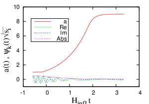
an example of our composite scale factor and a particular dimensionless solution to the evolution equation, where both are plotted versus dimensionless time. This example shows our composite scale factor over a moderate expansion of $\sim 2$ e-folds. The scale factor, $a(t)$ , is continuous, as are $\dot{a}(t)$ and $\ddot{a}(t)$ . The parameters for the first asymptotically flat segment are $a_{1i}=1$ , $a_{2i}=2$ , and $s_{i}=1$ . The free parameters of the end asymptotically flat segment are $a_{2f}=9$ and $a_{1f}=6$ . We choose $b_{i}=b_{f}=0$ . We plot the $k=2$ Fourier mode of $\sqrt{s_{i}}\psi_{k}$ alongside the scale factor to show how this representative evolution solution changes with respect to the scale factor. The real part of $\sqrt{s_{i}}\psi_{k}$ , “Re,” the imaginary part of $\sqrt{s_{i}}\psi_{k}$ , “Im,” and the magnitude of $\sqrt{s_{i}}\psi_{k}$ , “Abs,” are all plotted.

3.1.2.2 Avoidance of Divergent Energy Density

We have checked our method against known mathematical theorems. One such theorem is that in an oscillator with a changing frequency, the quantity $E/\omega$ is conserved if the changes in frequency are made continuously in all derivatives with respect to time; however, if any of the derivatives of the frequency with respect to time are discontinuous, then this introduces changes to the conserved quantity of order $N$ , where the $N$ -th derivative is the first discontinuous derivative [67]. It is also shown by [68] that for adiabatic changes, the changes to the conserved quantity fall off with increasing frequency faster than any power of the frequency. We find in this conserved quantity a close analogy with the average number of particles created per mode for high-energy particles, which are those particles whose wavelengths have not yet exited the Hubble radius before the end of inflation. It is found in Ref. [1], that when the scale factor is changed adiabatically, the amount of particle production falls off with frequency faster than any power of the frequency. The dependence of high-frequency particle production upon the continuity of the scale factor is also noted in [69]. The scale factor must maintain continuity in the zeroth, first, and second derivatives to avoid an ultraviolet divergence in the energy density. This is the reason why we choose matching conditions that are continuous in $a(t)$ , $H(t)$ , and $\dot{H}(t)$ . We could in principle maintain continuity in higher derivatives of our composite scale factor, as well, which would further reduce the amount of high-energy particle production. This further reduction in the high-energy particles would not appreciably improve upon any of our qualitative or quantitative results. The need for $C^{2}$ matching conditions when trying to calculate a finite energy density was previously realized by [61]. In the work of [62, 70] upon the creation of gravitons during inflation, the scale factor is not $C^{2}$ , and both authors adopt a UV-cutoff frequency. The author of [62] recognizes the dependence of high-energy particle production upon the transition from de Sitter space to a radiation dominated universe, and he attributes the entire amount of high-energy particle production to the instantaneous change in the Ricci scalar curvature given by Eq. (2.16) from $12H^{2}$ during inflation to $0$ in a radiation dominated universe. In [3], Parker has shown that massless gravitons satisfying a conformally invariant spin-2 field would not be produced for any $a(t)$ . However, an Einstein graviton that instead satisfied a weak field approximation such as Eq. (4.1), which in vacuum would lead to $\Box\bar{h}_{ab}=0$ , is not conformally invariant. (We use here the definition $\bar{h}_{ab}\equiv h_{ab}-\frac{1}{2}h\eta_{ab}$ , and we work in the Lorentz gauge where $\bar{h}^{ab}{}_{,\beta}=0$ , which means $\bar{h}_{,\beta}=-h_{,\beta}=0$ [17].) This is analogous to a massless, minimally-coupled Klein-Gordon field equation of the form of Eq. (2.87), except for the two polarizations ( $h_{+}$ and $h_{\times}$ ) of gravitational waves [71, 72, 73, 74]. This means that for quanta of this linear field, we would expect the same results for average number of quanta created per mode for each polarization; therefore, $\left|\beta_{k}\right|^{2}_{\rm Einstein\ graviton}=2\left|\beta_{k}\right|^{2}_{\rm scalar}$ .

3.2 Solutions to the Evolution Equation

Consider an inflaton field composed of a spatially homogeneous term plus a first order perturbation,

\phi(\vec{x},t)=\phi^{(0)}(t)+\delta\phi(\vec{x},t).

(3.16)

We investigate, in units of $\hbar=c=1$ , a minimally-coupled scalar field that obeys Eq. (2.90), which we will refer to as the evolution equation:

\partial_{t}^{\ 2}\delta\phi+3H\partial_{t}\delta\phi-a^{-2}(t)\sum_{i=1}^{3}\partial_{i}^{\ 2}\delta\phi+m(\phi^{(0)})^{2}\delta\phi=0.

(3.17)

The mass term is related to the inflationary potential by

m(\phi^{(0)})^{2}=\frac{d^{2}V}{d(\phi^{(0)})^{2}}.

(3.18)

For simplicity, we take $m(\phi^{(0)})^{2}$ as a constant, $m^{2}$ . This is an effective mass, and from now on $m^{2}$ will refer only to this effective mass, which may or may not be the same as the mass of the scalar field, which we will call $m_{\rm scalar}$ . In Eq. (2.78), we show how $m^{2}$ could incorporate a scalar coupling to the background curvature. In what follows, we will assume the minimally coupled case of $\xi=0$ , even though the $m^{2}$ term could include a non-zero coupling term if the curvature were also constant. (In the asymptotically flat segments of our composite scale factor the Ricci scalar curvature is not a constant.) We note that the massless, conformally-coupled case of $m_{\rm scalar}=0$ and $\xi=1/6$ (in a 4-dimensional spacetime) would be conformally-invariant. In the conformally-invariant case the metric tensor and field can be deformed continuously at all points as

	$\displaystyle g_{ab}(x)$	$\displaystyle\rightarrow$	$\displaystyle\tilde{g}_{ab}(x)=\Omega(x)^{2}g_{ab}(x),$		(3.19)
	$\displaystyle\phi(x)$	$\displaystyle\rightarrow$	$\displaystyle\tilde{\phi}(x)=\Omega(x)^{\rm const}\phi(x),$		(3.20)

where $\Omega(x)^{2}$ is a continuous, finite, real, scalar function; in the conformally-invariant case, no particle production occurs [1, 2, 3, 15, 16].

The quantized field $\delta\phi$ can be written in terms of the early time creation and annihilation operators, $A_{\vec{k}}^{\dagger}$ and $A_{\vec{k}}$ , as

\delta\phi=\sum_{\vec{k}}\left(A_{\vec{k}}f_{\vec{k}}+A_{\vec{k}}^{\dagger}f_{\vec{k}}^{*}\right),

(3.21)

where

f_{\vec{k}}=V^{-\frac{1}{2}}e^{i\vec{k}\cdot\vec{x}}\psi_{k}(t(\tau)).

(3.22)

We are imposing periodic boundary conditions upon a cubic coordinate volume, $V=L^{3}$ . In the continuum limit $L$ would go to infinity. The function $\psi_{k}(t)$ satisfies

\partial_{t}^{2}\psi_{k}(t)+3H\partial_{t}\psi_{k}(t)+\frac{k^{2}}{a^{2}(t)}\psi_{k}(t)+m^{2}\psi_{k}(t)=0,

(3.23)

where $k=2\pi n/L$ , with $n$ an integer. Because the creation and annihilation operators in Eq. (3.21) correspond to particles at early times, we require that $\psi_{k}$ satisfies the early-time positive frequency condition

\lim_{\tau\rightarrow-\infty}\psi_{k}(t(\tau))\sim\frac{1}{\sqrt{2a_{1i}{}^{3}\,\omega_{1i}(k)}}e^{-ia_{1i}{}^{3}\,\omega_{1i}(k)\,\tau},

(3.24)

where $\omega_{1i}(k)\equiv\sqrt{(k/a_{1i})^{2}+m^{2}}$ .

At late times, this solution will have the asymptotic form

	$\displaystyle\lim_{\tau^{\prime}\rightarrow\infty}\psi_{k}(t(\tau^{\prime}))$	$\displaystyle\sim$	$\displaystyle\frac{1}{\sqrt{2a_{2f}{}^{3}\,\omega_{2f}(k)}}\bigg[\alpha_{k}e^{-ia_{2f}{}^{3}\,\omega_{2f}(k)\,\tau^{\prime}}$		(3.25)
			$\displaystyle+\beta_{k}e^{ia_{2f}{}^{3}\,\omega_{2f}(k)\,\tau^{\prime}}\bigg],$		(3.25)

where $\omega_{2f}(k)\equiv\sqrt{(k/a_{2f})^{2}+m^{2}}$ .

3.2.1 Joining Conditions

Consider a spacetime composed of three segments of the scale factor, $a(t)$ , in a homogeneous background metric given by Eq. (3.4). For an example, see Figs. 3.1 and 3.3. The first and second segments are joined at the time $t_{1}$ , and the second and third segments are joined at the time $t_{2}$ .

The quantities $\psi_{k}$ and $d\psi_{k}/dt$ are continuous across the joining regions given a continuity of the scale factor of at least $C^{1}$ . Using Eq. (3.47), it is possible to show the conservation of the Wronskian. Multiplying Eq. (3.47) by its conjugate leads to

\frac{d^{2}\psi_{k}(t)^{*}}{d\tau^{2}}\psi_{k}(t)=\frac{d^{2}\psi_{k}(t)}{d\tau^{2}}\psi_{k}(t)^{*}.

(3.26)

Integrating by parts shows

\left[\psi_{k}(t)\frac{d\psi_{k}(t)^{*}}{d\tau}-\psi_{k}(t)^{*}\frac{d\psi_{k}(t)}{d\tau}\right]_{\rm boundary}=0.

(3.27)

Since the boundary conditions are arbitrary, it follows with Eq. (3.7) that the Wronskian,

a(t)^{3}\left[\psi_{k}(t)\frac{d\psi_{k}(t)^{*}}{dt}-\psi_{k}(t)^{*}\frac{d\psi_{k}(t)}{dt}\right],

(3.28)

is a constant. Using Eq. (3.24), we see that this constant is just $i$ ; and using Eq. (3.25), we see that $i\alpha_{k}\alpha_{k}{}^{*}-i\beta_{k}\beta_{k}{}^{*}=i$ , or [1]

\left|\alpha_{k}\right|^{2}-\left|\beta_{k}\right|^{2}=1.

(3.29)

We have two linearly independent solutions to the evolution equation in both the second segment, with solutions $h_{1}(t)$ and $h_{2}(t)$ ; and the third segment, with solutions $g_{1}(t)$ and $g_{2}(t)$ ; for a total of four separate functions. These functions are multiplied by constant coefficients that we must determine. During the second segment, from $t_{1}$ to $t_{2}$ , we have:

	$\displaystyle\psi_{k}(t)=Ah_{1}(t)+Bh_{2}(t),$		(3.30)
	$\displaystyle\psi_{k}^{\prime}(t)=Ah_{1}^{\prime}(t)+Bh_{2}^{\prime}(t).$

For $t>t_{2}$ , we have:

	$\displaystyle\psi_{k}(t)=Cg_{1}(t)+Dg_{2}(t),$		(3.31)
	$\displaystyle\psi_{k}^{\prime}(t)=Cg_{1}^{\prime}(t)+Dg_{2}^{\prime}(t).$

If we require that $\psi_{k}(t)$ and $\psi_{k}^{\prime}(t)$ be continuous at $t_{1}$ and $t_{2}$ . This imposes 4 matching conditions:

	$\displaystyle Ah_{1}(t_{1})+Bh_{2}(t_{1})=\psi_{k}(t_{1}),$		(3.32)
	$\displaystyle Ah_{1}^{\prime}(t_{1})+Bh_{2}^{\prime}(t_{1})=\psi_{k}^{\prime}(t_{1}),$
	$\displaystyle Cg_{1}(t_{2})+Dg_{2}(t_{2})=Ah_{1}(t_{2})+Bh_{2}(t_{2}),$
	$\displaystyle Cg_{1}^{\prime}(t_{2})+Dg_{2}^{\prime}(t_{2})=Ah_{1}^{\prime}(t_{2})+Bh_{2}^{\prime}(t_{2}).$

Given the values of $\psi_{k1}$ and $\psi_{k1}^{\prime}$ , and the matching conditions

$\displaystyle Ah_{1}(t_{1})+Bh_{2}(t_{1})$	$\displaystyle=$	$\displaystyle\psi_{k}(t_{1})=\psi_{k1},$	(3.33)
$\displaystyle Ah_{1}^{\prime}(t_{1})+Bh_{2}^{\prime}(t_{1})$	$\displaystyle=$	$\displaystyle\psi_{k}^{\prime}(t_{1})=\psi_{k1}^{\prime},$
$\displaystyle Cg_{1}(t_{2})+Dg_{2}(t_{2})$	$\displaystyle=$	$\displaystyle Ah_{1}(t_{2})+Bh_{2}(t_{2}),$
$\displaystyle Cg_{1}^{\prime}(t_{2})+Dg_{2}^{\prime}(t_{2})$	$\displaystyle=$	$\displaystyle Ah_{1}^{\prime}(t_{2})+Bh_{2}^{\prime}(t_{2}),$

we wish to calculate the constant coefficients $C$ and $D$ in terms of the functions $h_{1}(t)$ , $h_{2}(t)$ , $g_{1}(t)$ , and $g_{2}(t)$ ; and the values of $\psi_{k1}$ , $\psi_{k1}^{\prime}$ , $t_{1}$ , and $t_{2}$ . (Here a prime denotes derivative with respect to $t$ .) Rearranging the first two matching conditions leads to

	$\displaystyle B=\left[\frac{\psi_{k1}-Ah_{1}}{h_{2}}\right]_{t=t_{1}},$		(3.34)
	$\displaystyle A=\left[\frac{\psi_{k1}^{\prime}-Bh_{2}^{\prime}}{h_{1}^{\prime}}\right]_{t=t_{1}}.$

Combining these two equations leads to

	$\displaystyle A=\left[\frac{\psi_{k1}^{\prime}h_{2}-\psi_{k1}h_{2}^{\prime}}{h_{1}^{\prime}h_{2}-h_{1}h_{2}^{\prime}}\right]_{t=t_{1}},$
	$\displaystyle B=\left[\frac{\psi_{k1}^{\prime}h_{1}-\psi_{k1}h_{1}^{\prime}}{h_{2}^{\prime}h_{1}-h_{2}h_{1}^{\prime}}\right]_{t=t_{1}}.$		(3.35)

At the time $t_{2}$ we have:

$\displaystyle\psi_{k}(t_{2})$	$\displaystyle=$	$\displaystyle Ah_{1}(t_{2})+Bh_{2}(t_{2})$	(3.36)
	$\displaystyle=$	$\displaystyle\bigg\{\left[\frac{\psi_{k1}^{\prime}h_{2}-\psi_{k1}h_{2}^{\prime}}{h_{1}^{\prime}h_{2}-h_{1}h_{2}^{\prime}}\right]_{t=t_{1}}h_{1}(t_{2})$
		$\displaystyle+\left[\frac{\psi_{k1}^{\prime}h_{1}-\psi_{k1}h_{1}^{\prime}}{h_{2}^{\prime}h_{1}-h_{2}h_{1}^{\prime}}\right]_{t=t_{1}}h_{2}(t_{2})\bigg\},$

and

$\displaystyle\psi_{k}^{\prime}(t_{2})$	$\displaystyle=$	$\displaystyle Ah_{1}^{\prime}(t_{2})+Bh_{2}^{\prime}(t_{2})$	(3.37)
	$\displaystyle=$	$\displaystyle\bigg\{\left[\frac{\psi_{k1}^{\prime}h_{2}-\psi_{k1}h_{2}^{\prime}}{h_{1}^{\prime}h_{2}-h_{1}h_{2}^{\prime}}\right]_{t=t_{1}}h_{1}^{\prime}(t_{2})$
		$\displaystyle+\left[\frac{\psi_{k1}^{\prime}h_{1}-\psi_{k1}h_{1}^{\prime}}{h_{2}^{\prime}h_{1}-h_{2}h_{1}^{\prime}}\right]_{t=t_{1}}h_{2}^{\prime}(t_{2})\bigg\}.$

Let us also define $\psi_{k2}\equiv\psi_{k}(t_{2})$ and $\psi_{k2}^{\prime}\equiv\psi_{k}^{\prime}(t_{2})$ . In terms of $\psi_{k2}$ and $\psi_{k2}^{\prime}$ the last two boundary conditions in Eq. (3.33) become

	$\displaystyle C$	$\displaystyle=$	$\displaystyle\left(\frac{\psi_{k2}^{\prime}g_{2}-\psi_{k2}g_{2}^{\prime}}{g_{1}^{\prime}g_{2}-g_{1}g_{2}^{\prime}}\right)_{t=t_{2}},$
	$\displaystyle D$	$\displaystyle=$	$\displaystyle\left(\frac{\psi_{k2}^{\prime}g_{1}-\psi_{k2}g_{1}^{\prime}}{g_{2}^{\prime}g_{1}-g_{2}g_{1}^{\prime}}\right)_{t=t_{2}}.$		(3.38)

Substituting for $\psi_{k2}$ and $\psi_{k2}^{\prime}$ yields

	$\displaystyle C=\left(\frac{[Ah_{1}^{\prime}+Bh_{2}^{\prime}]g_{2}-[Ah_{1}+Bh_{2}]g_{2}^{\prime}}{g_{1}^{\prime}g_{2}-g_{1}g_{2}^{\prime}}\right)_{t=t_{2}},$
	$\displaystyle D=\left(\frac{[Ah_{1}^{\prime}+Bh_{2}^{\prime}]g_{1}-[Ah_{1}+Bh_{2}]g_{1}^{\prime}}{g_{2}^{\prime}g_{1}-g_{2}g_{1}^{\prime}}\right)_{t=t_{2}}.$		(3.39)

Finally, expressing $A$ and $B$ in terms of the given values of $\psi_{k1}$ and $\psi_{k1}^{\prime}$ specified at $t_{1}$ leads to

$\displaystyle C$	$\displaystyle=$	$\displaystyle\frac{1}{\left(g_{1}^{\prime}g_{2}-g_{1}g_{2}^{\prime}\right)_{t=t_{2}}}$	(3.40)
		$\displaystyle\times\bigg\{\left[\frac{\psi_{k1}^{\prime}h_{2}-\psi_{k1}h_{2}^{\prime}}{h_{1}^{\prime}h_{2}-h_{1}h_{2}^{\prime}}\right]_{t=t_{1}}\left(h_{1}^{\prime}g_{2}-h_{1}g_{2}^{\prime}\right)_{t=t_{2}}$
		$\displaystyle+\left[\frac{\psi_{k1}^{\prime}h_{1}-\psi_{k1}h_{1}^{\prime}}{h_{2}^{\prime}h_{1}-h_{2}h_{1}^{\prime}}\right]_{t=t_{1}}\left(h_{2}^{\prime}g_{2}-h_{2}g_{2}^{\prime}\right)_{t=t_{2}}\bigg\},$

and

$\displaystyle D$	$\displaystyle=$	$\displaystyle\frac{1}{\left(g_{2}^{\prime}g_{1}-g_{2}g_{1}^{\prime}\right)_{t=t_{2}}}$	(3.41)
		$\displaystyle\times\bigg\{\left[\frac{\psi_{k1}^{\prime}h_{2}-\psi_{k1}h_{2}^{\prime}}{h_{1}^{\prime}h_{2}-h_{1}h_{2}^{\prime}}\right]_{t=t_{1}}\left(h_{1}^{\prime}g_{1}-h_{1}g_{1}^{\prime}\right)_{t=t_{2}}$
		$\displaystyle+\left[\frac{\psi_{k1}^{\prime}h_{1}-\psi_{k1}h_{1}^{\prime}}{h_{2}^{\prime}h_{1}-h_{2}h_{1}^{\prime}}\right]_{t=t_{1}}\left(h_{2}^{\prime}g_{1}-h_{2}g_{1}^{\prime}\right)_{t=t_{2}}\bigg\},$

which are the combined joining conditions for $\psi_{k}$ and $\psi_{k}^{\prime}$ .

We find $\psi_{k1}$ and $\psi_{k1}^{\prime}$ from the solution to the evolution equation in the initial asymptotically flat segment of the scale factor. In the massless case, this solution is given by Eq. (3.43). The functions $h_{1}(t)$ and $h_{2}(t)$ are to be related to the evolution equation solutions in the inflationary middle segment of the scale factor. Comparing this with Eqs. (3.45) and (3.48) shows $A=E(k)$ and $B=F(k)$ . Similarly, the functions $g_{1}(t)$ and $g_{2}(t)$ are to be related to to the evolution equation solutions in the final asymptotically flat segment of the scale factor, and we will later make the identification $C=N_{1}(k)$ and $D=N_{2}(k)$ , where the coefficients $N_{1}(k)$ and $N_{2}(k)$ are defined through their use in Eq. (3.46).

3.2.2 Exact Massless Solutions

We will first consider the case, $m=0$ . Rewriting the evolution equation, Eq. (3.23), in terms of $\tau$ instead of $t$ leads to

\frac{d^{2}\psi_{k}}{d\tau^{2}}=-k^{2}a^{4}\psi_{k}.

(3.42)

For the first segment of our composite scale factor, the solution of (3.42) having positive frequency form (3.24) at early times is the hypergeometric function [4, 16, 65, 66]

	$\displaystyle\psi_{k}(t(\tau))$	$\displaystyle=$	$\displaystyle\frac{1}{\sqrt{2a_{1i}{}^{2}k}}e^{-ika_{1i}{}^{2}\tau}F(-ika_{1i}{}^{2}s_{i}+ika_{2i}{}^{2}s_{i},$		(3.43)
			$\displaystyle-ika_{1i}{}^{2}s_{i}-ika_{2i}{}^{2}s_{i};1-2ika_{1i}{}^{2}s_{i};-e^{\frac{\tau}{s_{i}}}),$		(3.43)

where $F(a,b;c;d)$ is the hypergeometric function as defined in [21, see 15.1.1]:

F(a,b;c;z)=\frac{\Gamma(c)}{\Gamma(a)\Gamma(b)}\sum_{n=0}^{\infty}\frac{\Gamma(a+n)\Gamma(b+n)}{\Gamma(c+n)}\,\frac{z^{n}}{n!}.

(3.44)

For the exponentially expanding segment of the scale factor in the massless case ( $V^{\prime\prime}=0$ in Eq. (2.99) above)

\psi_{k}(t)=a(t)^{-\frac{3}{2}}\left[E(k)H_{\frac{3}{2}}^{(1)}\left(\frac{k}{a(t)H_{\rm infl}}\right)+F(k)H_{\frac{3}{2}}^{(2)}\left(\frac{k}{a(t)H_{\rm infl}}\right)\right],

(3.45)

where $H^{(1)}$ and $H^{(2)}$ are the Hankel functions of the first and second kind. The variables $t$ and $\tau$ are related by Eq. (3.7). The coefficients $E(k)$ and $F(k)$ are determined by the matching conditions of the first joining point at $t=t_{1}$ . We note that the finite period of exponential inflation lacks the full symmetries of a de Sitter universe. In the pure de Sitter case, as shown in [20], the $k=0$ mode has to be chosen in a special way to avoid infrared divergences. For our $a(t)$ , infrared divergences do not arise (see Sec. 3.2.2).

For the final segment of our composite scale factor, the solution of the evolution equation (3.42) is a linear combination of hypergeometric functions [4, 16, 65, 66]:

$\displaystyle\psi_{k}(t(\tau^{\prime}))$	$\displaystyle=$	$\displaystyle N_{1}(k)e^{-ika_{1f}{}^{2}\tau^{\prime}}F(-ika_{1f}{}^{2}s_{f}+ika_{2f}{}^{2}s_{f},$	(3.46)
		$\displaystyle-ika_{1f}{}^{2}s_{f}-ika_{2f}{}^{2}s_{f};1-2ika_{1f}{}^{2}s_{f};-e^{\frac{\tau^{\prime}}{s_{f}}})$
		$\displaystyle+N_{2}(k)e^{ika_{1f}{}^{2}\tau^{\prime}}F(ika_{1f}{}^{2}s_{f}+ika_{2f}{}^{2}s_{f},$
		$\displaystyle ika_{1f}{}^{2}s-ika_{2f}{}^{2}s_{f};1+2ika_{1f}{}^{2}s_{f};-e^{\frac{\tau^{\prime}}{s_{f}}}),$

where the coefficients $N_{1}(k)$ and $N_{2}(k)$ are determined by the matching conditions of the second joining point at $t=t_{2}$ . An example of the evolution for a particular mode is plotted for a specific choice of parameters using our composite scale factor in Figs. 3.3 and 3.4.

Fig. 3.4 shows

a dimensionless solution to the massless evolution equation, where the $k=2$ Fourier mode is plotted versus dimensionless time for the same composite scale factor used in Fig. 3.1. The real part of $\sqrt{s_{i}}\psi_{k}$ , the imaginary part of $\sqrt{s_{i}}\psi_{k}$ , and the magnitude of $\sqrt{s_{i}}\psi_{k}$ are all plotted.

With joining conditions for the segments of the scale factor, the derived solution to the evolution equation can be matched up with the known solution for the exponential expansion of an inflationary segment by matching $\delta\phi_{k}(t)$ and its time derivative across the boundary conditions. See Figure 3.5

for the evolution of modes in the middle of a long inflationary period for the massless case. The time $t$ is taken to be zero when $k=a(t)H$ (when the plotted mode exits the Hubble radius) and depends on the mode number $k$ . Multiplied by $k^{3}/H_{\rm inflation}^{2}$ and plotted against this mode-dependent time, all of the different fluctuation modes align along the same curve in this graph. This shows, in the massless case, the scale-invariance of the spectrum for those modes that exit the Hubble radius during a period of constant $H(t)$ .

3.2.3 Approximations to Massive Solution

In the case of a massive scalar field, the evolution equation, Eq. (3.23), can be written in terms of $\tau$ as

\frac{d^{2}\psi_{k}}{d\tau^{2}}=-(k^{2}a^{4}+m^{2}a^{6})\psi_{k}.

(3.47)

For the middle, inflationary segment of our scale factor, our solution given by Eq. (2.99) is

\psi_{k}(t)=a(t)^{-\frac{3}{2}}\left[E(k)H_{\sqrt{\frac{9}{4}-m_{H}^{\ 2}}}^{(1)}\left(\frac{k}{a(t)H_{\rm infl}}\right)+F(k)H_{\sqrt{\frac{9}{4}-m_{H}^{\ 2}}}^{(2)}\left(\frac{k}{a(t)H_{\rm infl}}\right)\right],

(3.48)

where we define $m_{H}$ in terms of the effective mass by

m_{H}\equiv\frac{m}{H_{\rm infl}}.

(3.49)

We know the solution to the evolution equation for the region of the scale factor given by Eq. (3.5) exactly, but we do not have an analytic solution for an asymptotically flat segment of our scale factor except for the trivial case of a constant scale factor. We instead use one of two different approximations that we find reduce to the same numerical solutions in their mutual realms of applicability: the effective-k approach and the dominant-term approach.

3.2.2.1 Effective-k Approach

In the first of these approximations, the effective-k approach, we choose our initial and final asymptotically flat segments of the scale factor such that $a_{1i}\simeq a_{2i}$ and $a_{1f}\simeq a_{2f}$ . The middle segment of our scale factor, under these conditions, is thus where almost all of the change in the scale factor occurs, and we make use of our exact solution in this region. In the beginning and final asymptotically flat segments we make the transformation $k\rightarrow k_{\rm eff}$ , where $k_{\rm eff}$ is an effective $k$ defined in the initial region as

k_{i\,\rm eff}\equiv\sqrt{k^{2}+m^{2}a_{1i}^{\ \ 2}},

(3.50)

and in the final region by

k_{f\,\rm eff}\equiv\sqrt{k^{2}+m^{2}a_{2f}^{\ \ 2}}.

(3.51)

In the limit that $a_{2}=a_{1}$ in a given segment, the approximation becomes exact and reduces to the known Minkowski flat space solution of

\psi_{k}(t(\tau))=\frac{1}{\sqrt{2a^{3}\omega}}\left[\alpha_{k}e^{-ia^{3}\omega\tau}+\beta_{k}e^{ia^{3}\omega\tau}\right],

(3.52)

where $\omega$ is given by

\omega\equiv\sqrt{\frac{k^{2}}{a^{2}}+m^{2}}.

(3.53)

The closer the ratio $a_{2}/a_{1}$ comes to unity in an asymptotically flat segment of the scale factor, the more trustworthy the effective-k approach becomes. If the two parameters are precisely equal, however, then the scale factor becomes a constant in time and derivatives of the scale factor are equal to zero. In such a case where $a_{2}=a_{1}$ , we cannot join to the inflationary middle segment continuously in any derivatives of the scale factor. When $a_{1f}\simeq a_{2f}$ in the end segment of our composite scale factor, we observe ultraviolet particle production due to the rapid breaking, or deceleration, of the scale factor’s expansion. This is true regardless of effective mass, because this “extended” region of particle production occurs where the mass is negligible and $(k/a(t))^{2}\gg m^{2}$ .

3.2.2.2 Dominant Term Approach

The Effective- $k$ Approach works very well— especially for the case where the final asymptotically flat scale factor is parameterized such that $a_{1f}\simeq a_{2f}$ . The Effective- $k$ Approach need not be as accurate when $a_{1f}\ll a_{2f}$ , and for this situation we introduce an alternate massive approximation, that of the Dominant Term Approach. In this case we introduce a new asymptotically flat scale factor that yields an exact solution in the limit that $k\rightarrow 0$ . For a fixed mass, this approximation becomes exceedingly close to the exact solution whenever $|m|\gg k/a(t)$ . In the Dominant Term Approach, when $k/a\gg|m|$ , we use the asymptotically flat scale factor given above along with the massless solution; and when $|m|\gg k/a(t)$ , we use a new asymptotically flat scale factor and its associated zeroth Fourier mode solution. These two solutions can be matched up for the case of modes in the intermediary- $q_{2}$ region, where we would use the massless solution for the initial asymptotically flat scale factor and the massive solution for the final asymptotically flat scale factor. The Dominant Term Approach is suspect at the interface between the small- and intermediary- $q_{2}$ behaviors and at the interface between the intermediary- and large- $q_{2}$ behaviors, where the justification for neglecting either the $m$ -term or the $k/a$ -term is weakest. Depending upon which term is neglected, however, this method provides tight upper and lower limits on the average particle production per mode even at these interfaces. When an abrupt transition from the exponential inflation of the middle scale factor segment to the asymptotically flat final scale factor segment is taken to make a fair comparison, the Dominant Term Approach is in excellent agreement with the Effective- $k$ Approach— even at the interfaces of $q_{2}\simeq 1$ and $q_{2}\simeq\exp(-N_{e})$ . When the final transition between the second and third scale factor segments is not taken to be abrupt, the upper- and lower-limits place the results of the Dominant Term Approach very close to the Effective- $k$ Approach— even at the interfaces— and they differ only in their descriptions of the large- $q_{2}$ behavior. This is because the Effective- $k$ Approach requires an abrupt end to inflation and is not a contradiction between the two approaches, but rather is a result of the previously mentioned fact that an abrupt transition at the end of inflation produces a high-energy region of residual particle production.

Inflaton Field of Fixed Mass and Zeroth Fourier Mode

In units of $\hbar=c=1$ , the perturbations to the inflaton field satisfy the evolution equation for mode- $k$

\ddot{\delta\phi_{k}}+3H(t)\dot{\delta\phi_{k}}+\frac{k^{2}}{a(t)^{2}}\delta\phi_{k}+m^{2}\delta\phi_{k}=0;

(3.54)

where a dot represents a derivative with respect to the proper time; where $a(t)$ is the scale factor; where $H(t)\equiv\dot{a(t)}/a(t)$ is the Hubble constant, which may vary with time; and where $m$ is taken to be a constant effective inflaton mass, which is equal to the square root of the second derivative of the inflationary potential with respect to the homogeneous, background part of the inflaton field. With a change of variables from the proper time, $t$ , to a new time variable that satisfies the relationship $d\tau\equiv a(t)^{-3}dt$ ; and examining the zeroth Fourier mode, where $k=0$ , which can in fact can be taken to be approximately correct whenever $k/a(t)\ll m$ , the evolution equation becomes

\frac{d^{2}\delta\phi_{0}}{d\tau^{2}}=-m^{2}a(\tau)^{6}\delta\phi_{0}.

(3.55)

Using an analysis patterned after that which Epstein used to model the scattering of radio waves off the ionosphere [63] and that which Eckart used to model potential energy in one-dimensional scattering in quantum mechanics [64], we define a scale factor that is asymptotically flat in both the past- and future-time infinities as

a(\tau)=\bigg\{a_{1}^{\ 6}+e^{\tau/s}[(a_{2}^{\ 6}-a_{1}^{\ 6})(e^{\tau/s}+1)+b](e^{\tau/s}+1)^{-2}\bigg\}^{\frac{1}{6}}.

(3.56)

The form of this scale factor is modeled after the scale factor first introduced by Parker [4, 16, 65, 66] which has four adjustable parameters $a_{1}$ , $a_{2}$ , $s$ , and $b$ that allow one to approximate a wide range of possible scale factors $a(\tau)$ . The field equation, Eq. (3.55), with this scale factor, $a(\tau)$ , has exact solutions in terms of hypergeometric functions [63, 64]. With this scale factor, Eq. (3.55) becomes

\frac{d^{2}\delta\phi_{0}}{d\tau^{2}}=-m^{2}\left\{a_{1}^{\ 6}+e^{\tau/s}[(a_{2}^{\ 6}-a_{1}^{\ 6})(e^{\tau/s}+1)+b](e^{\tau/s}+1)^{-2}\right\}\delta\phi_{0}.

(3.57)

A change of variables to $u\equiv e^{\tau/s}$ leads to

\frac{d^{2}\delta\phi_{0}}{d(s\ln u)^{2}}=-m^{2}\left\{a_{1}^{\ 6}+u[(a_{2}^{\ 6}-a_{1}^{\ 6})(u+1)+b](u+1)^{-2}\right\}\delta\phi_{0}.

(3.58)

With the chain rule, we use

$\displaystyle\frac{d^{2}\delta\phi_{0}}{d(s\ln u)^{2}}$	$\displaystyle=$	$\displaystyle\frac{1}{s^{2}}\left(\frac{d\ln u}{du}\right)^{-1}\frac{d}{du}\left[\left(\frac{d\ln u}{du}\right)^{-1}\frac{d}{du}\delta\phi_{0}\right]$	(3.59)
	$\displaystyle=$	$\displaystyle\frac{u}{s^{2}}\frac{d}{du}\left[u\frac{d}{du}\delta\phi_{0}\right]$
	$\displaystyle=$	$\displaystyle\frac{u^{2}}{s^{2}}\frac{d^{2}}{du^{2}}\delta\phi_{0}+\frac{u}{s^{2}}\frac{d}{du}\delta\phi_{0}$

to write, with a prime denoting a derivative with respect to the variable $u$ ,

\delta\phi_{0}^{\prime\prime}+\frac{\delta\phi_{0}^{\prime}}{u}+\frac{s^{2}m^{2}}{u^{2}}\left\{a_{1}^{\ 6}+u[(a_{2}^{\ 6}-a_{1}^{\ 6})(u+1)+b](u+1)^{-2}\right\}\delta\phi_{0}=0.

(3.60)

Without having yet made any assumption as to the reality of $\tau/s$ , the variable $u$ may range from $-\infty$ to $+\infty$ on the complex plane. Portions of this evolution equation can be seen to become infinite at $u=0$ and $u=-1$ . For the case of $u=0$ , where the evolution equation becomes

\delta\phi_{0}^{\prime\prime}+\frac{\delta\phi_{0}^{\prime}}{u}+\frac{s^{2}m^{2}}{u^{2}}a_{1}^{\ 6}\delta\phi_{0}=0,

(3.61)

we use the chain rule to change variables to $v=\ln u$ , where $\partial_{u}=u^{-1}\partial_{v}$ , to get

e^{-v}\partial_{v}\left(e^{-v}\partial_{v}\delta\phi_{0}\right)+e^{-2v}\partial_{v}\delta\phi_{0}+e^{-2v}s^{2}m^{2}a_{1}^{\ 6}\delta\phi_{0}=0,

(3.62)

which simplifies to

\partial_{v}{}^{2}\delta\phi_{0}=-s^{2}m^{2}a_{1}^{\ 6}\delta\phi_{0},

(3.63)

the solution of which is,

\delta\phi_{0}=e^{\pm isma_{1}{}^{3}v}=u^{\pm isma_{1}{}^{3}}.

(3.64)

For the case of $u=-1$ , where the evolution equation becomes

\delta\phi_{0}^{\prime\prime}-\delta\phi_{0}^{\prime}+s^{2}m^{2}\left\{a_{1}{}^{6}-b(u+1)^{-2}\right\}\delta\phi_{0}=0,

(3.65)

we test the analog of the solution found in Eq. (3.64) to look for a solution of the form

\delta\phi_{0}=(u+1)^{x},

(3.66)

and insert this into the evolution equation for the case of $u=-1$ to find

x(x-1)(u+1)^{x-2}-x(u+1)^{x-1}+s^{2}m^{2}a_{1}{}^{6}(u+1)^{x}-s^{2}m^{2}b(u+1)^{x-2}=0.

(3.67)

Because $(u+1)=0$ , the factors with the lowest exponential power of $(u+1)^{x-2}$ dominate this equation, and at the point of $u=-1$ the evolution equation obeys

x(x-1)(u+1)^{x-2}=s^{2}m^{2}b(u+1)^{x-2},

(3.68)

x(x-1)=s^{2}m^{2}b,

(3.69)

with solutions

x_{\pm}=\frac{1\pm\sqrt{1+4s^{2}m^{2}b}}{2},

(3.70)

so at $u=-1$

\delta\phi_{0}=(u+1)^{x_{\pm}}.

(3.71)

A second order differential equation has at most two distinct solutions; therefore, our test has found all the solutions for the case of $u=-1$ . To write the $u=0$ case in an equivalent form, we define

p_{1}\equiv isma_{1}{}^{3},

(3.72)

such that for the $u=0$ case

\delta\phi_{0}=u^{\pm p_{1}},

(3.73)

and define for later use

p_{2}\equiv isma_{2}{}^{3}.

(3.74)

To find the general solution of $\delta\phi_{0}(u)$ , we write

\delta\phi_{0}=(1+u)^{x_{-}}u^{-p_{1}}f[u],

(3.75)

where the function $f[u]$ is defined by this equation. We insert this expression for $\delta\phi_{0}$ back into Eq. (3.60) to get

	$\displaystyle 0$	$\displaystyle=$	$\displaystyle\left((1+u)^{x_{-}}u^{-p_{1}}f[u]\right)^{\prime\prime}+\frac{\left((1+u)^{x_{-}}u^{-p_{1}}f[u]\right)^{\prime}}{u}$		(3.76)
			$\displaystyle+\frac{s^{2}m^{2}}{u^{2}}\left\{a_{1}^{\ 6}+u[(a_{2}^{\ 6}-a_{1}^{\ 6})(u+1)+b](u+1)^{-2}\right\}(1+u)^{x_{-}}u^{-p_{1}}f[u],$		(3.76)

which, with $s^{2}m^{2}a_{1,2}{}^{6}=-p_{1,2}{}^{2}$ and $s^{2}m^{2}b=x_{-}x_{+}=x_{-}{}^{2}-x_{-}$ , becomes

$\displaystyle 0$	$\displaystyle=$	$\displaystyle x_{-}(x_{-}-1)(1+u)^{x_{-}-2}u^{-p_{1}}f[u]-p_{1}x_{-}(1+u)^{x_{-}-1}u^{-p_{1}-1}f[u]+x_{-}(1+u)^{x_{-}-1}u^{-p_{1}}f^{\prime}[u]$	(3.77)
		$\displaystyle-p_{1}x_{-}(1+u)^{x_{-}-1}u^{-p_{1}-1}f[u]+p_{1}(p_{1}+1)(1+u)^{x_{-}}u^{-p_{1}-2}f[u]-p_{1}(1+u)^{x_{-}}u^{-p_{1}-1}f^{\prime}[u]$
		$\displaystyle+x_{-}(1+u)^{x_{-}-1}u^{-p_{1}}f^{\prime}[u]-p_{1}(1+u)^{x_{-}}u^{-p_{1}-1}f^{\prime}[u]+(1+u)^{x_{-}}u^{-p_{1}}f^{\prime\prime}[u]$
		$\displaystyle+\frac{x_{-}(1+u)^{x_{-}-1}u^{-p_{1}}f[u]-p_{1}(1+u)^{x_{-}}u^{-p_{1}-1}f[u]+(1+u)^{x_{-}}u^{-p_{1}}f^{\prime}[u]}{u}$
		$\displaystyle+\frac{1}{u^{2}}\left\{-p_{1}{}^{2}+u[(-p_{2}{}^{2}+p_{1}{}^{2})(u+1)+x_{-}x_{+}](u+1)^{-2}\right\}(1+u)^{x_{-}}u^{-p_{1}}f[u],$

multiplying by $(1+u)^{-x_{-}+1}u^{p_{1}+1}$ produces

$\displaystyle 0$	$\displaystyle=$	$\displaystyle x_{-}(x_{-}-1)(1+u)^{-1}uf[u]-p_{1}x_{-}f[u]+x_{-}uf^{\prime}[u]$	(3.78)
		$\displaystyle-p_{1}x_{-}f[u]+p_{1}(p_{1}+1)(1+u)u^{-1}f[u]-p_{1}(1+u)f^{\prime}[u]$
		$\displaystyle+x_{-}uf^{\prime}[u]-p_{1}(1+u)f^{\prime}[u]+(1+u)uf^{\prime\prime}[u]$
		$\displaystyle+\frac{x_{-}uf[u]-p_{1}(1+u)uf[u]+(1+u)uf^{\prime}[u]}{u}$
		$\displaystyle+\frac{u+1}{u}\left\{-p_{1}{}^{2}+u[(-p_{2}{}^{2}+p_{1}{}^{2})(u+1)+x_{-}x_{+}](u+1)^{-2}\right\}f[u],$

which can be simplified to

$\displaystyle 0$	$\displaystyle=$	$\displaystyle u(u+1)f^{\prime\prime}+[2x_{-}u-2p_{1}(1+u)+(1+u)]f^{\prime}$	(3.79)
		$\displaystyle+\bigg[x_{-}(x_{-}-1)(1+u)^{-1}u-2p_{1}x_{-}+x_{-}+[p_{1}(p_{1}+1)-p_{1}](1+u)u^{-1}$
		$\displaystyle+\frac{u+1}{u}\left\{-p_{1}{}^{2}+u[(-p_{2}{}^{2}+p_{1}{}^{2})(u+1)+x_{-}x_{+}](u+1)^{-2}\right\}\bigg]f,$

which can be further simplified to

$\displaystyle 0$	$\displaystyle=$	$\displaystyle u(u+1)f^{\prime\prime}+[2x_{-}u-2p_{1}(1+u)+(1+u)]f^{\prime}$	(3.80)
		$\displaystyle+\bigg[([x_{-}{}^{2}-x_{-}]u+x_{-}x_{+})(u+1)^{-1}+(p_{1}{}^{2}-p_{1}{}^{2})u^{-1}$
		$\displaystyle+(-2p_{1}x_{-}+p_{1}{}^{2}-p_{2}{}^{2}+p_{1}{}^{2}-p_{1}{}^{2}+x_{-})\bigg]f,$

then to

	$\displaystyle 0$	$\displaystyle=$	$\displaystyle u(u+1)f^{\prime\prime}+[2x_{-}u-2p_{1}(1+u)+(1+u)]f^{\prime}$		(3.81)
			$\displaystyle+\left(-2p_{1}x_{-}+p_{1}{}^{2}-p_{2}{}^{2}+x_{-}{}^{2}\right)f,$		(3.81)

and finally to

	$\displaystyle 0$	$\displaystyle=$	$\displaystyle u(u+1)f^{\prime\prime}+[(2x_{-}-2p_{1}+1)u+(1-2p_{1})]f^{\prime}$		(3.82)
			$\displaystyle+(x_{-}-p_{1}+p_{2})(x_{-}-p_{1}-p_{2})f.$		(3.82)

This is a hypergeometric equation and can be solved in terms of the hypergeometric function $f=F(x_{-}-p_{1}+p_{2},x_{-}-p_{1}-p_{2};1-2p_{1};-u)$ , using the notation of [21].

Joining Scale Factors Continuously to Second Derivative

To achieve a finite energy density we must maintain the continuity of the composite scale factor to $C^{2}$ at the matching points of the individual scale factor segments. Sec. 3.3.1 discusses further the need for $C^{2}$ joining conditions. See Figure 3.6

for an example of the asymptotically flat scale factor described in the previous section joined to a region of inflation where the scale factor grows exponentially with respect to proper time. This graph shows how an asymptotically flat region could be joined onto the beginning or end of an exponential region.

To join these different scale factors continuously to the second derivative, we note that an exponentially growing scale factor, of the form $a(t)=a_{0}\exp(Ht)$ , has a time-independent Hubble constant. To find a point in the asymptotically flat scale factor described above where $\dot{H}=0$ , we must find a local extremum of $H(t)$ . When $b=0$ , there is a unique maximum value of $H(t)$ . In a simpler scale factor of the form $a(t)\propto t^{n}$ , which describes a radiation- or matter-dominated universe, no such point would exist. Using the relationship $d\tau\equiv a(t)^{-3}dt$ , the Hubble constant is $H(t)\equiv a(t)^{-1}(da/dt)=a(\tau)^{-4}(da/d\tau)$ , and its time-derivative is $\dot{H}(t)=a(\tau)^{-3}\partial_{\tau}[a(\tau)^{-4}\partial_{\tau}a(\tau)]=a(\tau)^{-7}\partial_{\tau}{}^{2}a(\tau)-4a(\tau)^{-8}[\partial_{\tau}a(\tau)]^{2}$ . This is zero when $(d^{2}a(\tau)/d\tau^{2})=4a(\tau)^{-1}(da/d\tau)^{2}$ ; in other words, when

	$\displaystyle\left[\frac{\left\{\frac{1}{3}-\frac{1}{6}(1+e^{-\tau/s})e^{\tau/s}\right\}(1+e^{-\tau/s})^{-3}(a_{2}^{\ 6}-a_{1}^{\ 6})e^{-2\tau/s}}{s^{2}\left[a_{1}^{\ 6}+(1+e^{-\tau/s})^{-1}(a_{2}^{\ 6}-a_{1}^{\ 6})\right]^{\frac{5}{6}}}\right]$	(3.83)
	$\displaystyle+\left[\frac{-\frac{5}{36}(1+e^{-\tau/s})^{-4}(a_{2}^{\ 6}-a_{1}^{\ 6})^{2}e^{-2\tau/s}}{s^{2}\left[a_{1}^{\ 6}+(1+e^{-\tau/s})^{-1}(a_{2}^{\ 6}-a_{1}^{\ 6})\right]^{\frac{11}{6}}}\right]$
$\displaystyle=$	$\displaystyle 4\left[a_{1}^{\ 6}+(1+e^{-\tau/s})^{-1}(a_{2}^{\ 6}-a_{1}^{\ 6})\right]^{-\frac{1}{6}}\left[\frac{\frac{1}{6}(1+e^{-\tau/s})^{-2}(a_{2}^{\ 6}-a_{1}^{\ 6})e^{-\tau/s}}{s\left[a_{1}^{\ 6}+(1+e^{-\tau/s})^{-1}(a_{2}^{\ 6}-a_{1}^{\ 6})\right]^{\frac{5}{6}}}\right]^{2},$

where the parameter $b$ in Eq. (3.60) has been taken to be zero so that there might be a unique maximum value of the Hubble constant. To simplify this, we multiply both sides of the equation by $12s^{2}a(\tau)^{\frac{11}{6}}(a_{2}{}^{6}-a_{1}{}^{6})^{-1}(1+e^{-\tau/s})^{4}e^{3\tau/s}$ to get

	$\displaystyle\left(\left\{4e^{\tau/s}-2(1+e^{-\tau/s})e^{2\tau/s}\right\}\left[a_{1}^{\ 6}(1+e^{-\tau/s})+(a_{2}^{\ 6}-a_{1}^{\ 6})\right]\right)$
	$\displaystyle+\left(-\frac{5}{3}(a_{2}^{\ 6}-a_{1}^{\ 6})e^{\tau/s}\right)=\left(\frac{4}{3}(a_{2}^{\ 6}-a_{1}^{\ 6})e^{\tau/s}\right),$		(3.84)

which can be expressed as

2a_{2}{}^{6}e^{2\tau/s}+(a_{2}{}^{6}-a_{1}{}^{6})e^{\tau/s}-2a_{1}{}^{6}=0.

(3.85)

This is a quadratic equation with two roots for $e^{\tau/s}$ . The ratio $\tau/s$ is now taken to be real, which means $e^{\tau/s}$ is non-negative; this leaves only the positive root solution of

e^{\tau/s}=\frac{a_{1}{}^{6}-a_{2}{}^{6}+\sqrt{a_{1}{}^{12}+14a_{1}{}^{6}a_{2}{}^{6}+a_{2}{}^{12}}}{4a_{2}{}^{6}}.

(3.86)

Once that is found, the $C^{2}$ matching conditions for $\tau$ , $a(\tau$ ), and $H$ are

$\displaystyle\tau$	$\displaystyle=$	$\displaystyle s\ln\left[\frac{a1_{1}^{\ 6}-a_{2}^{\ 6}+\sqrt{a_{1}{}^{12}+14a_{1}{}^{6}a_{2}{}^{6}+a_{2}{}^{12}}}{4a_{2}^{\ 6}}\right],$	(3.87)
$\displaystyle a(\tau)$	$\displaystyle=$	$\displaystyle\left(\frac{a_{2}^{\ 6}(5a_{1}^{\ 6}-a_{2}^{\ 6}+\sqrt{a_{1}{}^{12}+14a_{1}{}^{6}a_{2}{}^{6}+a_{2}{}^{12}})}{a_{1}^{\ 6}+3a_{2}^{\ 6}+\sqrt{a_{1}{}^{12}+14a_{1}{}^{6}a_{2}{}^{6}+a_{2}{}^{12}}}\right)^{\frac{1}{6}},$	(3.88)
$\displaystyle H$	$\displaystyle=$	$\displaystyle\left(\frac{\sqrt{2}(-a_{1}^{\ 6}+a_{2}^{\ 6})}{3a_{2}^{\ 6}(5a_{1}^{\ 6}-a_{1}^{\ 6}+\sqrt{a_{1}{}^{12}+14a_{1}{}^{6}a_{2}{}^{6}+a_{2}{}^{12}})^{2}\ s}\right)$	(3.89)
		$\displaystyle\times(a_{1}^{\ 6}-a_{2}^{\ 6}+\sqrt{a_{1}{}^{12}+14a_{1}{}^{6}a_{2}{}^{6}+a_{2}{}^{12}})$
		$\displaystyle\times\sqrt{-a_{1}^{\ 6}-a_{2}^{\ 6}+\sqrt{a_{1}{}^{12}+14a_{1}{}^{6}a_{2}{}^{6}+a_{2}{}^{12}}}.$

3.3 Particle Creation

At late times, our solution to the evolution equation will have the asymptotic form given by Eq. (3.25). The early- and late-time vacua are related through a Bugoliubov Transformation [1] (alternately Romanized in the literature from the Cyrillic as Bugolubov or Bugolyubov or Bogoliubov), where the early-time creation and annihilation operators ( $A_{\vec{k}}^{\dagger}$ and $A_{\vec{k}}$ ) are related to the late-time creation and annihilation operators ( $a_{\vec{k}}^{\dagger}$ and $a_{\vec{k}}$ ) through

a_{\vec{k}}=\alpha_{k}A_{\vec{k}}+\beta_{k}^{*}A_{\vec{k}}^{\dagger},

(3.90)

where $\alpha_{k}$ and $\beta_{k}$ are the Bugoliubov coefficients given by Eq. (3.25) and satisfying Eq. (3.29). Because our scale factor is asymptotically Minkowskian, the meaning of particles at early and late times has no ambiguity. At late times, the number operator is

\langle N_{\vec{k}}\rangle_{t\rightarrow\infty}=\langle 0|a_{\vec{k}}^{\dagger}a_{\vec{k}}|0\rangle=\left|\beta_{k}\right|^{2},

(3.91)

where $\left|0\right>$ is the state annihilated by the early-time annihilation operators $A_{\vec{k}}$ . For the rest of this chapter, the notation $\left|\delta\phi_{k}\right|^{2}$ is defined as $\langle 0\left|\delta\phi_{k}\delta\phi_{k}\right|0\rangle=|f_{\vec{k}}|^{2}$ . In the continuum limit, this reduces to $(2\pi)^{-3}|\psi_{k}|^{2}$ . Thus, $\left|\beta_{k}\right|^{2}$ is the average number of particles in mode- ${\vec{k}}$ created by the expansion of the scale factor from a state that initially has no particles [1, 3].

3.3.1 Dependence on Mode, Expansion, and Mass

In the absence of units, the magnitudes of $k$ , $a$ , $H$ , and $m$ have no inherent significance. The ratio of the Hubble radius, $H^{-1}$ , to wavelength, $a/k$ , however, does have significance. This combination of $k/aH$ is what we call $q_{2}$ when we take the particular values of $a=a_{2f}$ and $H=H_{\rm infl}$ . The other relevant dimensionless ratios are $m_{H}\equiv m/H_{\rm infl}$ and $N_{e}$ . Transformations that simultaneously leave the values of $k/(a(t)H(t))$ and $m_{H}$ intact do not change the arguments of any of the evolution solutions used in our composite scale factor. See Eq. (3.48) for the inflationary middle segment of our composite scale factor. For an asymptotically flat scale factor of either the form described by Eq. (3.6) or the form described by Eq. (3.56), no matter how we scale $a=a(\tau/s,a_{1},a_{2})$ , the ratio $a_{2}/a_{1}$ remains a constant; furthermore, when keeping the particular value of $\tau/s$ fixed, $H\propto 1/(sa_{1}^{\ 3})\propto 1/(sa_{2}^{\ 3})$ . For example, if we multiply $k$ by a constant and multiply $a(t)$ by that same constant, we don’t change the wavelength of our mode. If we don’t alter $H$ , this rescaling won’t change $\left|\beta_{q_{2}}\right|^{2}$ . When $b=0$ , we see that this transformation is

$\displaystyle k\rightarrow$	$\displaystyle k*x$
$\displaystyle a_{1}\rightarrow$	$\displaystyle a_{1}*x$
$\displaystyle a_{2}\rightarrow$	$\displaystyle a_{2}*x$
$\displaystyle s\rightarrow$	$\displaystyle s*x^{-3}.$	(3.92)

For a second example, rescaling $k$ , $H_{\rm infl}$ , and $m$ by the same factor is equivalent to

$\displaystyle k\rightarrow$	$\displaystyle k*y$
$\displaystyle s\rightarrow$	$\displaystyle s*y^{-1}$
$\displaystyle m\rightarrow$	$\displaystyle m*y.$	(3.93)

This second example won’t change the average number of particles created per mode, either. We note that in the massless case the coefficient $1/\sqrt{2a_{1i}{}^{2}k}$ from Eq. (3.43) may change in invariant transformations, but $\left|\beta_{q_{2}}\right|^{2}$ does not change because Eqs. (3.94) and (3.95) contain factors that compensate for the change in $N_{1}$ . The same is true in the massive case under the transformation $k/a(t)\rightarrow\sqrt{(k/a(t))^{2}+m^{2}}$ .

In the massless case we find the following:

For our choice of the final asymptotically flat segment given by Eq. (3.6), where we use Eq. (3.46) to define our functions $g_{1}(t)$ and $g_{2}(t)$ in terms of the relationship $\psi_{k}(t)=N_{1}g_{1}(t(\tau))+N_{2}g_{2}(t(\tau))$ , we find the coefficients $\alpha_{k}$ and $\beta_{k}$ of Eq. (3.25) from the large argument asymptotic forms [4, 16, 65, 66, 21]. With $b_{f}=0$ , $c_{1}\equiv iks_{f}a_{1f}^{\ \ 2}$ , and $c_{2}\equiv iks_{f}a_{2f}^{\ \ 2}$ , we have

\alpha_{k}=\sqrt{2ka_{2f}^{\ \ 2}}\left[\frac{C\ \Gamma(1-2c_{1})\Gamma(-2c_{2})}{\Gamma(1-c_{1}-c_{2})\Gamma(-c_{1}-c_{2})}+\frac{D\ \Gamma(1+2c_{1})\Gamma(-2c_{2})}{\Gamma(1+c_{1}-c_{2})\Gamma(c_{1}-c_{2})}\right],

(3.94)

and

\beta_{k}=\sqrt{2ka_{2f}^{\ \ 2}}\left[\frac{C\ \Gamma(1-2c_{1})\Gamma(2c_{2})}{\Gamma(1-c_{1}+c_{2})\Gamma(-c_{1}+c_{2})}+\frac{D\ \Gamma(1+2c_{1})\Gamma(2c_{2})}{\Gamma(1+c_{1}+c_{2})\Gamma(c_{1}+c_{2})}\right].

(3.95)

Recall that $C$ and $D$ and the functions $g_{1}(t)$ and $g_{2}(t)$ were defined in Sec. 3.2.1. A useful check of our method is the test of whether Eq. (3.29) is validated, which we find to be true in all our numerical calculations.

The variable $\left|\beta_{k}\right|^{2}$ is the average number of particles created in the mode k, as measured at late times, from the expansion of the scale factor through $N_{e}$ number of e-folds, starting from a universe that is initially in a vacuum state that is asymptotically Minkowskian. We use the dimensionless variable

q_{2}\equiv\frac{k}{a_{2f}H_{\rm infl}},

(3.96)

where k is the wave number, $a_{2f}$ is the asymptotically flat late-time scale factor, and $H_{\rm infl}$ is the constant value of $\left({\dot{a}(t)}/{a(t)}\right)$ — where the dot represents a derivative with respect to proper time— during the exponential expansion of the middle segment. We express our results using $q_{2}$ instead of the wave number, $k$ , because we find that $|\beta_{q_{2}}|^{2}$ is an invariant quantity (see Fig. 3.7), whereas $|\beta_{k}|^{2}$ depends on the arbitrary value of the scale factor. By $|\beta_{q_{2}}|^{2}$ , we refer to the average number of particles created in the mode given by $k=q_{2}H_{\rm infl}a_{2f}$ . See the end of Sec. 3.4.3 for a discussion of invariant transformations.

We define three regions of $q_{2}$ . Values of $q_{2}\lesssim\exp(-N_{e})$ are in the small- $q_{2}$ region. Values of $\exp(-N_{e})\lesssim q_{2}\lesssim 1$ are in the intermediary- $q_{2}$ region. Values of $1\lesssim q_{2}$ are in the large- $q_{2}$ region.

Fig. 3.7 shows the

average late time particle number per mode ( $|\beta_{q_{2}}|^{2}$ ) versus $q_{2}=k/(a_{2f}H_{\rm infl})$ for 60 e-folds of inflation. Two cases are plotted for the massless case based on the behavior at the matching conditions: the scale factor continuous in 0th, 1st, and 2nd derivatives ( $C^{2}$ ); and the scale factor continuous in 0th and 1st derivatives ( $C^{1}$ ). Note that in the $C^{1}$ case, $\left|\beta_{q_{2}}\right|^{2}$ transitions from a $q_{2}^{\ -2}$ dependence at the end of the intermediary- $q_{2}$ region all the way to a $q_{2}^{\ -6}$ dependence, temporarily parallel to the $C^{2}$ large- $q_{2}$ regime, before settling down into its ultraviolet $q_{2}^{\ -4}$ behavior. For the wiggles near the transition from the small- $q_{2}$ region to the intermediary- $q_{2}$ region at $q_{2}=e^{-N_{e}}$ , compare with the graph of the dispersion spectrum in Fig. 3.11.

When $a(t)$ is $C^{1}$ or $C^{2}$ , i.e. when $H_{\rm infl}$ is continuous, we find numerically that the particle production per mode in the small- $q_{2}$ region, ( $q_{2}\lesssim e^{-N_{e}}$ ), is

\beta_{q_{2}}=\sinh[N_{e}].

(3.97)

We also find this to be the case, analytically, by taking the limit $k\rightarrow 0$ . This analytical limit can be seen as follows. Eq. (3.42), in the $k\rightarrow 0$ limit tells us that $d\psi_{k}(\tau)/d\tau$ is constant. From Eq. (3.24), we see that at early times $\psi_{k}(\tau)=1/\sqrt{2ka_{1i}{}^{2}}$ and $d\psi_{k}(\tau)/d\tau=-i\sqrt{ka_{1i}{}^{2}/2}\rightarrow 0$ in the $k\rightarrow 0$ limit. Because $d\psi_{k}(\tau)/d\tau$ is both constant and zero, so must $\psi_{k}(\tau)$ be constant. Matching $\psi_{k}(\tau)$ and $d\psi_{k}(\tau)/d\tau$ with the late-time conditions— which do not make any assumptions about the changing scale factor before the late-time asymptotically flat region of spacetime is reached— leads to two boundary conditions:

1/\sqrt{2ka_{1i}{}^{2}}=(\alpha_{k}+\beta_{k})/\sqrt{2ka_{2f}{}^{2}},

(3.98)

-i\sqrt{ka_{1i}{}^{2}/2}=(-i\alpha_{k}+i\beta_{k})\left(\sqrt{ka_{2f}{}^{2}/2}\right).

(3.99)

This leads to

\alpha_{k}+\beta_{k}=e^{N_{e}},

(3.100)

\alpha_{k}-\beta_{k}=e^{-N_{e}}.

(3.101)

The solution to this is

\alpha_{k}=\cosh N_{e},

(3.102)

\beta_{k}=\sinh N_{e}.

(3.103)

In the limit of $k\rightarrow 0$ , both coefficients happen to be real, and we can see that Eq. (3.29) is naturally satisfied. Although this result was derived in the $k\rightarrow 0$ limit, it is valid in the massless case whenever $k/(a_{1i}H_{\rm infl})\ll 1$ . This small- $q_{2}$ limit holds for arbitrary expansions, besides those described by our parameterized composite scale factor, provided they initiate from a Minkowski vacuum state. We find that the requirement for an alternative to the Bunch-Davies state for the $k=0$ mode in de Sitter space would be a consequence of taking $N_{e}\rightarrow\infty$ in this analytical limit.

For at least a moderate number of e-folds, this simplifies to

|\beta_{q_{2}}|^{2}\simeq\frac{1}{4}e^{2N_{e}}.

(3.104)

The dependence in the intermediary- $q_{2}$ region ( $e^{-N_{e}}\lesssim q_{2}\lesssim 1$ ) for the $C^{2}$ or $C^{1}$ massless case is

|\beta_{q_{2}}|^{2}\simeq\frac{1}{4}q_{2}^{\ -2}.

(3.105)

When $N_{e}$ is finite, with our composite scale factor there are no infrared divergences. For infinite inflation, where $N_{e}\rightarrow\infty$ , we find the infrared divergences of a de Sitter universe. This problem is resolved for a true de Sitter universe in [20]. Our composite scale factor is different from a purely de Sitter universe in that our initial conditions are specified by our initial asymptotically flat region of the scale factor.

Discontinuities in the derivatives of the scale factor at the matching points introduce additional particle production for modes in the large- $q_{2}$ (or $q_{2}\gtrsim 1$ ) region. For the $C^{1}$ case, where the scale factor and $H=\dot{a}(t)/a(t)$ are both continuous, the large- $q_{2}$ region goes like

|\beta_{q_{2}}|^{2}=n_{4}q_{2}^{-4}.

(3.106)

For the $C^{2}$ case, where the scale factor and $H=\dot{a}(t)/a(t)$ and $\dot{H}(t)$ are all continuous, the large- $q_{2}$ region goes like

|\beta_{q_{2}}|^{2}=n_{6}q_{2}^{-6}.

(3.107)

Here $n_{4}$ and $n_{6}$ are constant coefficients, with $n_{4}\simeq n_{6}\simeq\mathcal{O}(1/4)$ for a gradual end to inflation. For a sufficiently abrupt end to inflation, $n_{4}$ and $n_{6}$ can be made to be arbitrarily large. See Sec. 3.7.

In the $C^{0}$ case, $H(t)$ is not continuous, and we find quite a different behavior. The evolution equation, Eq. (3.23), may be written [3]

\frac{d^{2}\psi_{k}(t)}{dt^{2}}+\left[\frac{k^{2}}{a(t)^{2}}+m^{2}-\frac{3}{4}\left(\frac{\dot{a}(t)}{a(t)}\right)^{2}-\frac{3}{2}\frac{\ddot{a}(t)}{a(t)}\right]\psi_{k}(t)=0.

(3.108)

At the discontinuity in $\dot{a}(t)$ , if we express the jump as a step function, then the form of $\ddot{a}(t)$ picks up a delta-function contribution. Thus, there is a finite jump in $d\psi_{k}(t)/dt$ across the discontinuity. The Wronskian is still conserved. In the $C^{0}$ case, $\left|\beta_{q_{2}}\right|^{2}$ is proportional to $q_{2}^{\ -2}$ in the small- and large- $q_{2}$ regions, and it is proportional to $q_{2}^{\ -4}$ in the intermediary- $q_{2}$ region. A $C^{0}$ scenario would suffer from both infrared and ultraviolet divergences, hence we will not consider it further.

For a non-composite scale factor composed of one asymptotically flat scale factor defined by Eq. (3.6), at large values of $q_{2}$ the value of $|\beta_{q_{2}}|^{2}$ falls off faster than any power of $q_{2}$ , and in terms of $k$ we have: [4, 16, 65, 66]

|\beta_{k}|^{2}=\frac{\sin^{2}\left(\frac{1}{2}[1-\sqrt{1+4k^{2}s^{2}b}]\right)+\sinh^{2}[\pi ks(a_{1}^{\ 2}-a_{2}^{\ 2})]}{\sinh^{2}[\pi ks(a_{1}^{\ 2}+a_{2}^{\ 2})]-\sinh^{2}[\pi ks(a_{1}^{\ 2}-a_{2}^{\ 2})]}.

(3.109)

In the limit that $k\rightarrow 0$ for the case of the scale factor of Eq. (3.6), which is asymptotically flat at early and late times and has no exponential segment, we find that $\lim_{k\rightarrow 0}\left|\beta_{k}\right|^{2}=\sinh^{2}[N_{e}]$ , where in this case $N_{e}$ is $\ln\left(a_{2}/a_{1}\right)$ . This is the same small- $q_{2}$ limit for the average number of particles created per mode as we found above in Eq. (3.97). The analog of the intermediary- $q_{2}$ region extends over a range of $\ln q_{2}$ equal to $2N_{e}$ , as opposed to $N_{e}$ for the particle production associated with our composite scale factor. Thus, a graph of the average number of particles created per mode for a single asymptotically flat scale factor would look similar to Fig 3.7, except the region analogous to the intermediary- $q_{2}$ region would be twice as long and would have half the slope relative to a scale factor dominated by an exponential expansion.

In the massive case we find the following:

In Fig. 3.8,

the dependence of particle production ( $\left|\beta_{q_{2}}\right|^{2}$ ) on mass is shown for an expansion of 60 e-folds. The beginning and end segments are defined by $a_{2i}=a_{1i}(1+10^{-26})$ , $a_{2f}=a_{1i}e^{60}$ , and $a_{1f}=0.9999a_{2f}$ . The massless case can be compared with the plot in Fig. 3.7 which is continuous up to the second derivative of the scale factor to see that the two graphs are the same for $q_{2}\lesssim 1$ . In this graph, however, there is an “extended” region of $\left|\beta_{q_{2}}\right|^{2}\propto q_{2}^{-2}$ shortly after $q_{2}\simeq 1$ that lasts until $q_{2}\simeq 10^{4}$ before the ultraviolet behavior of $\left|\beta_{q_{2}}\right|^{2}\propto q_{2}^{-6}$ is seen. The term “extended” is defined in Sec. 3.7. This is due to particle creation caused by the rapid transition from the inflationary region to the asymptotically flat scale factor. The two approximations, the effective-k approach and the dominant-term approach, give the same results with this particular parameterization of inflation. Both of the massive cases shown here produce more red-shifted particles of low momentum than the massless case. The case of $m_{H}^{2}=1/10$ produces many more low momentum particles than the case of $m_{H}^{2}=1$ . See also Figs. 3.9 and 3.13.

In Fig. 3.9,

the dependence of particle production ( $\left|\beta_{q_{2}}\right|^{2}$ ) on mass is shown for an expansion of 60 e-folds. This graph is different from Fig. 3.8 in that the transition from exponential expansion to the final asymptotic segment of the scale factor is more gradual, happening over about an e-fold. Thus, we use the dominant-term approximation. The effective-k approach, in spite of the gradual transition to an asymptotically flat scale factor, overlaps with the dominant-term approach in this graph except very close to $q_{2}=1$ . For values of $q_{2}\lesssim 1$ , this graph is identical to that of Fig. 3.8.

3.3.2 Limit of Negligible Mass with Respect to H

In Fig. 3.10,

particle production as a function of $q_{2}$ is plotted for 60 e-folds for both the massless case and the case of $m=10^{-10}H_{\rm infl}$ , labeled as $m<<H$ . This graph was made using the dominant-term approximation. The effective-k approach would overlap on this graph except very near to $q_{2}=m_{H}=10^{-10}$ . It is always the case that $(k/a(t))^{2}\gg m^{2}$ for $q_{2}>m_{H}$ and in this region the plot of $m_{H}=10^{-10}$ overlaps with the massless case. For $q_{2}<m_{H}\exp(-N_{e})$ , relative to the mass we can take $k=0$ , and in this region of $q_{2}$ in the tiny mass case of $m_{H}\ll 1$ , the value of $\left|\beta_{q_{2}}\right|^{2}$ approaches the constant $(1/4)q_{2}^{\ 3N_{e}}$ . In the region of $m_{H}\exp(-N_{e})<q_{2}<m_{H}$ , we have $(k/a(t))^{2}\gg m^{2}$ in the initial asymptotically flat region and $(k/a(t))^{2}\ll m^{2}$ in the final asymptotically flat region. Between $q_{2}\simeq m_{H}\exp(-N_{e})$ and $q_{2}\simeq\exp(-N_{e})$ , we see $\left|\beta_{q_{2}}\right|^{2}\propto q_{2}^{\ -1}$ ; and between $q_{2}\simeq\exp(-N_{e})$ and $q_{2}\simeq m_{H}$ , we see $\left|\beta_{q_{2}}\right|^{2}\propto q_{2}^{\ -3}$ . In light of these characteristics, a comparison of Eqs. (3.115) and (3.116) can be made with consideration to where $(k/a(t))^{2}\gg m^{2}$ and to where $(k/a(t))^{2}\ll m^{2}$ . Such an analysis shows that in the tiny mass limit of $m_{H}\ll 1$ , the dispersion spectrum reduces to the massless dispersion spectrum. The tiny mass limit bridges the transition from the massless case to the case of small, non-negligible $m_{H}$ such as $m_{H}=0.01$ , and the dispersion spectra as a function of $q_{2}$ for all cases changes continuously when going from massless to tiny mass to small mass. This is a successful check on our method.

3.4 Dispersion Spectrum

The dispersion spectrum is [16, 75]

\left<\ \right|\delta\phi^{2}\left|\ \right>=\frac{1}{2(a_{2f}L)^{3}}\sum_{k}\left[\frac{1+2|\beta_{k}|^{2}}{\sqrt{(k/a_{2f})^{2}+m^{2}}}\right].

(3.110)

We will first consider the massless case where $m=0$ . See below in Sec. 3.4.3 for the massive case. We subtract off the late-time Minkowski vacuum contribution, which is that part of the unrenormalized dispersion which would be present in a Minkowski vacuum without any particles ( $\left|\beta_{k}\right|^{2}=0$ for all $k$ ), to get the dispersion

	$\displaystyle\left<\ \right\|\delta\phi^{2}\left\|\ \right>$		$\displaystyle=\frac{1}{2(a_{2f}L)^{3}}\sum_{k}\frac{2\|\beta_{k}\|^{2}}{\sqrt{(k/a_{2f})^{2}}}$		(3.111)
			$\displaystyle=\frac{1}{a_{2f}^{\ \ 2}L^{3}}\sum_{k}\frac{\|\beta_{k}\|^{2}}{k},$		(3.111)

which in the continuum limit becomes

\left<\ \right|\delta\phi^{2}\left|\ \right>=\frac{1}{a_{2f}^{\ \ 2}(2\pi)^{3}}\int_{0}^{\infty}\frac{|\beta_{k}|^{2}}{k}d^{3}k.

(3.112)

Spherical symmetry, where $d^{3}k=4\pi k^{2}dk$ , gives us

\left<\ \right|\delta\phi^{2}\left|\ \right>=\frac{1}{2\pi^{2}a_{2f}^{\ \ 2}}\int_{0}^{\infty}k|\beta_{k}|^{2}dk.

(3.113)

With $k=q_{2}a_{2f}H_{\rm infl}$ and $dk=dq_{2}a_{2f}H_{\rm infl}$ , we have

	$\displaystyle\left<\ \right\|\delta\phi^{2}\left\|\ \right>$		$\displaystyle=\frac{a_{2f}^{\ \ 2}H_{\rm infl}^{2}}{2\pi^{2}a_{2f}^{\ \ 2}}\int_{0}^{\infty}q_{2}\|\beta_{q_{2}}\|^{2}dq_{2}$		(3.114)
			$\displaystyle=\frac{H_{\rm infl}^{2}}{2\pi^{2}}\int_{0}^{\infty}q_{2}\|\beta_{q_{2}}\|^{2}dq_{2}.$		(3.114)

In the massless case, the dispersion spectrum amplitude is thus

Z\equiv\frac{q_{2}|\beta_{q_{2}}|^{2}H_{\rm infl}^{2}}{2\pi^{2}}.

(3.115)

We plot $Z/H_{\rm infl}^{2}$ in Fig. 3.11. We see that in both the case where $a(t)$ , $\dot{a}(t)$ , and $\ddot{a}(t)$ are all continuous; and the case where $a(t)$ and $\dot{a}(t)$ are continuous; $\left<\ \right|\delta\phi^{2}\left|\ \right>$ is finite without the need for any renormalization beyond subtracting off the Minkowski vacuum terms. When none of the derivatives of the scale factor is continuous, then the dispersion spectrum does not converge.

Fig. 3.11 shows the dispersion spectrum $Z/H_{\rm infl}^{2}$ given by Eq. (3.115) for our composite scale factor continuous in $a(t)$ , $\dot{a}(t)$ , and $\ddot{a}(t)$ over an expansion of 60 e-folds. The y-axis, $Z/H_{\rm infl}^{2}$ , is shown multiplied by a factor of $e^{-N_{e}}$ ; and the x-axis, $q_{2}$ , is shown multiplied by a factor of $e^{N_{e}}$ . When using this scaling, the region plotted in this graph would look identical for an expansion of 10 e-folds, and it would look identical for an expansion of 80 e-folds. In the case of $a_{2i}=a_{1i}+w$ , where $w\equiv 10^{-26}a_{1i}$ , we see marked peaks in the dispersion spectrum. When we change the parameters in the initial asymptotically flat region to $a_{2i}=10a_{1i}$ , these peaks are damped as shown. The ending conditions of the final asymptotically flat segment do not affect these peaks.

A calculation of the dispersion spectrum in the massive case leads to an equation analogous to Eq. (3.115):

Z\equiv\frac{q_{2}|\beta_{q_{2}}|^{2}H_{\rm infl}^{2}}{2\pi^{2}\sqrt{1+\frac{m_{H}^{\ 2}}{q_{2}^{\ 2}}}}.

(3.116)

3.4.1 Sensitivity to Initial Conditions

We take for our initial conditions a quantum state to be asymptotic at early times to that of a Minkowski vacuum spacetime for all modes. This is a consequence of our asymptotically flat scale factor and our assumption that no particles are initially present. It is more common in the literature to take instead the Bunch-Davies state for quantum fluctuations, that is to assume a de Sitter spacetime. As pointed out by [62], this leads to an infrared divergence of the two-point function, where the two-point function is another name for our dispersion spectrum, and the cause of this divergence is correctly diagnosed as being due to the choice of initial conditions in [70]. Both of the authors of [62, 70] handle these infrared divergences with a cutoff frequency that omits modes that are currently outside the Hubble radius of our observable universe.

The use of de Sitter initial conditions is equivalent to supposing an inflationary period that extends over an infinite number of e-folds, or $N_{e}\rightarrow\infty$ . If we assume a finite $N_{e}$ , and if we assume that in the future our universe will be approximately matter-dominated for all times, which means neglecting any dark energy or cosmological constant, then eventually every mode that exited the Hubble radius during inflation would eventually re-enter the Hubble radius of our universe after inflation if it has not already done so.

Both Figs. 3.11 and 3.12 show additional peaks after the primary peak, where the primary peak roughly indicates the interface between small- $q_{2}$ and intermediary- $q_{2}$ behavior. These minor peaks are caused by phase differences between modes with similar wavelengths as they exit the Hubble radius near the beginning of inflation. The modes that exit the Hubble radius with a large amplitude— either a positive real amplitude, a negative real amplitude, a positive imaginary amplitude, or a negative imaginary amplitude— quickly have this large amplitude translated into a near constant value outside of the Hubble radius. Those modes that exit the Hubble radius with relatively small amplitudes are frozen into evolutions of relatively small magnitudes outside of the Hubble radius; these relatively low-amplitude modes have a relatively high change in amplitude with respect to time, but this initial excess in the derivative of the amplitude with respect to time is rapidly redshifted away during inflation. With an abrupt transition from an asymptotically Minkowski vacuum to an exponential inflation of the scale factor, by which we mean that $a(t_{1})\simeq a_{1i}$ , where $a(t_{1})$ is the scale factor at the transition from the initial asymptotically flat segment to the exponentially growing segment of inflation, and where $a_{1i}$ is the scale factor at early times, we see that the minor peaks are more pronounced. With a more gradual transition from the initial asymptotically flat segment of the scale factor to inflation (when $a(t_{1})\simeq 1.2a_{1i}$ ), these minor peaks are damped out. If these modes were observable in our universe, that is if they have already re-entered our Hubble radius, their measurement might tell us something about initial conditions before the beginning of inflation: whether there had been a phase transition from the very early universe to inflation, how rapidly the very early universe had been expanding (or contracting) relative to the expansion of inflation, and what the dominant contribution to the evolution of our universe might have been before the start of inflation. Because measuring the contribution of these minor wiggles to the scale dependence of large-scale structure would be experimentally challenging (if not impossible), this is in some sense speculation, but that does not change the fact that the two dispersion spectra shown in Fig. 3.11 are different, and this difference— if observed— would tell us about our pre-inflationary universe.

3.4.2 Sensitivity to Sub-Planck Length Physics

Consider a quantum fluctuation of the particular mode that, at the beginning of inflation, has a wavelength equal to the Planck length. By the time this wavelength has been stretched to the point that the mode is exiting the Hubble radius, it will have a wavelength the size of the Hubble radius. For this to happen, the scale factor must increase by a factor of $H_{\rm infl}^{-1}/\ell_{\rm Planck}$ .

With $\hbar=c=1$ , the Planck length is $\ell_{\rm Planck}=\sqrt{G}=8\times 10^{-20}\ {\rm(GeV)}^{-1}$ . Using the value of $H_{\rm infl}=7\times 10^{13}$ GeV given in Eq.(2.149), we find $H_{\rm infl}^{-1}/\ell_{\rm Planck}\simeq 2\times 10^{5}$ , which corresponds to a mode exiting the Hubble radius $\ln(10^{7})\simeq 12$ e-folds after the start of inflation. All higher frequency modes, that is for $q_{2}\gtrsim e^{-N_{e}+12}$ , will have originated from trans-Planckian modes during inflation. With $N_{e}=60$ e-folds of inflation, if we use the estimate of the number of e-folds before the end of inflation in which the observable modes of the CMB are exiting the Hubble radius given by Eq. (2.143) (50 e-folds) or by Eq. (3.144) (53 e-folds), then it might be possible to observe the difference in amplitudes between those modes that were initially super-Planckian quantum fluctuations and those that were initially sub-Planckian quantum fluctuations before the start of inflation. With either a smaller value of the Hubble constant during inflation or with a larger number of total e-folds of inflation, the re-entry of the first trans-Planckian modes back into our Hubble radius after inflation could be postponed to epochs of our universe much later than recombination.

3.4.3 Model in Terms of Expansion and Mass

Fig. 3.12 shows

a comparison of the dispersion spectrum ( $Z/H_{\rm infl}^{2}$ ) given by Eq. (3.116) and normalized to 1 for our composite scale factor continuous in $a(t)$ , $\dot{a}(t)$ , and $\ddot{a}(t)$ over an expansion of 60 e-folds for various masses. The values of $Z/H_{\rm infl}^{2}$ were divided by the maximum value of the primary peak for each located at $q_{2}\simeq\exp(-N_{e})$ . To normalize these peaks, $Z/H_{\rm infl}^{2}$ was divided by the following factors: $1.3\times 10^{24}$ for the massless case, $2.3\times 10^{22}$ for $m_{H}^{\ 2}=0.1$ , and $2.2\times 10^{4}$ for $m_{H}^{\ 2}=1$ .

The dispersion spectrum is plotted for three different cases of $m_{H}$ in Fig. 3.12. The effective-k approach is useful for this approximation. This approach demands that in the initial asymptotically flat segment of the scale factor, $a(t)$ must always be approximately equal to $a_{1i}$ . Because $a(t_{1})\simeq a_{1}$ if either $a_{2}\simeq a_{1}$ or $a_{2}\gg a_{1}$ , however, this approach can be used with a wide range of initial conditions. Specifically, when $a_{2}\gg a_{1}$ in Eq. (3.6), we have $a(t_{1})\simeq(7/3)^{(1/4)}$ . Although we are not at the moment considering the case of $a_{2}\gg a_{1}$ in Eq. (3.56), for comparison we note that it would lead to $a(t_{1})\simeq 3^{(1/6)}$ . In both cases $a(t_{1})\simeq 1.2a_{1}$ . We have found that, even in the massive case, the observed humps are dependent only upon the initial conditions. In the region shown in this figure, the graph would not be significantly altered by using $C^{1}$ joining conditions instead of our $C^{2}$ matching conditions. The effective-k approximation plotted on this graph would overlap with the exact solution, if an exact solution were available. The shapes of the curves are fixed above a moderate number of e-folds. We define the variable $J$ such that the maximum value of $Z/H_{\rm infl}^{2}$ for the major peak, which is the peak located nearest to $q_{2}=e^{-N_{e}}$ , is $J\ e^{(P-1)N_{e}}$ in the massless case and is $J\ e^{(P-2)N_{e}}$ in the massive case. Then, the normalization factor scales like $e^{(P-1)N_{e}}$ in the massless case, as can be seen from Eq. (3.115); and the normalization factor scales like $e^{(P-2)N_{e}}$ in the massive case, as can be seen from Eq. (3.116), where we define the exponent $P$ in the following way:

\left|\beta_{q_{2}}\right|^{2}\simeq\frac{1}{4}q_{2}^{\ -P}

(3.117)

in the region of intermediary- $q_{2}$ ( $e^{-N_{e}}\lesssim q_{2}\lesssim 1$ ), and

\left|\beta_{q_{2}}\right|^{2}\simeq\frac{1}{4}e^{PN_{e}}

(3.118)

in the small- $q_{2}$ region ( $q_{2}\lesssim e^{-N_{e}}$ ). The exponent $P$ is well described by a $q_{2}$ -independent value in the case of $m=0$ and in the case of $0.01\lesssim m_{H}^{\ 2}\lesssim 9/4$ .

In the massless case, $P=2$ , so the height of the major peak in the graph of the massless case in Fig. 3.12 grows with an increasing number of e-folds as $e^{N_{e}}$ , while the widths of the peaks narrow with an increasing number of e-folds as $e^{-N_{e}}$ . The area under an individual peak in the massless graph therefore does not change appreciably when changing the number of e-folds of expansion, provided there are at least a few e-folds of inflation. For the massive cases, we see that $P=2.93358$ when $m_{H}^{\ 2}=0.1$ , and that $P=2.23607$ when $m_{H}=1$ .

Fig. 3.13 shows

the dependence of the variable $P$ , as defined in Eq. (3.117), upon $m_{H}=m/H_{\rm infl}$ . The calculated data points shown lie on the curve $P=\sqrt{9-4m_{H}^{\ 2}}$ . Outside of the region plotted, however, $P$ does not have a constant, $q_{2}$ -independent value. For $m_{H}>1.5$ , the argument, $\sqrt{(9/4)-m_{H}^{\ 2}}$ , of the Hankel functions becomes imaginary, and $\left|\beta_{q_{2}}\right|^{2}$ oscillates with changing $q_{2}$ . For an example of a non-zero mass much smaller than $H_{\rm infl}$ , see Fig. 3.10.

We wish now to approximate the dependence of the configuration space dispersion $\left<\ \right|\delta\phi^{2}\left|\ \right>/H_{\rm infl}^{2}$ with regard to the number of e-folds. In our approximation we neglect the minor peaks; we assume that the major peak is located exactly at $q_{2}=e^{-N_{e}}$ , that $Z/H^{2}$ increases linearly with $q_{2}$ up to the major peak, and that $Z/H^{2}$ decreases as $(q_{2}e^{N_{e}})^{2-P}$ in the massive case— or as $(q_{2}e^{N_{e}})^{1-P}$ in the massless case— until the onset of large- $q_{2}$ behavior at $q_{2}=1$ , which effectively serves as a cut-off point. The maximum of the major peak is given by $\textrm{height}=J\ e^{(P-2)N_{e}}$ , in the massive case; and $\textrm{height}=J\ e^{(P-1)N_{e}}$ , in the massless case. We find $J\simeq 0.01$ for all three cases. In this simple approximation, the configuration space dispersion is given by TABLES 3.1 and 3.2.

Table 3.1: Approximation

	$\left<\ \right\|\delta\phi^{2}\left\|\ \right>/H_{\rm infl}^{2}$
$0.01\lesssim m_{H}\lesssim 1.49$	$\frac{1}{2}J\ e^{(P-3)N_{e}}+\int_{e^{-N_{e}}}^{1}dq_{2}\ J\ q_{2}^{2-P}$
$m_{H}=0$	$\frac{1}{2}J+\int_{e^{-N_{e}}}^{1}dq_{2}\ J\ q_{2}^{1-P}$

Table 3.2: Configuration Space Dispersion

	$\left<\ \right\|\delta\phi^{2}\left\|\ \right>/H_{\rm infl}^{2}$
$0.01\lesssim m_{H}\lesssim 1.49$	$\left(\frac{1}{3-P}+\frac{1-P}{6-2P}e^{(P-3)N_{e}}\right)J$
$m_{H}=0$	$\left(\frac{1}{2}+N_{e}\right)J$

The small mass limit of $P\rightarrow 3$ and the massless case of $P=2$ , both reduce to the same limit of

\left|\delta\phi\right|\simeq\frac{H_{\rm infl}}{10}\sqrt{N_{e}+\frac{1}{2}}.

(3.119)

For further discussion of the small mass limit reducing to the massless dispersion spectrum, see Fig. 3.10.

3.5 Scalar Spectral Index and Scale Invariance

We define a given mode of $\delta\phi_{k}$ to be crossing the Hubble radius when $k/(a(t)H(t))=1$ . We define a mode of $k$ to be inside the Hubble radius when $k>a(t)H(t)$ , and we define a mode of $k$ to be outside the Hubble radius when $k<a(t)H(t)$ . Modes in the intermediary- $q_{2}$ range exit during inflation to eventually re-enter the Hubble radius at some time after inflation has ended, provided any cosmological constant or dark energy can be taken to be negligible. Using our composite scale factor, we note that after a few e-folds of inflation, the quantum perturbations that are exiting the Hubble radius are found numerically to satisfy

\displaystyle\left|\psi_{k}\right|^{2}=\frac{H_{\rm infl}^{2}}{k^{3}D(m_{H})},

(3.120)

where $\left|\psi_{k}\right|^{2}$ is the time-dependent part of $\left|\delta\phi_{k}\right|^{2}$ , as given by Eqs. (3.21) and (3.22). The variable $D(m_{H})\simeq(1+\frac{1}{5}m_{H}^{\ 2})^{2}$ is a constant of order 1 that we have evaluated numerically to be

$\displaystyle D(m_{H}=0)$	$\displaystyle=$	$\displaystyle 1.00,$
$\displaystyle D(m_{H}=\sqrt{0.1})$	$\displaystyle=$	$\displaystyle 1.04,$
$\displaystyle D(m_{H}=1)$	$\displaystyle=$	$\displaystyle 1.45.$	(3.121)

Thus, our spectrum of $\left|\delta\phi_{k}\right|^{2}$ , if evaluated at the time of exiting the Hubble radius, is scale-invariant, regardless of effective mass. By Eqs. (2.124) and (2.125) we have

\mathcal{P}_{\mathcal{R}}\propto k^{3}\left|\delta\phi_{k}\right|^{2}.

(3.122)

The scalar spectral index given by Eq.(2.127) is

n_{s}=1+\frac{d\ln\mathcal{P}_{\mathcal{R}}}{d\ln k}.

(3.123)

We see that when taken at the time of crossing the Hubble radius, the spectrum, which is proportional to $k^{3}\left|\delta\phi_{k}\right|^{2}$ , has no k-dependence because we have shown the spectrum is proportional to $k^{0}\,H_{\rm infl}^{2}/D(m_{H})$ . Evaluating the scalar spectral index at the time of exiting the Hubble radius thus leads to $n_{s}=1$ , which can be used as the definition of a scale-invariant spectrum.

The modes that exit the Hubble radius at the very beginning of inflation, however, along with those that exit the Hubble radius before reaching the middle segment of our composite scale factor where $a(t)$ begins to grow exponentially with respect to $t$ , are not described by Eq. (3.120). These modes in the small- $q_{2}$ region are not scale-invariant; therefore, well after the end of inflation, long-wavelength modes that are not scale-invariant would eventually re-enter the Hubble radius of a matter-dominated universe. If the total number of e-folds of inflation is sufficiently small, it would be possible to observe a transition from the scale-invariance to a scale-dependence of large-scale structure. See Figs. 3.7, 3.8, and 3.9. Because the small- $q_{2}$ modes of large enough wavelength exit the Hubble radius before evolving away from the early-time conditions specified by Eq. (3.24), we would expect a massless inflaton to generate a spectral index of $n_{s}=3$ in the small- $q_{2}$ region, and we would expect a massive inflaton to generate a spectral index of $n_{s}=4$ in the small- $q_{2}$ region. If scale-invariance continued indefinitely for large wavelength modes, the dispersion would be infrared divergent, so this eventual end to scale-invariance is not an artifact of our initial conditions. The modes responsible for the galaxy-size structure of today left the Hubble radius approximately 45 e-folds before the end of inflation [9, p. 285], so if $N_{e}$ were not too much larger than this, we would expect it to be possible to measure the end of scale-invariance in our observable universe.

In Fig. 3.14 we plot six scenarios depicting the behavior of $\left|\psi_{k}\right|^{2}$ after exiting the Hubble radius. The first two cases, A and B, are for $m_{H}=0$ . In both of these cases, an expansion of 20 total e-folds is plotted. In case A, there is a gradual end to inflation spanning one e-fold; and in case B, there is an abrupt end to inflation. Because the mode has exited the Hubble radius, neither of these end conditions changes $\left|\delta\phi_{k}\right|^{2}$ , and the two lines overlap. Here, and in general for the massless case, $\left|\delta\phi_{k}\right|^{2}$ reaches a constant value a few e-folds after exiting the Hubble radius, and this constant value is close to the value at the time of exit. In the massless case, we find a scale-invariant spectrum even when the spectrum is defined in terms of the value of $\left|\delta\phi_{k}\right|^{2}$ at the end of inflation. This can be found by noting that at the time a particular mode is crossing the Hubble radius, the value of $\left|\psi_{k}\right|^{2}$ given by Eq. (3.45) is approaching a constant value as the argument $k/[a(t)H_{\rm infl}]$ becomes much less than 1.

For cases labeled C, D, E, and F; we use $m_{H}=\sqrt{0.1}$ . In the massive cases, $\left|\psi_{k}\right|^{2}$ never reaches a constant value, although it changes much more slowly after exiting the Hubble radius. Cases C and D are the massive analogs of cases A and B, respectively. In case E, we end inflation gradually over the length of one e-fold, starting just as our specific mode crosses the Hubble radius. In case F, we end inflation abruptly just as our specific mode crosses the Hubble radius.

From [21], {Eq. 9.1.9}, we see that in the small argument limit of the Hankel functions

\left|H_{v}^{(1)}(z)\right|^{2}\simeq\left|H_{v}^{(2)}(z)\right|^{2}\simeq\left(\frac{\Gamma(v)}{\pi}\right)^{2}\left(\frac{1}{2}z\right)^{-2v},

(3.124)

when the real part of the parameter $v$ is positive and non-zero. In Eq. (3.48), we find numerically that $E(k)\sim-(i/2)\sqrt{\pi/H_{\rm infl}}$ and $F(k)\sim 0$ for modes of intermediary- $q_{2}$ , which are the modes that exit during the exponential expansion of our composite scale factor. Long after these modes have exited the Hubble radius, when $k/[a(t)H_{\rm infl}]\ll 1$ , we expect Eq. (3.48) to approach $\left|\psi_{k}\right|^{2}\simeq a^{-3}\left|H_{v}^{(1)}(z)\right|^{2}\propto a^{-3}z^{-2v}$ , where $z=k/[a(t)H_{\rm infl}]$ and $v=\sqrt{(9/4)-m_{H}^{\ 2}}$ . Using this small argument approximation with Eqs. (3.122) and (3.123) leads to

\frac{d\ln\mathcal{P}_{\mathcal{R}}}{d\ln k}=3-\sqrt{9-4m_{H}^{\ 2}},

(3.125)

under the assumption that we evaluate $\left|\delta\phi_{k}\right|^{2}$ at late times, in which case

n_{s}=4-\sqrt{9-4m_{H}^{\ 2}}.

(3.126)

In determining the spectrum, $\left|\delta\phi_{k}\right|^{2}$ is often evaluated at the time when a mode exits the Hubble radius [34, 10]. In this case, we would get $n_{s}=1$ , exactly. The WMAP results [42] find $n_{s}\simeq 0.96$ , which would suggest a value of $m_{H}\simeq i/4$ to go along with our assumption of a constant value of $H_{\rm infl}$ , provided the end of inflation is the appropriate time to evaluate $\mathcal{P}_{\mathcal{R}}$ . This value of $m_{H}\simeq i/4$ is what we found in Eq. (2.158) for the Coleman-Weinberg potential. An imaginary $m_{\rm scalar}$ would lead to tachyonic behavior [51], but here $m$ is an effective mass, so this need not be a problem.

A different method of calculating Eq. (3.126), involves combining Eq. (3.117) and $q_{2}\equiv k/a_{2f}H_{\rm infl}$ with Eq. (3.132). To renormalize Eq. (3.132) would involve dropping the Minkowski vacuum term such that $(1+2\left|\beta_{k}\right|^{2})\rightarrow 2\left|\beta_{k}\right|^{2}$ ; although, in the case of the intermediary- $q_{2}$ modes, the term to be subtracted off is already negligible compared with the particle number per mode. To simplify the massive case, we treat $|m|\gg k/a(t)$ in the intermediary- $q_{2}$ region of modes that exit the Hubble radius during inflation. Then Eqs. (3.122) and (3.123), together with the relationship given in Fig. 3.13 of $P=\sqrt{9-4m_{H}^{\ 2}}$ , or $P=2$ in the massless case, give us the same result as in Eq. (3.126).

If $H_{\rm infl}$ were not constant, but were slowly decreasing during inflation, then we would find a red-tilted spectrum. We could incorporate this effect into our exact calculation by taking the adiabatic approach and using the value of $H_{\rm infl}(t_{1})$ for our first matching conditions and the value of $H_{\rm infl}(t_{2})$ for our second joining. Combining Eqs. (2.125), (3.21), (3.22), (3.120), and (3.123), we find

n_{s}=1+\frac{d}{d\ln k}\ln\left(\frac{H_{\rm infl}(t)^{4}}{\dot{\phi}^{2}}\right),

(3.127)

which, with Eq. (2.114), becomes

n_{s}=1+\frac{d}{d\ln k}\left(6\ln[H_{\rm infl}(t)]-2\ln[V^{\prime}]\right),

(3.128)

where a dot denotes a derivative with respect to time, and a prime denotes a derivative with respect to $\phi$ . Then, using $d/d\ln k=H^{-1}d/dt$ , we have

n_{s}=1+6\frac{\dot{H}_{\rm infl}(t)}{H^{2}}-2\frac{\dot{V}^{\prime}}{V^{\prime}H},

(3.129)

which, through the chain rule and with Eq. (2.114), $\dot{V}^{\prime}=\dot{\phi}V^{\prime\prime}$
$=-V^{\prime}V^{\prime\prime}/(3H_{\rm infl}(t))$ , so that, finally, with Eq. (2.113), we have

n_{s}=1-6\frac{-\dot{H}_{\rm infl}(t)}{H_{\rm infl}(t)^{2}}+2\frac{1}{8\pi G}\left(\frac{V^{\prime\prime}}{V}\right),

(3.130)

which we write in terms of Eqs. (2.116) and (2.117) to get

n_{s}=1-6\epsilon+2\eta,

(3.131)

which is equivalent to Eq. (2.132) first shown by [41].

3.6 Density Perturbations

Fig. 3.14 shows that the maximum difference between the late-time values of $\left|\delta\phi_{k}\right|$ in all six of the cases plotted is about 40%. We conclude that when $m_{H}\ll 1$ , the value of $\left|\delta\phi_{k}\right|^{2}$ at late times is a reasonably good indicator of the value of $\left|\delta\phi_{k}\right|^{2}$ at Hubble radius exit. For the rest of this section we will adopt the assumption that the late time value of $\left|\delta\phi_{k}\right|^{2}$ is indicative of the value of $\left|\delta\phi_{k}\right|^{2}$ at the time of exiting the Hubble radius. This assumption allows us to extrapolate our method of late-time renormalization in Minkowski space to a time of curved spacetime in lieu of applying a more rigorous analysis that would require a more complex method of curved spacetime renormalization such as in [38].

The final conditions do not affect the value of $\left|\delta\phi_{k}\right|^{2}$ much once a given mode has crossed the Hubble radius. Thus, we could end inflation just after a mode has exited the Hubble radius to find that the value of $\left|\delta\phi_{k}\right|^{2}$ will be very close to its late-time value. At late times, Eqs. (3.22) and (3.25) show that the time averaged expectation value—

	$\displaystyle\langle\overline{\left\|\delta\phi_{k}\right\|^{2}}\rangle$	$\displaystyle=$	$\displaystyle\frac{1}{2L^{3}a_{2f}^{\ \ 3}\omega_{2f}}\left(\left\|\alpha_{k}\right\|^{2}+\left\|\beta_{k}\right\|^{2}\right)$		(3.132)
		$\displaystyle=$	$\displaystyle\frac{1}{2L^{3}a_{2f}^{\ \ 3}\omega_{2f}}\left(1+2\left\|\beta_{k}\right\|^{2}\right).$		(3.132)

This value of $\langle\left|\delta\phi_{k}\right|^{2}\rangle$ obtained from Eqs. (3.21), (3.22), and (3.120), however, is un-renormalized. To use the renormalized values, we take $(1+2\left|\beta_{q_{2}}\right|^{2})\rightarrow 2\left|\beta_{q_{2}}\right|^{2}$ .

Although [9, p. 285] identifies the scale factor, $a_{gal}=a_{2f}\ e^{-45}$ , as the one in which the k-modes responsible (by seeding the density perturbations) for the formation of galaxies are exiting the Hubble radius; we note that when $m_{H}\ll 1$ there is a relative constancy of $\left|\delta\phi_{k}\right|^{2}$ after a mode crosses the Hubble radius, and thus our subsequent method is widely applicable to the range of intermediary- $q_{2}$ modes. In our assumption described above, a mode defined by $q_{2}=1$ at late times is an excellent indication of the state of any mode just after crossing the Hubble radius when $m_{H}\ll 1$ . We can assume for the moment that inflation ends abruptly just as the mode $k=a_{2f}H_{\rm infl}$ exits the Hubble radius. This abrupt ending does not change $\left|\beta_{q_{2}}\right|^{2}$ for the $q_{2}=1$ mode, because we have found that the ending conditions do not affect modes of $q_{2}\lesssim 1$ . In this case, $\left|\delta\phi_{q_{2}}\right|^{2}$ isn’t changing from its value at Hubble radius crossing (or is roughly equal to the late-time value it would have reached a few e-folds after crossing the Hubble radius), the late-time value of $\left|\beta_{q_{2}}\right|^{2}$ for the $q_{2}=1$ mode isn’t changing (because there is no more inflation and the mode $q_{2}=1$ is insensitive to other factors), and the scale factor isn’t changing; therefore the renormalized value of $\left|\delta\phi_{q_{2}}\right|^{2}$ is not changing. This argument wouldn’t hold for modes of large- $q_{2}$ , because they are sensitive to the time-derivatives of the scale factor, but we find that the late-time dispersion spectra for the mode $q_{2}=1$ is a good approximation to the renormalized value of $\left|\delta\phi_{q_{2}}\right|^{2}$ at the time any mode exits the Hubble radius. For an analysis of the instantaneous renormalized value of $\delta\phi_{k}$ that does not rely on a late-time argument, see [38].

We next consider the curvature perturbation given by Eq. (2.123) and defined at the time of Hubble radius crossing as

\mathcal{R}_{k}=-\frac{H}{\dot{\phi}}\delta\phi_{k}.

(3.133)

The variable $\dot{\phi}$ is the rate of change of the homogeneous background scalar field. The quantum perturbations we have considered so far, $\delta\phi_{k}$ , are assumed to be much smaller in magnitude than the zeroth-order field.

3.6.1 Hybrid Combination with Slow Roll Approximation

So far our method in this chapter has not been linked to any particular potential or model of inflation. In what comes next, we choose a simple potential, which is found to be in good agreement with the 3-Year WMAP data [47], and we use a hybrid combination of our method and the slow roll approximation. The remainder of this section is intended to be of a more speculative nature than the rest of this dissertation. For our example, we use the Linde quadratic chaotic-inflation potential [45, 46]

V=\frac{1}{2}m^{2}\phi^{2}.

(3.134)

From Eqs. (2.113) and (2.114), the two slow roll conditions are

H^{2}\simeq\frac{8\pi G}{3}V,

(3.135)

and

\dot{\phi}\simeq-\frac{dV/d\phi}{3H}.

(3.136)

We combine these two slow roll equations with the potential specified in Eq. (3.134) to find

\dot{\phi}\simeq-m\sqrt{\frac{2}{3}}\ \frac{1}{\sqrt{8\pi G}}.

(3.137)

We rewrite this as

\dot{\phi}\simeq-H_{\rm infl}^{2}\ m_{H}\sqrt{\frac{2}{3}}\ \frac{1/\sqrt{8\pi G}}{H_{\rm infl}}.

(3.138)

In our notation, with $\delta\phi_{k}$ taken from Eq. (3.116),

\mathcal{R}_{k}=-\left[\frac{H_{\rm infl}}{-H_{\rm infl}^{2}m_{H}\sqrt{\frac{2}{3}}\frac{1/\sqrt{8\pi G}}{H_{\rm infl}}}\right]\sqrt{\frac{(q_{2}\rightarrow 1)(|\beta_{q_{2}}|^{2}\rightarrow\frac{1}{4})H_{\rm infl}^{2}}{2\pi^{2}\sqrt{1+\frac{m_{H}^{\ 2}}{\left(q_{2}^{\ 2}\rightarrow 1\right)}}}};

(3.139)

therefore, with $1/\sqrt{8\pi G}\simeq 2.436\times 10^{18}$ GeV,

\mathcal{R}_{k}=\frac{1}{4\pi}\sqrt{\frac{3}{m_{H}^{\ 2}\sqrt{1+m_{H}^{\ 2}}}}\left(\frac{H_{\rm infl}}{2.436\times 10^{18}{\rm\ GeV}}\right).

(3.140)

The magnitude of the curvature perturbation has been shown to be a conserved quantity outside of the Hubble radius [35, 36], and the curvature perturbation can be related to the amplitude of density perturbations at the time of re-entry, when once again $k/[a(t)H(t)]=1$ . In a matter-dominated universe this relationship is [34]

\frac{\delta\rho_{k}}{\rho}\equiv\delta_{k}=\frac{2}{5}\mathcal{R}_{k}.

(3.141)

Table 3.3: Comparison of

\delta_{H}

for

V=\frac{1}{2}m^{2}\phi^{2}

	$H=10^{12}\textrm{\ GeV}$	$H=10^{14}\textrm{\ GeV}$	$H=10^{16}\textrm{\ GeV}$
$m_{H}=0.0001$	$2.263\times 10^{-4}$	$2.263\times 10^{-2}$	$2.263\times 10^{0}$
$m_{H}=0.01$	$2.263\times 10^{-6}$	$2.263\times 10^{-4}$	$2.263\times 10^{-2}$
$m_{H}=0.1$	$2.258\times 10^{-7}$	$2.258\times 10^{-5}$	$2.258\times 10^{-3}$
$m_{H}=0.25$	$8.917\times 10^{-8}$	$8.917\times 10^{-6}$	$8.917\times 10^{-4}$
$m_{H}=1$	$1.903\times 10^{-8}$	$1.903\times 10^{-6}$	$1.903\times 10^{-4}$

See TABLE 3.3 for sample values of $\delta_{H}$ , the density contrast defined in [34], at the time of re-entry into the Hubble radius and for the potential given by Eq. (3.134).

3.6.2 Relative Constancy of Modes Outside Hubble Radius

In Fig. 3.14,

the value of $\left|\psi_{k}\right|^{2}$ , in units of $H_{\rm infl}^{2}/k^{3}$ and for the mode $k=(a(t_{1})e^{15})H_{\rm infl}$ , is plotted versus dimensionless time $H_{\rm infl}\,t$ . The graph shows the relative constancy of $|\delta\phi_{k}|^{2}$ for modes that have exited the Hubble radius during inflation. For additional discussion of this graph and the difference between cases A-F, see Sec. 3.5.

The inflaton perturbations only approach a true constant well outside the Hubble radius for the massless case. During an exponential expansion in the massive case, $m_{H}\gg k/[a(t)H_{\rm infl}]$ , and we may rewrite Eq. (3.23) as

\partial_{t}^{2}\psi_{k}(t)+3H\partial_{t}\psi_{k}(t)+m^{2}\psi_{k}(t)=0.

(3.142)

The two linearly independent solutions to this are

\psi_{\pm}\propto\exp\left[-\frac{1}{2}\left(3\pm P\right)H_{\rm infl}t\right],

(3.143)

where $P$ is defined as in Fig 3.13. In the small mass limit of $P\rightarrow 3$ , well outside the Hubble radius one of these linearly independent solutions approaches a constant value with respect to $t$ , while the other solution decays exponentially. With $m_{H}$ of order 1, both linearly independent solutions decay exponentially outside the Hubble radius. Although the magnitude of these massive perturbations are constant when the scale factor is constant in time, the rates of their decay well outside the Hubble radius depends on how the scale factor is changing. For our composite scale factor with an abrupt end to inflation, where almost all of the expansion occurs in the exponentially growing segment of our scale factor, there is more small- $q_{2}$ particle production than in our composite scale factor with a relatively gradual end to inflation, where more of the total expansion of the scale factor takes place in the final asymptotically flat segment of our scale factor. We turn now to tracing a particular mode as it exits the Hubble radius until it re-enters our observable universe.

Consider, as an example, the $k$ -modes responsible for large-scale structure formation. As an approximation, take the following three epochs to be simultaneous: recombination (the time light was emitted from the surface of last scattering), the transition from a radiation-dominated universe to a matter-dominated universe, and the re-entry of the modes that would provide the density perturbations to seed galaxies. Furthermore, also as an approximation, assume a transition to a radiation-dominated universe, where $a(t)=Ct^{1/2}$ , immediately after the end of inflation such that $H(t)$ is continuous. Call the time of the end of inflation $t_{f}$ , and call the time of re-entry and recombination $t_{r}$ . Turner and Kolb give the temperature of inflation and the temperature at recombination as $10^{14}$ GeV and $1$ eV, respectively [9]. In a radiation-dominated universe, the energy density— neglecting particle production— is related to the scale factor as $\rho_{\rm rad}\propto a(t)^{-4}$ , and the temperature is related to the energy density as $T\propto\rho_{\rm rad}^{1/4}$ , so the temperature is related to the scale factor as $T\propto a(t)^{-1}$ after radiation and matter have decoupled and are no longer in thermal equilibrium. Thus we know that $a(t_{r})=10^{23}a(t_{f})$ . The radiation-dominated scale factor then gives us $(t_{r}/t_{f})^{1/2}=10^{23}$ , or $t_{r}=10^{46}t_{f}$ . The hubble constant in the radiation-dominated universe is $H(t)=a(t)^{-1}da(t)/dt=(2t)^{-1}$ . Because $H(t_{f})=H_{\rm infl}$ , we have $H(t_{r})=10^{-46}H_{\rm infl}$ . When a mode exits the Hubble radius during inflation, we have $k/(a(t)H(t))=k/(a(t_{f})e^{-K_{e}}H_{\rm infl})$ , where the variable $K_{e}$ is the number of e-folds before the end of inflation at which a mode exits the Hubble radius. When our example mode re-enters the Hubble radius after inflation, we have $k/(a(t)H(t))=k/(a(t_{r})H(t_{r}))=1$ . By equating the relations for exit and re-entry, we have $k/(a(t_{f})e^{-K_{e}}H_{\rm infl})=k/(10^{23}a(t_{f})10^{-46}H_{\rm infl})$ , or $e^{-K_{e}}=10^{-23}$ . This means in our approximation

K_{e}\simeq 53\ {\rm e\frac{\ }{\ }folds}.

(3.144)

Turner and Kolb find, with a more detailed calculation, a value of $45$ for this number [9, p. 285]. The simplification of treating recombination, matter-radiation equality, and galaxy seeding as concurrent is a relatively useful approximation. The radiation-dominated universe transitions to a matter-dominated universe at a temperature roughly one order of magnitude higher than the temperature of recombination, which means the mode that will later re-enter the Hubble radius at the time of radiation-matter equality exits the Hubble radius during inflation roughly 2 e-folds later than the mode that will later re-enter the Hubble radius at recombination. The exact relationship between these two events with the Hubble crossing for the modes responsible for seeding galaxy formation depends on the nature of dark matter: the current size of galaxies does not lead to a simple estimate of their size in the past, because their size does not scale with the size of the universe once they have become gravitationally bound. Baryonic matter will clump to structure initiated by cold dark matter, but not until after recombination, when radiation pressure overcomes gravitational attraction; dark matter will start clumping earlier than this, at the epoch when it decouples from the dominant radiation background [9, 10, 34]. The approximation of an immediate transition from inflation to a radiation-dominated universe is less certain, as the validity of this approach could vary based on the specific inflationary potential being considered.

3.7 Reheating

Our analysis of this particle creation reveals a mechanism for Reheating, which is a return to the temperatures and densities that are responsible for the successes of the Big Bang model. We find that the energy density present after inflation depends on how abrupt the transition is from the inflationary middle segment of exponential growth to the final asymptotically flat region of the scale factor.

3.7.1 Energy Density from Abrupt End to Inflation

Our scale factor can be made to be continuous to the scale factor and two of its derivatives, but no more, so we see additional particle production caused by discontinuities of higher derivatives. When we maintain continuity of $a(t)$ , $\dot{a}(t)$ , and $\ddot{a}(t)$ , the particle number is proportional to $q_{2}^{\ -6}$ for large- $q_{2}$ . The energy of a particle of mode- $k$ at late times is $\omega_{2f}=\sqrt{\left(k/a_{2f}\right)^{2}+m^{2}}$ . The energy per mode in the large- $q_{2}$ regime is then proportional to $(k/a_{2f})q_{2}^{\ -6}=q_{2}^{\ -5}H_{\rm infl}$ .

With a gradual transition between segments of $a(t)$ , the large- $q_{2}$ behavior in which $\left|\beta_{q_{2}}\right|^{2}$ falls off as $q_{2}{}^{-6}$ starts around $q_{2}\simeq 1$ . With an arbitrarily abrupt transition from the end of inflation to our final asymptotically flat scale factor, however, this transition can be prolonged to an arbitrarily high value of $q_{2}$ , which we denote by $q_{2\rm cut-off}$ . We find empirically that $q_{2\rm cut-off}\simeq a_{2f}/(a_{2f}-a_{1f})$ . We define the region between $1\lesssim q_{2}\lesssim q_{2\rm cut-off}$ as the “extended” region. In the “extended” region the fall off of $\left|\beta_{q_{2}}\right|^{2}\propto q_{2}{}^{-2}$ is extended from $q_{2}\simeq 1$ to larger values of $q_{2}$ , such as the value of $q_{2}\simeq 10^{4}$ shown in Fig. 3.8, in which $a_{2f}-a_{1f}\ll a_{2f}$ as $a(t)$ makes a rapid transition to flatness. This extension is caused by the production of particles of higher momenta by the rapid change in $H(t)$ after inflation. When the transition of $a(t)$ is gradual, one finds, as in Fig. 3.9, that beyond $q_{2}\simeq 1$ , the quantity $\left|\beta_{q_{2}}\right|^{2}$ falls off more rapidly, eventually going as $q_{2}{}^{-6}$ if the function $a(t)$ is $C^{2}$ . With sufficient extension, the particle number per mode in the “extended” region is proportional to $q_{2}^{\ -2}$ , regardless of the value of $P$ in the intermediary- $q_{2}$ region, so for both the massless and massive cases the contribution to the total energy density is dominated by these “extended” modes, and we neglect both the red-shifted modes and the ultraviolet modes. When $a(t)$ is $C^{2}$ and there exists a significant “extended” region, the contribution to the energy density from values of $q_{2}>q_{2\rm cut-off}$ is negligible. The energy density associated with the “extended” region, which dominates the total energy density when $a_{2f}-a_{1f}\ll a_{2f}$ , is

$\displaystyle\left<E\right>$	$\displaystyle\simeq\frac{1}{(2\pi a_{2f})^{3}}\int_{a_{2f}H_{\rm infl}}^{a_{2f}H_{\rm infl}\ q_{2\rm cut-off}}\frac{k}{a_{2f}}\left\|\beta_{q_{2}}\right\|^{2}d^{3}k$	(3.145)
	$\displaystyle=\int_{1}^{q_{2\rm cut-off}}\frac{q_{2}^{\ 3}\left\|\beta_{q_{2}}\right\|^{2}H_{\rm infl}^{4}}{2\pi^{2}}dq_{2}$
	$\displaystyle=\int_{1}^{q_{2\rm cut-off}}\frac{q_{2}H_{\rm infl}^{4}}{8\pi^{2}}dq_{2}.$

When $q_{2\rm cut-off}\gg 1$ , we find for the energy density

\left<E\right>\simeq\frac{H_{\rm infl}^{4}\left(\frac{a_{2f}}{a_{2f}-a_{1f}}\right)^{2}}{16\pi^{2}}.

(3.146)

Because $q_{2\rm cut-off}\simeq\left(a_{2f}/[a_{2f}-a_{1f}]\right)$ , we can see that an abrupt end to inflation can lead to energy densities large enough to produce reheating. For particle production as the cause of reheating, see also [61].

3.7.2 Associated Temperature

In units of $\hbar=c=k_{B}=1$ , the temperature is $T=(\langle E\rangle/\sigma)^{1/4},$ where $\sigma$ is the Stefan-Boltzmann constant. Then the energy density attributable to an abrupt end to inflation given by Eq. (3.146) leads to an effective temperature of

T\simeq\sqrt{\frac{a_{2f}/\sqrt{\sigma}}{a_{2f}-a_{1f}}}\ \frac{H_{\rm infl}}{2\sqrt{\pi}}.

(3.147)

This approximation holds for any relatively abrupt transition and does not depend on any discontinuities of the scale factor.

In an expansion governed by the asymptotically flat scale factor of Eq. (3.6) with no exponential middle segment, the large- $k$ behavior— in both the massless case and the effective- $k$ approach— follows a thermal spectrum given by [4, 16, 65, 66]

T=\frac{1}{4\pi sa_{<}^{\ 2}a_{2}}.

(3.148)

When $a_{1}\simeq a_{2}$ , we use

H_{\rm max}\simeq\frac{1-\frac{a_{1}^{\ 4}}{a_{2}^{\ 4}}}{16a_{2}^{\ 3}s},

(3.149)

to show that in our notation this is equivalent to

T\simeq\frac{4H_{\rm infl}}{\pi(1-\frac{a_{1f}^{\ \ 4}}{a_{2f}^{\ \ 4}})}

(3.150)

for a single asymptotically flat scale factor with $a_{1}\simeq a_{2}$ . In the large- $q_{2}$ regime of our composite scale factor with $a_{1f}\simeq a_{2f}$ , we would expect to find the temperature approaching this same value, regardless of mass, of $P$ , and of the number of e-folds; but only if we were able to maintain continuity with the previous segments of the scale factor across an infinite number of derivatives.

With a gradual transition between segments of $a(t)$ , the large- $q_{2}$ behavior in which $\left|\beta_{q_{2}}\right|^{2}$ falls off as $q_{2}{}^{-6}$ starts around $q_{2}\simeq 1$ . For such a gradual transition, we find a late-time temperature— which is red-shifted after the end of inflation by the expansion of the final asymptotically flat segment of the scale factor— that is comparable to the Gibbons-Hawking temperature of $H/(2\pi)$ [76].

It is tempting to imagine the temperature varying continuously from the Gibbons-Hawking temperature describing a de Sitter state— or from an approximate Gibbons-Hawking temperature associated with the approximate de Sitter state in our case— to the near Gibbons-Hawking temperature equivalent at late times in our asymptotically flat space, but this is perhaps unwarranted. At late times, the average number of particles created per mode from an early-time vacuum is well defined. This is not necessarily the case during inflation, when a choice must be made whether to make a measurement rapidly or slowly. If the measurement were made quickly, then by the time-energy uncertainty relationship, particles would be created through the act of measurement; if the measurement were made slowly, then the size of the scale factor would change appreciably during the measurement process, which could change the outcome [1]. Just as an observer accelerating through a Minkowski vacuum measures particles [16, 77, 78, 79, 80, 81], so would a temperature-measuring device be excited in de Sitter space; however, unlike a thermal bath in flat spacetime, a moving observer in de Sitter space would register no red-shifting in any direction. In fact, the authors of [82] find that for a massless, minimally-coupled scalar field in de Sitter space, no particles would be produced, and the associated effective temperature from these particles would be zero. With our composite scale factor, and using our late-time evaluation method alone, it is difficult to say whether particles are present during the exponential expansion, or whether they are created by the changing Hubble constant at the end of inflation. It is likely that during the expansion, the long-wavelength modes that have exited the Hubble radius correspond to real, low-energy particles, while the high-frequency modes that have not left the Hubble radius correspond to virtual particles whose promotion to real particles depends upon the future evolution of the universe— such as our matching conditions— but to say conclusively whether particles exist during inflation would require a quantum field renormalization in curved spacetime, such as the adiabatic method given by [38].

By showing that the particle production of certain predicted particle species would cause conditions incompatible with observations in our universe, high-energy particle physics may be able to constrain the amount of reheating. Because we have shown how reheating— subject to ending conditions— is general to large- $H_{\rm infl}$ inflationary models, this can similarly be used to place model-dependent constraints on predictions for new particles, such as theorized supersymmetric partners of observed particles, under particular values of $H_{\rm infl}$ . In one such analysis [83], if the gravitino $\tilde{G}$ is the lightest supersymmetric particle (LSP), then this constrains the maximum reheating temperature to be less than $10^{7}$ GeV. If the $\tilde{G}$ is not the LSP, and if its mass might be expected to be $\sim 100$ GeV, then the maximum reheating temperature may still be less than or about $10^{7}$ GeV [84]. Another example of a constraint on reheating is for the particle creation of scalar moduli, which may be present in supersymmetry and string theories: if the magnitude of the effective mass of the moduli field is less than $H_{\rm infl}$ , then the upper limit on the reheating temperature could be as low as $100$ GeV [85]. This constraining works both ways. If evidence were found for the existence of such a reheating-constraining particle, this could eliminate those models of inflation that predict a large, nearly constant value of $H_{\rm infl}$ along with a rapid end to inflation. Those models that would be in agreement with such a low reheating temperature would be those with either a relatively small value of $H_{\rm infl}$ , or those with a final period of inflation at which the inflationary potential has reached a near-minimum value, but at which it remains the dominant influence on the evolution of the scale factor, so that the initial high-energy particle production is greatly red-shifted and so that any unwanted relic particles are sufficiently attenuated such that they do not interfere with later early-universe processes, such as Big Bang Nucleosynthesis.

Part II:

Binary System of

Compact Masses

Chapter 4 Unequal Mass Binary Solution in a Post-Minkowski Approximation

In [8], Friedman and Uryū investigate a particular system of binary point masses that acquires a helical symmetry by taking the half-advanced plus half-retarded fields from the linearized Einstein equation. This time-invariant system in the co-rotating reference frame provides for an action at a distance theory, as has been previously discussed by [86, 87, 88]. It allows for a single action integral that depends on the dynamical variables and trajectories of each particle, without requiring a description of the force field acting on the particles. Such an action is called a Fokker action [8]. The Fokker action is not a true action, as the variation of the Fokker action integral depends on the boundary conditions and it involves integrals over each point mass’s parameter time. When, however, a limit is taken after the variation of the Fokker action, in which its endpoints are taken at times of $-\infty$ and $+\infty$ , the variation yields the correct equations of motion. The conserved energy and angular momentum associated with the Fokker action remain finite, even though energy and angular momentum of the field are infinite due to radiation from the system occurring over an infinite amount of time.

In the post-Minkowski (PM) approximation, the metric is assumed to be flat with small perturbations of the form $g_{ab}=\eta_{ab}+h_{ab}$ , where to linear order $h_{ab}$ is the half-advanced plus half-retarded field of each particle. Unlike the post-Newtonian (PN) approximation, however, $v/c\ll 1$ need not be the case [89]. For the rest of this chapter we will use units of $c=G=1$ . Friedman and Uryū note that in zeroth order PM approximation $T^{ab}=\rho u^{a}u^{b}=0$ , and particles travel on flat space geodesics. A naive first order perturbation would then lead to $\delta T^{ab}=\delta\rho u^{a}u^{a}+\rho\delta u^{a}u^{b}+\rho u^{a}\delta u^{b}=\delta\rho u^{a}u^{a}$ , which, because $u^{a}$ is the unperturbed straight-line motion, does not allow for bound orbits. In [8], this is avoided by considering a parameterized family of solutions to $T^{ab}(s)=\rho(s)u^{a}(s)u^{b}(s)+p(s)[g^{ab}(s)+u^{a}(s)u^{b}(s)]$ that corresponds to flat space for $s=0$ . In a radiation gauge,

-2G_{ab}^{(1)}\equiv\Box(h_{ab}-\frac{1}{2}\eta_{ab})h=-16\pi T_{ab}^{(1)},

(4.1)

where $h$ is the trace $h^{a}{}_{a}$ , the first-order stress-tensor is constructed from the first-order $u^{a}$ , from the first-order $\rho$ , and from the flat-space metric. In the binary solution, to first order the motion of each mass is given by the linear field of the other, and the self-force serves only to renormalize the mass as a self-energy. Furthermore, Friedman and Uryū note of their post-Minkowski solution that it is correct to Newtonian order (0PN), the radiation field of the linearized metric is correct to 2.5PN, and a correction term to the equations of motion is necessary to have the orbits agree with the 1PN solutions. For the case of the electromagnetic force, a specific example, in which the self force and radiation reaction are calculated, is given in greater detail in the Appendix A. For the case of gravity, instead of photons the radiation takes the form of gravitational waves. The measurement of the energy loss due to this radiation in a particular binary system which contained a pulsar earned Hulse and Taylor a Nobel Prize in 1993.

Although in linearized gravity non-linear terms are dropped that are of the same PN-order as linear terms that are kept, which means the next highest PM-order will have terms of equal magnitude to those used at linear PM-order, the post-Minkowski approximation may be helpful in evaluating solutions involving the full Einstein equations in General Relativity that use helically symmetric initial data sets. Such initial conditions neglect the radial velocities associated with the radiation-reaction force, but a second-order post-Minkowski framework might lead to a better understanding of requirements for initial data in full-GR simulations.

Fig. 4.1

shows the two point masses, $m$ and $\bar{m}$ , with respective velocities $v$ and $\bar{v}$ . The radial parameters can be expressed as $a\equiv v/\Omega$ and $\bar{a}\equiv\bar{v}/\Omega$ , where $\Omega$ is the angular velocity shared by both point masses. Accounting for relativistic velocities, the radial parameter is not equal to the $1/(2\pi)$ times the circumference observed in the particle’s co-moving frame. The position vectors are $x^{a}=tt^{a}+a\varpi^{a}$ and $\bar{x}^{a}=\bar{t}t^{a}+\bar{a}\varpi^{a}$ . The trajectory of $m$ is tangent to the helical Killing vector $k^{a}=t^{a}+\Omega a\hat{\phi}^{a}$ , and the trajectory of $\bar{m}$ is tangent to the helical Killing vector $\bar{k}^{a}=\bar{t}^{a}+\Omega\bar{a}\hat{\phi}^{a}$ , where $\gamma\equiv dt/d\tau$ .

In Fig. 4.2

the Law of Cosines relates $t^{2}=a^{2}+\bar{a}^{2}-2a\bar{a}\cos(\pi-\varphi)$ , or $(\varphi/\Omega)^{2}=(v/\Omega)^{2}+(\bar{v}/\Omega)^{2}+2(v/\Omega)(\bar{v}/\Omega)\cos(\varphi)$ , so that the retarded angle, which is equal in magnitude to the angle associated with the advanced position, is given by the positive root of the transcendental equation $\varphi^{2}=v^{2}+\bar{v}^{2}+2v\bar{v}\cos\varphi$ .

From two types of Fokker action, a parametrization invariant action with a post-Newtonian correction and an affinely parametrized action, the equations of motion and expressions for conserved energy and angular momentum are derived following the variational calculation of Ref. [90]. In the Affine case, we parameterize the trajectories using the perturbed flat-space metric as $(\eta_{ab}+h_{ab})\dot{x}^{a}\dot{x}^{b}=-1$ and $(\eta_{ab}+\bar{h}_{ab})\dot{\bar{x}}{}^{a}\dot{\bar{x}}{}^{b}=-1$ , where the dots represent derivatives with respect to the parameter times of $x(\tau)$ and $\bar{x}(\bar{\tau})$ . This leads to $\gamma=(1-v^{2}-h_{ab}k^{a}k^{b})^{-1/2}$ and $\bar{\gamma}=(1-\bar{v}^{2}-\bar{h}_{ab}\bar{k}{}^{a}\bar{k}{}^{b})^{-1/2}$ . In the parameter-invariant case, we parameterize the trajectories using the flat-space metric as $\eta_{ab}\dot{x}^{a}\dot{x}^{b}=-1$ and $\eta_{ab}\dot{\bar{x}}{}^{a}\dot{\bar{x}}{}^{b}=-1$ . This leads to $\gamma=(1-v^{2})^{-1/2}$ and $\bar{\gamma}=(1-\bar{v}^{2})^{-1/2}$ . The affine parameterization is characterized by the following: the parameter times of geodesics are the proper times of the perturbed metric; the PM-form of the geodesic equation $(\eta_{ab}+h_{ab})\ddot{x}^{b}+C_{abc}\dot{x}^{b}\dot{x}^{c}$ applies, where $C_{abc}\equiv(1/2)(\nabla_{b}h_{ac}+\nabla_{c}h_{ba}-\nabla_{a}h_{bc})$ ; and, finally, the 4-velocity is orthogonal to the 4-acceleration, or $U^{a}\nabla_{a}U^{b}=0$ , that is the particles travel along geodesics. The linear post-Minkowski approximation is not at this point accurate to 1PN order, but Friedman and Uryū give two different adjustments to the parametrization-invariant case: the simplest correction consistent with 1PN (called PN where confusion will not arise) and a correction that is both parameterization-invariant and special-relativistically covariant (SPN), where results are given in [8] for the deDonder gauge. They show also that for both of the Fokker actions the form of the first law of thermodynamics $dE=\Omega dL$ holds, and this law can be used to check for the presence of an Innermost Stable Circular Orbit (ISCO).

We find a solution describing a helically symmetric circular orbit in the post-Minkowski approximation (with post-Newtonian corrections) that is analogous to the circular solution of two charges obtained by Schild for the electromagnetic interaction [91]. In [6] we report results supplementing those of [8]: numerically computed solution sequences for unequal mass particles, and analytic formulas in the extreme mass ratio limit. The latter results agree with the first post-Newtonian (1PN) formulas; hence a consistency of our model is confirmed in this limit.

We present a set of formulas governing the helically symmetric circular orbits of two point particles, $\{m,v\}$ and $\{\bar{m},\bar{v}\}$ , and derive analytic expressions in the extreme mass ratio limit $q\equiv m/\bar{m}\rightarrow 0$ . The set of algebraic equations is solved numerically for a fixed binary separation to specify each circular orbit. The result for the unequal mass binary orbit is presented in Sec. 4.1.

We compute the solution to the equation of motion numerically for three mass ratios: q=1.0, q=0.1, and q=0.001. We solve the equation of motion for each mass ratio in the PM+PN model, the PM+SPN model, and the affine model. We also calculate the solution for the $q\rightarrow 0$ limit analytically in each of the three models, for which see Sec. 4.2. Whenever the analytical solution is plotted along with the q=0.001 numerical solution, the two lines overlap in the graphs given here.

4.1 Numerical Solutions

We discuss solutions to the post-Minkowski approximation in the case of parametrization-invariant plus 1PN correction terms, and then we discuss solutions in the affine case. For the analytical solution in the $q\rightarrow 0$ limit, see Sec. 4.2.

Parameter Invariant Circular Solution

We first list the result from [8] for the parametrization invariant model with 1PN correction terms. After integration, the equations of motion for particles $m$ and $\bar{m}$ are written in terms of the velocities, $v$ and $\bar{v}$ , of particles $m$ and $\bar{m}$ , which are related to the orbital radius by $a\equiv v/\Omega$ and $\bar{a}\equiv\bar{v}/\Omega$ , through the equations:

	$\displaystyle-m\gamma^{2}v\Omega$	$\displaystyle=$	$\displaystyle-m\bar{m}\gamma^{2}\bar{\gamma}\Omega^{2}\big[\,F(\varphi,v,\bar{v})+(m+\bar{m})\Omega\,{F_{\,\rm I}}(\varphi,v,\bar{v},\gamma,\bar{\gamma})\,\big],$		(4.2)
	$\displaystyle-\bar{m}\bar{\gamma}^{2}\bar{v}\Omega$	$\displaystyle=$	$\displaystyle-m\bar{m}\gamma\bar{\gamma}^{2}\Omega^{2}\big[\,\bar{F}(\varphi,v,\bar{v})+(m+\bar{m})\Omega\,{\bar{F}_{\,\rm I}}(\varphi,v,\bar{v},\gamma,\bar{\gamma})\,\big].$		(4.3)

As shown below, $\{\varphi,v,\bar{v},\gamma,\bar{\gamma}\}$ are not independent. The functions $F(\varphi,\bar{v},v)=\bar{F}(\varphi,v,\bar{v})$ are the post-Minkowski terms, while ${F_{\,\rm I}}(\varphi,\bar{v},v,\bar{\gamma},\gamma)={\bar{F}_{\,\rm I}}(\varphi,v,\bar{v},\gamma,\bar{\gamma})$ is either of two alternative 1PN correction terms that agree at 1PN order: ${F_{\,\rm I}}={F_{\rm PN}}(\varphi,v,\bar{v},\gamma,\bar{\gamma})$ derived from a non-relativistic correction, or ${F_{\,\rm I}}={F_{\rm SPN}}(\varphi,v,\bar{v},\gamma,\bar{\gamma})$ derived from a special relativistically invariant correction. These are

$\displaystyle F(\varphi,v,\bar{v})\,$	$\displaystyle\equiv$	$\displaystyle\,-4\frac{1}{(\varphi+v\bar{v}\sin\varphi)^{2}}\bigg\{(1+v\bar{v}\cos\varphi)\bar{v}$	(4.4)
		$\displaystyle\times(\varphi\cos\varphi-v^{2}\sin\varphi)+\frac{1}{2}v(1-\bar{v}^{2})(\varphi+v\bar{v}\sin\varphi)$
		$\displaystyle-\frac{1}{2}\big[\bar{v}\sin\varphi(\varphi+v\bar{v}\sin\varphi)+(1+v\bar{v}\cos\varphi)(v+\bar{v}\cos\varphi)$
		$\displaystyle-\frac{v}{1-v^{2}}(\varphi+v\bar{v}\sin\varphi)^{2}\big]\Phi(\varphi,v,\bar{v})\bigg\},$
$\displaystyle{F_{\rm PN}}(\varphi,v,\bar{v},\gamma,\bar{\gamma})\,$	$\displaystyle\equiv$	$\displaystyle\,-\frac{1}{\gamma^{2}\bar{\gamma}^{2}(v+\bar{v})^{3}}\left[1+\frac{1}{2}\gamma^{2}v(v+\bar{v})\right],$	(4.5)
$\displaystyle{F_{\rm SPN}}(\varphi,v,\bar{v},\gamma,\bar{\gamma})\,$	$\displaystyle\equiv$	$\displaystyle\,-\frac{1}{(\gamma\bar{\gamma})^{5/2}}\frac{1}{\left(\varphi+v\bar{v}\sin\varphi\right)^{2}}\bigg\{\frac{3}{4}\gamma^{2}v+\frac{\bar{v}\sin\varphi}{\varphi+v\bar{v}\sin\varphi}$	(4.6)
		$\displaystyle+\frac{\left(1+v\bar{v}\cos\varphi\right)\left(v+\bar{v}\cos\varphi\right)}{\left(\varphi+v\bar{v}\sin\varphi\right)^{2}}\bigg\}.$	(4.6)

The function $\Phi(\varphi,v,\bar{v})$ is defined by

\Phi(\varphi,v,\bar{v})\,\equiv\,\frac{(1+v\bar{v}\cos\varphi)^{2}-\frac{1}{2}(1-v^{2})(1-\bar{v}^{2})}{\varphi+v\bar{v}\sin\varphi}.

(4.7)

For the parametrization invariant models, $\gamma$ and $\bar{\gamma}$ are derived from a flat-space normalization of the four-velocity,

\gamma=(1-v^{2})^{-\frac{1}{2}},\ \ \ \ \ \ \bar{\gamma}=(1-\bar{v}^{2})^{-\frac{1}{2}}.

(4.8)

The retarded angle $\varphi$ is the positive root of $\varphi^{2}=v^{2}+\bar{v}^{2}+2v\bar{v}\cos\varphi$ .

In Fig. 4.3

the angular velocity, in dimensionless form $\Omega M$ , is plotted against the velocity of the lighter particle for 3 mass ratios and the $q\rightarrow 0$ limit for the parametrization invariant model with PN correction. Curves of the analytic solution for $q\rightarrow 0$ and that of $q=0.001$ overlap each other in the plot. The inflection displayed in the logarithmic plot changes near the cutoff velocity for the small mass ratio cases. In Fig. 4.4

the angular velocity, in dimensionless form $\Omega M$ , is plotted against the velocity of the lighter particle for 3 mass ratios and the $q\rightarrow 0$ limit for the parametrization invariant model with SPN correction. Curves of the analytic solution for $q\rightarrow 0$ and that of $q=0.001$ overlap each other in the plot. The inflection displayed in the logarithmic plot changes near the cutoff velocity for the small mass ratio cases.

In this notation Kepler’s Law, $(T_{\rm period})^{2}=4\pi^{2}a^{3}/\bar{m}$ , may be written as $(\bar{m}\Omega)^{2}=(\bar{m}/a)^{3}$ [6]. In this form it may be compared with Eq. (4.2), when written as,

(\Omega\bar{m})^{2}=\left(\frac{\bar{m}}{a}\right)^{3}\,\left\{v^{2}\bar{\gamma}\left[F+(m+\bar{m})\Omega\,{F_{\,\rm I}}\right]\right\}.

(4.9)

To see how this post-Minkowski approximation is related to Newtonian gravity in the non-relativistic ( $v<<1$ ) limit, see Sec. 4.2.

Parameter Invariant Energy and Angular Momentum

In Figs. 4.5 (PN) and 4.6 (SPN),

the unit energy of the lighter particle, in dimensionless form $\hat{E}/m$ , where $\hat{E}=E-\bar{m}$ , is plotted against $\Omega M$ . In the limit that the particle approaches becoming unbound, $v\rightarrow 0$ , the unit energy of the lighter mass approaches 1, its rest mass energy. As it becomes more tightly bound, its energy decreases below the rest mass energy it would have in flat space.

The conserved energy and angular momentum for the parametrization invariant model are written

E\,=\,{E_{\rm PM}}+{e_{\rm I}},\quad{\rm and}\quad L\,=\,{L_{\rm PM}}+{\ell_{\rm I}},

(4.10)

where ${E_{\rm PM}}$ and ${L_{\rm PM}}$ are the post-Minkowski terms

	$\displaystyle{E_{\rm PM}}$	$\displaystyle=$	$\displaystyle\frac{m}{\gamma}+\frac{\bar{m}}{\bar{\gamma}}$		(4.11)
	$\displaystyle{L_{\rm PM}}$	$\displaystyle=$	$\displaystyle 2m\bar{m}\gamma\bar{\gamma}\,\Phi(\varphi,v,\bar{v}),$		(4.12)

and ${e_{\rm I}}$ and ${\ell_{\rm I}}$ are the parametrization invariant 1PN corrections ${e_{\rm I}}={e_{\rm PN}}$ and ${\ell_{\rm I}}={\ell_{\rm PN}}$ , or those of the special relativistically invariant model ${e_{\rm I}}={e_{\rm SPN}}$ and ${\ell_{\rm I}}={\ell_{\rm SPN}}$ given by

$\displaystyle e_{\rm PN}$	$\displaystyle=$	$\displaystyle\frac{1}{2}\Omega\ell_{\rm PN},$	(4.13)
$\displaystyle e_{\rm SPN}$	$\displaystyle=$	$\displaystyle\frac{1}{2}\Omega\ell_{\rm SPN},$	(4.14)
$\displaystyle\ell_{\rm PN}$	$\displaystyle=$	$\displaystyle-\frac{m\bar{m}(m+\bar{m})\Omega}{\gamma\bar{\gamma}(v+\bar{v})^{2}},$	(4.15)
$\displaystyle\ell_{\rm SPN}$	$\displaystyle=$	$\displaystyle-\frac{m\bar{m}(m+\bar{m})\Omega}{(\gamma\bar{\gamma})^{3/2}}\frac{1}{(\varphi+v\bar{v}\sin\varphi)^{2}}.$	(4.16)

In Figs. 4.7 (PN) and 4.8 (SPN);

angular momentum, in dimensionless form $J/(mM)$ , where $M$ is the total mass of both particles and $m$ is the mass of the lighter particle having velocity, v; is plotted against $\Omega M$ for 3 mass ratios and the $q\rightarrow 0$ limit. There is no ISCO, but at the maximum value of $v$ for each mass ratio, beyond which there are no further solutions, there is an Innermost Circular Orbit (ICO). One possible explanation for the termination of solutions can be found by looking at Eq. (4.9), which may be written as a quadratic equation in terms of $(\bar{m}\Omega)$ . Beyond the maximum value of $v$ , the solutions for $(\bar{m}\Omega)$ become imaginary.

Affine Circular Solution

In Fig. 4.9

The angular velocity, in dimensionless form $\Omega M$ , where $M\equiv(m+\bar{m})$ , is plotted against the velocity of the lighter particle for 4 mass ratios in the affine model. The behavior for solutions existing beyond $v_{\rm isco}$ , the velocity at which the minimum energy and angular momentum occur, is most prominently displayed for the q=1.0 case. In the $q=1$ case the ISCO occurs at $v\sim$ 0.184. Fig. 4.10

shows the same data as Fig. 4.9, but it only shows solutions up to the ISCO.

For the affinely parametrized post-Minkowski model, analogous forms of Eqs. (4.2) and (4.3) are written

	$\displaystyle-m\gamma^{2}v\Omega$	$\displaystyle=$	$\displaystyle-m\bar{m}\gamma^{2}\bar{\gamma}\Omega^{2}F^{A}(\varphi,v,\bar{v}),$		(4.17)
	$\displaystyle-\bar{m}\bar{\gamma}^{2}\bar{v}\Omega$	$\displaystyle=$	$\displaystyle-m\bar{m}\gamma\bar{\gamma}^{2}\Omega^{2}\bar{F}^{A}(\varphi,v,\bar{v}),$		(4.18)

where the function $F^{A}(\varphi,\bar{v},v)=\bar{F}^{A}(\varphi,v,\bar{v})$ is defined as

$\displaystyle F^{A}(\varphi,v,\bar{v})\,$	$\displaystyle\equiv$	$\displaystyle\,-4\frac{1}{(\varphi+v\bar{v}\sin\varphi)^{2}}\bigg\{(1+v\bar{v}\cos\varphi)\bar{v}(\varphi\cos\varphi-v^{2}\sin\varphi)$	(4.19)
		$\displaystyle+\frac{1}{2}v(1-\bar{v}^{2})(\varphi+v\bar{v}\sin\varphi)-\frac{1}{2}\big[\bar{v}\sin\varphi(\varphi+v\bar{v}\sin\varphi)$
		$\displaystyle+(1+v\bar{v}\cos\varphi)(v+\bar{v}\cos\varphi)\big]\Phi(\varphi,v,\bar{v})\bigg\}.$

For the affinely parametrized world line, $\gamma$ and $\bar{\gamma}$ satisfy

	$\displaystyle-\gamma^{2}(1-v^{2})+4\bar{m}\gamma^{2}\bar{\gamma}\Omega\,\Phi(\varphi,v,\bar{v})=-1,$		(4.20)
	$\displaystyle-\bar{\gamma}^{2}(1-\bar{v}^{2})+4m\gamma\bar{\gamma}^{2}\Omega\,\Phi(\varphi,v,\bar{v})=-1.$		(4.21)

Affine Energy and Angular Momentum

In Fig. 4.11

the lighter particle’s unit energy per mass, in dimensionless form $\hat{E}/m$ , where $\hat{E}=E-\bar{m}$ , is plotted against $\Omega M$ for the affinely-parameterized case. In Fig. 4.12

angular momentum, in dimensionless form $J/(mM)$ , where $M$ is the total mass of both particles and $m$ is the mass of the lighter particle having velocity, $v$ ; is plotted against $\Omega M$ for 3 mass ratios and the $q\rightarrow 0$ limit in the affine model. Minima of each curve corresponds to the ISCO.

The conserved energy and angular momentum for the affinely parametrized model are written

$\displaystyle E$	$\displaystyle=$	$\displaystyle\frac{m}{\gamma}+\frac{\bar{m}}{\bar{\gamma}}+4m\bar{m}\gamma\bar{\gamma}\Omega\,\Phi(\varphi,v,\bar{v}),$	(4.22)
	$\displaystyle=$	$\displaystyle m\gamma(1-v^{2})+\bar{m}\bar{\gamma}(1-\bar{v}^{2})-4m\bar{m}\gamma\bar{\gamma}\Omega\,\Phi(\varphi,v,\bar{v}),$	(4.22)
$\displaystyle L$	$\displaystyle=$	$\displaystyle 2m\bar{m}\gamma\bar{\gamma}\,\Phi(\varphi,v,\bar{v}),$	(4.23)
	$\displaystyle=$	$\displaystyle 2m\bar{m}\gamma\bar{\gamma}\,\frac{(1+v\bar{v}\cos\varphi)^{2}-\frac{1}{2}(1-v^{2})(1-\bar{v}^{2})}{\varphi+v\bar{v}\sin\varphi},$	(4.23)

where the form of $\Phi(\varphi,v,\bar{v})$ is the same as that of the parametrization invariant model (4.7). Using Eq.(4.20) and (4.21), the energy can be rewritten

E=\frac{1}{2}\frac{m}{\gamma}+\frac{1}{2}m\gamma(1-v^{2})+\frac{1}{2}\frac{\bar{m}}{\bar{\gamma}}+\frac{1}{2}\bar{m}\bar{\gamma}(1-\bar{v}^{2}).

(4.24)

This can be compared with Eq. (4.11), noting the different definitions of $\gamma$ in the parametrization-invariant and affine models.

Figs. 4.13 and 4.14

show the same data as Figs. 4.11 and 4.12, respectively, except that only the solutions where $0\leq v\leq v_{\rm isco}$ are plotted.

In the affine case, for any mass ratio $q\in[0,1]$ we find a simultaneous minima in the energy and angular momentum which corresponds to the ISCO. The values of the normalized angular velocity, angular momentum, and energy that occur at the ISCO in the affine model vary monotonically from q=1 to 1=0. With q ranging from 1 to 0, $\Omega M$ decreases from $\approx 0.0521$ to $\approx 0.0440$ , $L/(mM)$ increases from $\approx 2.0558$ to $\approx 4.2617$ , and $\hat{E}/m$ decreases from $\approx 0.9775$ to $\approx 0.9593$ .

Numerical Solutions for Unequal Mass Circular Orbit

A circular solution is calculated from algebraic equations given in Eqs. (4.2) and (4.3) for the parametrization invariant model or Eqs. (4.17) and (4.18) for the afinely parametrized model. One method of solving for a fixed ratio $q=m/\bar{m}$ is— (1) assume a ratio of velocities $v/\bar{v}$ and determine the corresponding mass ratio from the equations of motion, then (2) change the velocity ratio to adjust the value of the mass ratio to a fixed value (using the bisection method, for example). The mass ratio, $q$ , can be determined by multiplying both sides of either Eqs. (4.2) and (4.3) or Eqs. (4.17) and (4.18) by $\bar{v}\bar{\gamma}^{2}/(v\gamma^{2})$ and then dividing both sides of the first equation listed in either of these pairs of equations with the second equation to yield an expresion for the mass ratio $q$ .

Another method involves solving the relationship $M\,\Omega[q,v,\bar{v}]$ = $M\,\Omega[(1/q),\bar{v},v]$ by varying the parameters $v$ and $\bar{v}$ . For a description of an efficient means of sampling a parameter space and fine-tuning the optimal result, see Sec. 5.2.1.

4.2 Analytical Formulas for Extreme Mass Ratio

For the Extreme Mass Ratio, the mass of the lighter particle is negligible relative to that of the more massive particle. This would be appropriate for a test mass orbiting in the spherically symmetric gravitation field of a much more massive object. Whereas the signal from a merger of identical black holes, each with a mass on the order of one solar mass, would fall within the sensitivity of LIGO’s (Laser Interferometer Gravity-wave Observatory) frequency band; the inspiral of a solar-mass black hole into a billion-solar-mass black hole, such as those predicted to be at the centers of many galaxies, would fall into the most sensitive frequency band of LISA (Laser Interferometer Space Antenna) [92]. The Extreme Mass Ratio is an excellent approximation to this latter scenario of a mass ratio on the order of $10^{-9}$ .

Extreme Mass Ratio Limit

The extreme mass ratio limit $q\equiv m/\bar{m}\rightarrow 0$ is identical to the limit $\bar{v}\rightarrow 0$ with $\Omega$ fixed. In the limit $\bar{v}\rightarrow 0$ , we may assume that $v$ and $\bar{m}$ remain finite. Consequently, we have $\bar{\gamma}\rightarrow 1$ , $\varphi\rightarrow v$ , and $\bar{m}\rightarrow M$ , where $M\equiv m+\bar{m}$ is the total mass. With $v$ and $\Omega$ regarded as independent variables, Eq. (4.2) is a quadratic equation for $\Omega M$ , whose $q=0$ form is

{F_{\,\rm I}}\,(\Omega M)^{2}+F\,(\Omega M)-v=0,

(4.25)

with physical solution

\Omega M=\frac{1}{2{F_{\,\rm I}}}\left(-F+\sqrt{F^{2}+4{F_{\,\rm I}}v}\right).

(4.26)

The functions $F$ (the post-Minkowski term), ${F_{\,\rm I}}={F_{\rm PN}}$ (the simplest 1PN correction), and ${F_{\,\rm I}}={F_{\rm SPN}}$ (the special-relativistically covariant 1PN correction) for $q=0$ become

$\displaystyle\!\!\!\!\!\!\!F(\varphi,v,\bar{v})\,$	$\displaystyle=$	$\displaystyle\,\frac{1-3v^{2}}{v^{2}(1-v^{2})},$	(4.27)
$\displaystyle\!\!\!\!\!\!\!{F_{\rm PN}}(\varphi,v,\bar{v},\gamma,\bar{\gamma})\,$	$\displaystyle=$	$\displaystyle\,-\,\frac{1}{v^{3}}\left(1-\frac{1}{2}v^{2}\right),$	(4.28)
$\displaystyle\!\!\!\!\!\!\!{F_{\rm SPN}}(\varphi,v,\bar{v},\gamma,\bar{\gamma})\,$	$\displaystyle=$	$\displaystyle\,-\,\frac{(1-v^{2})^{1/4}}{v^{3}}\left(1-\frac{1}{4}v^{2}\right),$	(4.29)

where $\Phi$ has the form

\Phi(\varphi,v,\bar{v})\,=\,\frac{1+v^{2}}{2\,v}.

(4.30)

Without the 1PN correction, the parametrization-invariant post-Minkowski model is given by setting ${F_{\,\rm I}}=0$ , and therefore $\Omega M=v/F$ . In the $q\rightarrow 0$ limit, this is

\Omega M\,=\,\frac{v^{3}(1-v^{2})}{1-3v^{2}}.

(4.31)

Parameter Invariant Solution Sequence in $q\rightarrow 0$ Limit

In the $q\rightarrow 0$ limit, the conserved energy and angular momentum normalized by the mass remain finite. Subtracting the mass of the heavier particle from the post-Minkowski energy, $\widehat{E}_{\rm PM}\equiv{E_{\rm PM}}-\bar{m}$ , and taking the limit $\bar{v}\rightarrow 0$ with $\bar{m}\rightarrow M$ , we have

$\displaystyle\frac{\widehat{E}_{\rm PM}}{m}\,$	$\displaystyle=$	$\displaystyle\,(1-v^{2})^{1/2},$	(4.32)
$\displaystyle\frac{{L_{\rm PM}}}{mM}\,$	$\displaystyle=$	$\displaystyle\,\frac{1+v^{2}}{v(1-v^{2})^{1/2}},$	(4.33)
$\displaystyle\frac{e_{\rm PN}}{m}$	$\displaystyle=$	$\displaystyle\frac{1}{2}\frac{\ell_{\rm PN}}{mM}\Omega M,$	(4.34)
$\displaystyle\frac{e_{\rm SPN}}{m}$	$\displaystyle=$	$\displaystyle\frac{1}{2}\frac{\ell_{\rm SPN}}{mM}\Omega M,$	(4.35)
$\displaystyle\frac{\ell_{\rm PN}}{mM}\,$	$\displaystyle=$	$\displaystyle\,-\,\frac{(1-v^{2})^{1/2}}{v^{2}}\Omega M,$	(4.36)
$\displaystyle\frac{\ell_{\rm SPN}}{mM}\,$	$\displaystyle=$	$\displaystyle\,-\,\frac{(1-v^{2})^{3/4}}{v^{2}}\Omega M.$	(4.37)

In [8], it is shown that the first law of thermodynamics that relates the changes in the conserved energy and the angular momentum, $dE=\Omega dL$ , is satisfied by binary solutions derived from the parametrization invariant Fokker action. This relation is used to cross check both the analytic formula in the $q\rightarrow 0$ limit as well as the numerical solutions obtained in Sec. 4.1 by calculating ${d\widehat{E}}/{dv}=\Omega{dL}/{dv}$ , where $\widehat{E}\equiv\widehat{E}_{\rm PM}+{e_{\rm I}}$ .

In the parametrization invariant post-Minkowski model without a 1PN correction, the normalized angular velocity, $\Omega M$ , is defined in an interval $0\leq v<1/\sqrt{3}$ for $q\rightarrow 0$ , and $\Omega M$ becomes infinite at $v=1/\sqrt{3}$ . With the 1PN correction ${F_{\,\rm I}}={F_{\rm PN}}$ , the range of finite $\Omega M$ is approximately $0\leq v\lesssim 0.361598$ , and with the special relativistic invariant 1PN correction ${F_{\,\rm I}}={F_{\rm SPN}}$ , it is $0\leq v\lesssim 0.36166$ . Newtonian point particles have no innermost stable circular orbit (ISCO), but adding a 1PN correction to the Newtonian orbit recovers the ISCO that is present in the exact theory of general relativity. In the post-Minkowski framework, we find that the existence of an ISCO depends on our choice among actions that are equivalent to first post-Minkowski order. In particular, we find that the parametrization-invariant action leads to sequences with no ISCO even when 1PN terms are included. This is plausibly due to the fact that the sequences associated with the parametrization-invariant action terminate before reaching the angular velocity of an ISCO. For the 1PN formalism given in [93], an Extreme Mass Ratio ISCO occurs at the unrealistically high value of $\Omega M=0.544$ . The 2PN and 3PN values for the $q=0$ ISCO are $\Omega M=0.124$ and $0.0867$ , respectively [93]. Below we show that sequences associated with the affinely parametrized action do have an ISCO; however, the $q\rightarrow 0$ ISCO of the affine case occurs at an unrealistically small value of $\Omega M$ .

In Eq. (4.26), an expansion of $\Omega M$ in the small $v$ limit becomes $\Omega M=v^{3}+3v^{5}+{O}(v^{7})$ for both PN and SPN models, and this is inverted to write $v$ in terms of small $\Omega M$ as

v=(\Omega M)^{1/3}-\Omega M+{O}\big((\Omega M)^{5/3}\big).

(4.38)

Substituting this into the energy and angular momentum formulas, the leading two terms agree with the post-Newtonian formulas (see e.g. [93]) up to the 1PN order for the extreme mass ratio $q\rightarrow 0$ ,

	$\displaystyle\frac{\widehat{E}}{m}$	$\displaystyle=$	$\displaystyle 1-\frac{1}{2}(\Omega M)^{2/3}+\frac{3}{8}(\Omega M)^{4/3}+{O}\big((\Omega M)^{2}\big),$		(4.39)
	$\displaystyle\frac{L}{mM}\!\!$	$\displaystyle=$	$\displaystyle\!\!\frac{1}{(\Omega M)^{1/3}}\left[1+\frac{3}{2}(\Omega M)^{2/3}+{O}\big((\Omega M)^{4/3}\big)\right].$		(4.40)

Affine Solution Sequence in $q\rightarrow 0$ Limit

Eq.(4.17) implies

\Omega\bar{m}=v\bar{\gamma}^{-1}\,F^{A}(\varphi,v,\bar{v})^{-1},

(4.41)

where $\bar{\gamma}$ is evaluated from Eqs. (4.20) and (4.21).

In the limit of $q\rightarrow 0$ (or more directly $\bar{v}\rightarrow 0$ ),

F^{A}(\varphi,v,\bar{v})\,=\,\frac{1-v^{2}}{v^{2}}.

(4.42)

From Eq. (4.17) and (4.20), we have

\gamma\,=\,\left(\frac{1-v^{2}}{1-4v^{2}-v^{4}}\right)^{1/2},

(4.43)

while in Eq. (4.21), taking $\bar{v}\rightarrow 0$ and $m\rightarrow 0$ yields $\bar{\gamma}\rightarrow 1$ . As a result we have in the extreme mass ratio,

\Omega M\,=\,\frac{v^{3}}{1-v^{2}}.

(4.44)

In the $q\rightarrow 0$ limit, the energy without the rest mass of the heavier particle, $\widehat{E}\,\equiv\,E-\bar{m}$ , and the angular momentum become

	$\displaystyle\frac{\widehat{E}}{m}\,=\,\frac{(1-3v^{2})}{[(1-v^{2})(1-4v^{2}-v^{4})]^{1/2}},$		(4.45)
	$\displaystyle\frac{L}{mM}\,=\,\frac{1+v^{2}}{v}\left(\frac{1-v^{2}}{1-4v^{2}-v^{4}}\right)^{1/2}.$		(4.46)

The first law $\delta E=\Omega\delta L$ is also satisfied for the affinely parametrized model, and hence one can cross check formulas in the $q\rightarrow 0$ limit using the relation $d\widehat{E}/dv=\Omega dL/dv$ . Although the lighter particle’s normalized angular velocity, $\Omega M$ , is finite in an interval $v\in[0,1)$ , the redshift factor $\gamma$ as well as conserved quantities $E$ and $L$ become infinite at $v=\sqrt{\sqrt{5}-2}\approx 0.485868$ , which corresponds to $\Omega M={\left(\sqrt{5}-2\right)^{3/2}}/({3-\sqrt{5}})\approx 0.150142.$

In this interval, $v\in\big[0,\sqrt{\sqrt{5}-2}\big)$ , the energy and angular momentum have a simultaneous minima at $v=\sqrt{({1+2^{4/3}-2^{5/3}})/{3}}\approx 0.339136,$ which corresponds to

\Omega M=\frac{\left(1+2^{4/3}-2^{5/3}\right)^{3/2}}{2\sqrt{3}\left(1-2^{1/3}+2^{2/3}\right)}\approx 0.0440743.

(4.47)

The Schwarzschild ISCO occurs at $\Omega M=6^{(-3/2)}\sqrt{2}\simeq 0.096$ . In terms of this exact solution, the ISCO of the affine parametrization has an error of 54%, whereas the ISCO of the 1PN approximation given by [93] has an error of 465%.

Radial Parameter in $q\rightarrow 0$ Limit

With the definition $a=v/\Omega$ , we can write $a/M=v/(M\Omega)$ , where $M=m+\bar{m}$ in the $q\rightarrow 0$ limit is just $M=\bar{m}$ . Then we insert into Eqs. (4.31) (0PN parametrization-invariant without 1PN correction term), (4.26) (PN and SPN cases), or (4.44) (0PN affine case) the maximum velocity (parametrization-invariant) or the ISCO velocity (affine). These cutoff velocities are— $1/\sqrt{3}$ (PM), $0.361598$ (PN), $0.36166$ (SPN), or $0.485868$ (Affine). This leads to a minimum radial parameter for a circular orbit. In units of $M^{-1}$ , these minimum radial parameters are as follows: $0$ (PM), $2.67$ (PN and SPN), and $3.24$ (Affine). Note that the ISCO of the affine case occurs at $v=0.339136$ , which corresponds to $a/M\simeq 7.69$ .

The parametrization-invariant model without a 1PN correction has no minimum radius, which is the same as Newtonian gravity. The affine case has an ISCO on the order of the $6M$ that is predicted by the full theory of general relativity. In the case of the PM+1PN correction term model, and in the affine case without a correction, the minimum radial parameter occurs on the order of the $2M$ event horizon for a Schwarzschild black hole.

1PN Energy and Angular Momentum

For comparison with our post-Minkowski analysis, we list the 1PN equations of [93], where Blanchet’s $\nu$ is our $q(1+q)^{-2}$ . In our notation,

\frac{E}{M}=-\frac{1}{2}\frac{q}{(q+1)^{2}}(M\Omega)^{2/3}\left[1-\left(\frac{3}{4}+\frac{1}{12}\frac{q}{(1+q)^{2}}\right)(M\Omega)^{2/3}\right],

(4.48)

or,

\frac{\hat{E}}{m}=1-\frac{1}{2}\frac{1}{q+1}(M\Omega)^{2/3}\left[1-\left(\frac{3}{4}+\frac{1}{12}\frac{q}{(1+q)^{2}}\right)(M\Omega)^{2/3}\right];

(4.49)

and

\frac{L}{M^{2}}=\frac{q}{(1+q)^{2}}\frac{1}{(M\Omega)^{1/3}}\left[1+\left(\frac{3}{2}+\frac{1}{6}\frac{q}{(1+q)^{2}}\right)(M\Omega)^{2/3}\right],

(4.50)

\frac{L}{mM}=\frac{1}{1+q}\,\frac{1}{(M\Omega)^{1/3}}\left[1+\left(\frac{3}{2}+\frac{1}{6}\frac{q}{(1+q)^{2}}\right)(M\Omega)^{2/3}\right].

(4.51)

Thus we show explicitly in the limit $q\rightarrow 0$ that in the parametrization-invariant case with a first-order post-Newtonian correction term, the energy and angular momentum Eqs. (4.39) and (4.40) agree with Eqs. (4.49) and (4.51).

Agreement between the energy and angular momentum formulas of the 1PN circular solution, and those of the parametrization invariant post-Minkowski model with post-Newtonian correction, is exhibited explicitly for the extreme mass ratio limit. For an arbitrary mass ratio one needs to expand the retarded angle $\varphi$ to the next order in the velocities, $v$ and $\bar{v}$ , as $\varphi\approx(v+\bar{v})(1-v\bar{v}/2)$ , and the rest of the calculation closely parallels that of the $q=0$ case.

Part III:

Production and Decay

of Small Black Holes

at the TeV Scale

Chapter 5 TeV-Scale Black Hole Production at the South Pole

We discuss the possibility of observing TeV-scale black holes produced at the IceCube Neutrino Telescope [7]. After giving a brief summary of the IceCube experiment, we explain what TeV-scale black holes are. We then examine a gravitational interaction between a neutrino and a nucleon. Because a nucleon is not a point particle, we rely on the parton model, which describes the nucleon as a collection of quarks and gluons. Following this, we describe our method for modeling Parton Distribution Functions (PDFs), we evaluate the cross section for the interaction of neutrino+nucleon $\rightarrow$ black hole, and then we calculate IceCube’s detection sensitivity for observing TeV-scale black holes.

5.1 IceCube Neutrino Telescope

In the Standard Model a neutrino can interact with a nucleon through both charge current (CC) interactions and neutral current (NC) interactions [94, 95, 96]. In a CC interaction, a neutrino (anti-neutrino) interacts with a quark to become a lepton (anti-lepton), conserving electron-, muon-, and tau-lepton number. In this interaction a $W^{+}$ ( $W^{-}$ ) particle is exchanged with a down-quark (up-quark), which becomes an up-quark (down-quark). In a NC interaction, a neutrino exchanges a $Z^{0}$ with a quark and neither the neutrino nor the quark changes flavor.

Because neutrinos experience only gravity and the weak force, they may travel astronomical distances without interactions. Thus, they preserve information about the environment in which they were produced. The corollary to this is that a sufficiently large detector must be used to observe these cosmic neutrinos here on Earth.

The IceCube Neutrino Telescope is composed of approximately one cubic kilometer of Antarctic ice ranging from 1400 meters in depth to 2400 meters in depth below the surface near the Amundsen-Scott Station located at the geographic South pole [97]. IceCube is already taking data, and it is scheduled to be fully operational by 2009-2010. At that time, it will consist of 80 strings, each a kilometer long, of 60 evenly spaced PhotoMultiplier Tubes (PMT) each, for a total of 4800 PMT. The strings are 125 meters apart, and each interior string will be surrounded by six equidistant neighbors [98].

When high energy charged particles move faster than the local speed of light through the ultraclear Antarctic ice, in which the absorption length of the relevant wavelengths is greater than 100 meters [99], they emit Cherenkov radiation. This radiation, within a range that includes visible light and some UV light, can be detected by the PMT used in IceCube, and the time at which this happens— including the time for the signal to register— can be recorded within an accuracy of a few nanoseconds [100]. The paths of these charged particles may be dominated by jets from a high energy muon or tau. They may also be diffused throughout a shower. With sufficient data, these paths can be used to reconstruct the particle interactions that have taken place. This requires the energy of the incident neutrino to be greater than 100 GeV. In the case of a series of interactions caused by a single incident particle, the total energy— provided that it is contained within the volume of IceCube and is less than $10^{10}$ GeV so that it does not saturate the detector— can be measured [99].

When measuring neutrino interactions, one must contend with a background event rate of charged particles, such as muons produced by cosmic rays hitting the atmosphere [101]. Examining upward going tracks, or particles that have passed through a significant fraction of the Earth, effectively restricts the progenitor particle of an interaction to a neutrino, which, because it is only weakly interacting, is able to easily penetrate the Earth, whereas charged particles are not. A horizontally traveling neutrino passing through the center of IceCube travels through 150 kilometers of the Earth [102]. There is also a background trigger rate for IceCube’s PMT of less than one kilohertz [97, 99]. That is, in the absence of a signal a PMT will discharge on average no more than once every millisecond. This is not a problem, because the transit time across IceCube for those particles that produce Cherenkov radiation is on the order of a few microseconds and the PMT recording time is accurate to within a few nanoseconds. Although the volume of IceCube is one cubic kilometer, the effective volume for detecting neutrinos is larger, because muons may be produced outside the IceCube volume and still travel inside to be measured [103].

Another useful veto is the IceTop surface array of 160 Cherenkov detectors of 2.7 meter diameter tanks of ice spread out over one square kilometer of area [104]. IceTop helps reject background events and is also useful for calibration.

Amanda, the prototype of IceCube that proved the viability of detecting neutrinos in polar ice caps, is still running. Because its volume overlaps with the volume of IceCube, it can either contribute to IceCube’s sensitivity, or it can serve as a check on IceCube detections, depending upon whether data from the two experiments is examined collectively or independently [100].

5.2 Black Hole Production in Higher Dimensions

In the standard model (SM), gravity is by far the weakest of the four fundamental forces. It has been theorized that this weakness is due to the presence of extra dimensions beyond the 4 familiar dimensions of our spacetime [105]. If gravitons propagated into the extra dimensions while SM fields were confined to our brane of 3+1 dimensions, then gravity thus diluted would appear much weaker than the other forces. In this case, gravity might become much stronger at small distances than a 4-dimensional theory would predict.

We will investigate the possibility that the distance at which gravity and the electromagnetic force have the same strength is at $\sim 10^{-19}$ m, the distance at which the electromagnetic and weak forces unify as the electro-weak force. This would mean that for the small distances at which gravity matched the electro-weak force in strength, there would be a fundamental $D$ -dimensional Planck mass of about 1 TeV, in which case our 4-dimensional Planck mass would just be an effective Planck mass over macroscopic dimensions.

The strength of TeV-scale gravity at small distances could potentially make it easier for interacting particles to form black holes. This can be qualitatively understood via Gauss’s Law [106, 107]. The surface area of a sphere in $D$ dimensions, where there is 1 time dimension and $D-1$ spatial dimensions, is proportional to $r^{D-2}$ . The magnitude of a $D$ -dimensional Newtonian gravitational force acting between two masses would be proportional to $M_{1}m_{2}G_{D}$ , where $G_{D}$ is the $D$ -dimensional gravitational constant. Spread evenly over the surface area of a sphere, this force would be proportional to $M_{1}m_{2}G_{D}r^{2-D}$ . The value of the potential energy at a separation $r$ between the two masses would be proportional to $M_{1}m_{2}G_{D}r^{3-D}$ . Taking $M_{1}$ as the primary mass and $m_{2}$ as a test mass, then using a non-relativistic argument to relate the maximum kinetic energy of a test mass moving near the speed of light ( $mc^{2}/2$ ) to the potential energy, places an event horizon at $r\propto(M_{1}G_{D}/c^{2})^{(1/[D-3])}$ . The dimensionality of $G_{D}$ is ${\rm length}^{D-1}\ {\rm mass}^{-1}\ {\rm time}^{-2}$ . The $D$ -dimensional Planck mass, $M_{D}$ , is then proportional to $(\hbar^{D-3}c^{5-D}G_{D}{}^{-1})^{(1/[D-2])}$ . In units of $\hbar=c=1$ , then $G_{D}\propto M_{D}^{2-D}$ , and the event horizon would be $r\propto(M_{1}G_{D})^{(1/[D-3])}\propto(M_{1}M_{D}^{2-D})^{(1/[D-3])}\propto(1/M_{D})(M_{1}/M_{D})^{(1/[D-3])}$ .

It has been suggested that the Large Hadron Collider (LHC) could easily produce such black holes in this scenario [108, 109, 110]. If the LHC would be powerful enough to detect this sort of black hole interaction, then cosmic rays would also be energetic enough to produce this interaction. In particular, we will discuss the possibility that neutrinos produce black holes in the ice of the south pole and can be detected by the IceCube Neutrino Telescope.

To model the gravitational interaction between a neutrino, which is a point particle, and a nucleon, which is an object of finite extent and which has an internal structure attributable to constituent point particles, we turn to Parton Distribution Functions.

5.2.1 Modeling Parton Distribution Functions

In high energy interactions between a neutrino and a nucleon, the neutrino interacts primarily with a single parton, a quark or a gluon. For these collisions, the proton and neutron are not just an up-up-down and an up-down-down, but are composed of these and other, virtual particles that are continually created and annihilated through the time-energy uncertainty relationship.

Similarly, for low energy interactions, a nucleon acts as a single particle of rest mass energy $m_{N}$ in its rest frame. For high energy interactions between a neutrino and a parton, in the nucleon’s rest frame the parton will have have some fraction of the total energy rest-mass of the nucleon. This fraction is denoted as $x$ , where $x$ ranges from 0 to 1, or from none of the nucleon’s total energy to all of it [111].

A Parton Distribution Function (PDF) describes the probability of finding a given parton— up ( $u$ ), anti-up ( $\bar{u}$ ), down ( $d$ ), anti-down ( $\bar{d})$ , strange ( $s$ ), anti-strange ( $\bar{s}$ ), charm ( $c$ ), anti-charm ( $\bar{c}$ ), bottom ( $b$ ), anti-bottom ( $\bar{b}$ ), or gluon ( $g$ )— with a fraction $x$ of the total rest energy of $m_{N}$ . The contributions from the PDFs for the super-massive top and anti-top within the nucleons at rest are negligible, and we neglect them. Thus, the probability that an $i$ th species of parton exists with a fractional energy between $x_{1}$ and $x_{2}$ is

\mathcal{P}=\int_{x_{1}}^{x_{2}}f_{i}(x,Q)dx.

(5.1)

The variable $Q$ is the momentum transfer, where we choose $Q\simeq r_{s}^{-1}$ [112], and the PDFs are somewhat insensitive to changing $Q$ [113]. We thus use

Q={\rm min}\{r_{s}^{-1},10\ {\rm TeV}\}.

(5.2)

The PDFs cannot be calculated analytically from first principles in the Standard Model. They must be fitted to experimental data. We use the CTEQ6D PDFs [114]. The largest uncertainty in the PDFs exists for large- $x$ gluons, where $f(x,Q)_{\rm gluon}$ may be off by more than a factor of 2 [115]. At small $x$ , where the PDFs are much more certain, the gluon quickly comes to dominate the neutrino-parton interactions through its high probability of being available for a collision.

Fig. 5.1 plots $\log(x)$ versus $\log(xf_{i}(x,Q))$ for a representative quark, the up, and for a gluon, both of which for the relatively low $Q$ of 10 GeV, or $Q^{2}=$ 100 (GeV)² [116]. Fig. 5.2 plots $\log(x)$ versus $\log(xf_{i}(x,Q))$ for a representative quark, the up, and for a gluon, both of which for the relatively high $Q$ of 10 TeV, or $Q^{2}=$ 100,000,000 (GeV)² [116]. The variable $Q^{2}$ changes by six orders of magnitude between these two cases, but the PDFs shown only change by about an order of magnitude. For $x$ less than about $10^{-3}$ , the graphs of the PDFs are nearly linear in these log-log plots. For this reason we use different models of these PDFs for small $x$ and large $x$ . We also use a different modeling of PDFs for the ranges $Q>$ 10 TeV, 10 TeV $>Q>$ 1 TeV, 1 TeV $>Q>$ 100 GeV, 100 GeV $>Q>$ 10 GeV, 10 GeV $>Q>$ 1 GeV, and 1 GeV $>Q$ . These different regimes of PDFs lead to the almost imperceptible bulge between $E_{\nu}=10^{10}$ GeV and $E_{\nu}=10^{11}$ GeV in Fig. 5.5.

For these different regions of $x$ and $Q$ , we make use of simple approximations to the PDFs by fitting the CTEQ6D data to a form of

f_{i}(x,Q)=Ax^{n},

(5.3)

where, for example, in the small- $x$ and large- $Q$ regime, $n\sim-1.4$ for all the partons and $A\sim 0.2$ for quarks and $A\sim 3.5$ for gluons. Because we use different PDFs for the different regions, this form of $Ax^{n}$ is a good approximation that is simple to use when we integrate the cross section for a black hole interaction.

What follows is a brief description of our numerical method. To accurately fit both the variables $A$ and $n$ , we refine our best guess and also sample the two dimensional parameter space. At a fixed value of $Q$ and given a two dimensional array relating $f_{i}(x)$ to $x$ , we start with a reasonable guess for the variables $A$ and $n$ and a reasonable value for our step variable. At each iteration, we compare our previous lowest result for the sum of the squares of the difference between the given data points and $Ax^{n}$ for all the points in the array with new values of the variables $A$ and $n$ . We try altering our current best values of $A$ and $n$ by increasing or decreasing one or the other or both in tandem or opposition for a total of 8 different combinations. If one of these combinations results in a better fit, then we store these new values of $A$ and $n$ as our new current best values, and we retain the new sum of the squares of the difference between the given data points and the new $Ax^{n}$ as the new best target, and then we repeat the eight combinations. If we do not find a better fit, then we decrease the size of our step variable and repeat the above algorithm. If we reach a sufficiently small step variable, we do not yet give up: there are local quasi-minima in the parameter space that are not good fits, such as $A=0$ and $n\ll-1$ . We instead pick a new value of our step variable that is large enough to jump to unexplored, and potentially rewarding, areas of the parameter space. To prevent getting stuck with the same poor choice iteration after iteration, we choose a random number between 0 and a reasonable maximum for our new step variable. At this point it is better to choose a step variable that is too big, or big enough to jump to a new region of parameter space, than too small to be effective. The subsequent shrinking of the step variable will take care of any initial excess. After a set number of loops of this entire process where the best fit remains unchanged, we take the resulting best values of $A$ and $x$ as our best fit.

A simpler method than the one just described involves simultaneously changing both variables (or more, if a problem requires sampling a higher dimensional parameter space) with different random steps weighted towards zero. This method was not used for the project described here, but I have used it elsewhere with success. Each parameter is changed by a different step value, and each step value involves two layers of randomness. The first layer determines the order of magnitude of the step, with a sizable probability it will be insignificantly small or zero, and the second layer determines the coefficient and sign associated with the order of magnitude. This simpler method effectively encapsulates the whole of the important parts of the above method in very few lines of code and is faster at searching for and homing in on the best solution.

To check our results, we plot our best $Ax^{n}$ against the CTEQ6D PDF data to ensure our data is a good fit. For an appropriately nearby value of $Q$ , the benefit to using a simple function over an array of data is that we can calculate $f_{i}(x)$ for any given x, and we avoid both having to maintain in our program memory a complicated series of PDF arrays and having to interpolate between data points in these arrays. Our fits are an excellent approximation to the PDFs being used and are certainly well within the uncertainty of the PDFs, themselves.

For examples of these PDF fits for the $u$ -quark, see Figs. 5.3 and 5.4. The first of these shows why the PDF fits are broken up across the range of the parton momentum fraction, $x$ , and the resulting excellent fit. The second of these figures shows how the PDF fit can drift from the exact PDF when overextending the fit over too large a range of $x$ . This may also result from overextending a particular fit over too wide a range of $Q^{2}$ . In both of these figures a value of $Q^{2}=10^{8}{\rm\ (GeV)}^{2}$ is used for the CTEQ6D PDFs. Our fit in Fig. 5.3 is given by Eq. (5.3) with $A=0.201144$ and $n=-1.391611$ . Our fit in Fig. 5.4 is given by $A=-0.391611$ and $n=-1.447867$ .

5.2.2 Cross Section of Black Hole Interaction

In its simplest form, calculating the cross section for the interaction of ${\rm neutrino}+{\rm nucleon}\rightarrow{\rm Black\ Hole}$ involves using the Thorne Hoop Conjecture [117] and checking to see if the neutrino and parton come close enough together to be within the radius of the Schwarzschild black hole that would be formed from their combined center-of-mass energy. At this stage of our simple approximation of checking to see if the impact parameter, $b$ , is smaller than the Schwarzschild radius, $r_{s}$ , for our cross section, we would simply have the area $\pi r_{s}^{2}$ of a disk.

To find the center-of-mass energy, $E_{CM}$ , we use the conservation of relativistic 4-momentum, $P_{\rm total}{}^{a}=P_{\nu}{}^{a}+P_{\rm parton}{}^{a}$ . We define our metric as $\eta_{ab}={\rm diag}(-1,1,1,1)$ . In the lab frame of IceCube, $P_{\nu}{}^{a}=(E_{\nu},p_{\nu,x},p_{\nu,y},p_{\nu,z})$ and $P_{\rm parton}{}^{a}=(xm_{N},0,0,0)$ , where the variable $x$ is the fraction of the total rest-mass energy of the nucleon present in the parton at the time of the interaction. Squaring the 4-momentum, [118]

	$\displaystyle P_{\rm total}{}^{a}P_{\rm total}{}_{\ a}$	$\displaystyle=$	$\displaystyle(P_{\rm parton}{}^{a}+P_{\nu}{}^{a})(P_{\rm parton}{}_{\ a}+P_{\nu a})$		(5.4)
		$\displaystyle=$	$\displaystyle P_{\rm parton}{}^{a}P_{\rm parton}{}_{\ a}+2P_{\rm parton}{}^{a}P_{\nu a}+P_{\nu a}P_{\nu}{}^{a},$		(5.4)

and using

P_{a}P^{a}=-E_{CM}^{2},

(5.5)

we have

-E_{CM}^{2}=-x^{2}m_{N}^{2}+2(-xm_{N}E_{\nu}+0\cdot\vec{p}_{\nu})-m_{\nu}^{2}.

(5.6)

Because we are interested in energies where $E_{\nu}\gg$ $m_{N}$ and $m_{\nu}$ , we find

E_{CM}^{2}=2xm_{N}E_{\nu}.

(5.7)

We denote this quantity by

\hat{s}\equiv 2xm_{N}E_{\nu}.

(5.8)

In terms of the variables $\sqrt{\hat{s}}$ , the neutrino-parton center-of-mass energy; $D$ , the total number of dimensions of spacetime; and $M_{D}$ , the $D$ -dimensional Planck scale; we express the Schwarzschild radius as [106, 107]

r_{s}(\sqrt{\hat{s}},D,M_{D})=\frac{1}{M_{D}}\left[\frac{\sqrt{\hat{s}}}{M_{D}}\right]^{\frac{1}{D-3}}\left[\frac{2^{D-4}\pi^{(D-7)/2}\Gamma(\frac{D-1}{2})}{D-2}\right]^{\frac{1}{D-3}}.

(5.9)

From here on we will work within the assumption of string theory that $D=10$ , and we will have $M_{D}=M_{10}$ , which we will eventually take to be near 1 TeV [119]. In 10 dimensions, we then have

r_{s}(\sqrt{\hat{s}},M_{\rm 10})=\frac{1}{M_{10}}\left[\frac{\sqrt{\hat{s}}}{M_{10}}\,8\,\pi^{3/2}\,\,\Gamma(9/2)\right]^{1/7}

(5.10)

for the Schwarzschild radius.

The actual radius of the black hole will differ from the Schwarzschild radius $r_{s}$ , due to factors such as angular momentum and the geometry of spacetime, and we will call this corrected cross sectional area $F\pi r_{s}^{2}$ , where the variable $F$ is a prefactor used to correct for differences from an exact Schwarzschild metric. We define the inelasticity as [120]

y\equiv\frac{M_{BH}}{\sqrt{\hat{s}}},

(5.11)

which is a measure of how much of the center-of-mass energy is available to the black hole for Hawking radiation [121, 122, 123]. The energy difference, the deficit between the final mass of the black hole after its ring-down phase [124, 125, 126, 127] and the center-of-mass energy initially present in the collision, is carried off via incoming shock wave multipole moments radiating gravitational waves [128, 129, 130, 131, 132]. The inelasticity $y$ depends on the impact parameter $b$ , and we define

z\equiv\frac{b}{b_{\rm max}},

(5.12)

where $b_{\rm max}=\sqrt{F}r_{s}$ . The values of $F$ and $y(z)$ calculated depend upon the slicing of spacetime used to determine whether or not an apparent horizon is present. In the work of [133, 134, 135], it is found for $D=10$ that $F=1.819$ and we approximate their findings for the inelasticity as $y(z)=0.59-0.57z^{2}$ . In the later work of [136], in which a slicing on the future light cone is used, it is found for $D=10$ that $F=3.09$ and we approximate their findings for the inelasticity as $y(z)=0.59-0.59z^{2}+0.234z^{3}$ . We will refer to these two different slicings as the “old slice” and the “new slice,” respectively.

The prefactor $F$ and the inelasticity $y(z)$ were derived using classical general relativity. Since we don’t yet have a quantum theory of gravity, we need to make sure we stay within a semi-classical regime. We expect a thermal distribution of Hawking radiation [137, 138, 139] for

M_{BH}\geq x_{\rm min}M_{10},

(5.13)

where $x_{\rm min}=3$ ensures a well-defined resonance not dominated by the 3-brane tension [120, 140], and thus $M_{BH}\geq 3$ TeV. The thermal distribution of Hawking radiation is a Planckian spectrum, where the emission rate per degree of particle freedom $i$ of particles of spin $s$ with initial total energy between $\omega$ and $\omega+d\omega$ is [141]

\frac{\dot{N}_{i}}{d\omega}=\frac{\sigma_{s}(\omega)\Omega_{D-3}\omega^{D-2}}{(D-2)(2\pi)^{D-1}}\left[e^{\omega/T}-(-1)^{2s}\right]^{-1},

(5.14)

where

T=\frac{D-3}{4\,\pi\,r_{s}}

(5.15)

is the instantaneous Hawking temperature,

\Omega_{D-3}=\frac{2\,\pi^{(D-2)/2}}{\Gamma[(D-2)/2]}

(5.16)

is the volume of a unit $(D-3)$ -sphere, and $\sigma_{s}(\omega)$ is the greybody factor that accounts for the backscattering of part of the outgoing radiation into the black hole [142]. Note that a rough estimate of the instantaneous Hawking temperature can be found from the first law of black hole thermodynamics (which is analogous to the combined first and second law of thermodynamics): $T=dE/dS\simeq(dA/dM)^{-1}$ [107]. Combining Eqs. (5.8), (5.11), and (5.13) shows that

\chi\equiv\frac{(x_{\rm min}M_{10})^{2}}{2m_{N}E_{\nu}y^{2}(z)}\leq x,

(5.17)

where to find the cross section we integrate the PDFs over the parton momentum fraction $x$ and use $\chi$ as our lower limit of integration.

In addition to integrating the PDFs over the parton momentum fraction, we also integrate over $z$ for an impact parameter-weighted average over parton cross sections. The area of a thin ring of inner radius $z$ and thickness of $dz$ is proportional to $zdz$ . We multiply this by a factor of 2, so that when we integrate $\int_{0}^{1}zdz$ alone, we get a factor of 1; therefore, if $y(z)$ did not depend on $z$ , this weighted average could be neglected. Because the value of $y(z)$ does in fact depend on $z$ , the weighted average ensures we use the correct lower limit of integration, $\chi$ , when integrating over the parton momentum fraction, $x$ .

The final expression for the $\nu N\to{\rm BH}$ cross section is [143]

\sigma=\int_{0}^{1}2z\,dz\int_{{\cal X}}^{1}dx\,F\,\pi r_{s}^{2}(\sqrt{\hat{s}},M_{\rm 10})\,\sum_{i}f_{i}(x,Q),

(5.18)

where $i$ labels parton species, and the $f_{i}(x,Q)$ are PDFs.

Fig. 5.5 shows $\log(\sigma)$ plotted versus $\log(E_{\nu})$ for both the case of apparent horizons on the “old slice” (dot-dash line) and the “new slice” (solid line). The cross section is given in units of picobarns (pb) and the energy of the incoming neutrino is given in units of GeV. We use $x_{\rm min}=3$ and $M_{10}=1$ TeV.

Fig. 5.6 shows $\log(\sigma)$ plotted versus $\log(E_{\nu})$ on a log-log scale for different values of $x_{\rm min}$ using the new slicing. The cross section is given in units of picobarns (pb) and the energy of the incoming neutrino is given in units of GeV, where $M_{10}=1$ TeV and $Q={\rm min}\{r_{s}^{-1},10\ {\rm TeV}\}$ .

The cross sections were integrated with a variable step size with respect to the parton momentum function $x$ . The dominant contribution from the PDFs comes from the small- $x$ region, which is only probed when the lower limit of integration $\chi$ is sufficiently small. This happens with large enough values of the incoming neutrino energy $E_{\nu}$ . We keep the step variable of integration smaller than $\chi/100$ for $x<10^{-3}$ and equal to $1/100$ for $x>10^{-3}$ . This gives us excellent accuracy and a fast numerical calculation of the cross section.

5.3 Detection Sensitivity

One of the major outstanding questions that IceCube is hoped to be able to answer is— what is the flux rate of cosmic neutrinos? A good estimate involves a consideration of the number of neutrinos expected to be created in association with the observed flux of charged cosmic ray particles: this is the Waxman-Bahcall (WB) flux [144] of

\phi_{\nu}\simeq 6.0\times 10^{-8}(E_{\nu}/{\rm GeV})^{-2}\ {\rm GeV}^{-1}{\rm cm}^{-2}{\rm s}^{-1}{\rm sr}^{-1},

(5.19)

including all species of neutrinos. Another estimated flux assumes that extragalactic cosmic rays dominate the spectrum at energies above $\sim 10^{8.6}$ GeV and that additional neutrinos are to be expected from sources opaque to ultra-high energy cosmic rays; this is the AARGHW flux [145] of

\phi_{\nu}\simeq 3.5\times 10^{-3}(E_{\nu}/{\rm GeV})^{-2.54}\ {\rm GeV}^{-1}{\rm cm}^{-2}{\rm s}^{-1}{\rm sr}^{-1},

(5.20)

including all species of neutrinos.

To confirm the existence of black hole interactions amidst the background noise of standard model (SM) interactions, we pick out a signal that has a high likelihood for the relatively democratic Hawking radiation and a low likelihood for charge current (CC) interactions: we search for soft muons, or muons with less than 20% of the incident neutrino energy. In SM CC interactions, a produced muon will generally carry away at least 80% of the incident energy. We only consider interactions with at least 4 secondary particles, where at least one of them is a muon [108]. The cross section for the SM CC interaction producing a soft muon is [7]

\sigma_{\rm CC}^{y>0.8}\simeq 1.2\ \ (E_{\nu}/{\rm GeV})^{0.358}~{\rm pb}\,\,.

(5.21)

For incident neutrino energies larger than $10^{7}$ GeV, the background number of SM CC interactions meeting these criteria for the AARGHW flux, which produces more events than the WB flux, is 10 events over the 15 year lifetime of IceCube. For $E_{\nu}>10^{8}$ GeV, the expected event rate for the SM CC interaction over IceCube’s lifetime is less than 1 event.

Table 5.1: Probability of Signal.

$\hskip 91.04872ptM_{\rm BH}\hskip 91.04872pt$	$\hskip 91.04872pt\mathcal{P}_{\rm sig}\hskip 91.04872pt$
$3\ M_{10}$	0.078203
$4\ M_{10}$	0.122514
$5\ M_{10}$	0.161455
$6\ M_{10}$	0.196967
$7\ M_{10}$	0.230733

The probability that a black hole interaction produces the criteria we propose to search for depends on the mass of the black hole formed [7]. See Table 5.1 for some values of the signal probability versus the size of the black hole created from a neutrino-parton interaction. In this probability we neglect the gravitons radiated into the bulk of the compactified dimensions, but these are thought to carry away less than $15\%$ of the radiated energy when $D=10$ [146, 147, 148].

With the probability of signal given as a function of black hole mass, we need a way to determine the expected number of TeV-scale black holes formed within a given mass range. We do this by dividing the expected number of black holes produced into bins at $0.1\,M_{10}$ mass intervals. We vary our value of $x_{\rm min}$ , and repeat our calculation for the expected number of black holes created at IceCube. For example, should a rate of 235 TeV-scale black holes be created at IceCube for $x_{\rm min}=3.1$ , and 246 created for $x_{\rm min}=3.0$ , then we could assign 11 black holes to the $M_{BH}=3.0$ TeV bucket. Each of these eleven black holes has a probability of about 0.078 to produce our signal, so this means our expected detection rate for this bin is approximately 0.86 TeV-scale black hole signals over the 15-year lifetime of the IceCube experiment. When we calculate the rates and associated signal probabilities for all of our buckets in bins of $x_{\rm min}\geq 3$ , we get our cumulative totals.

We will integrate, with respect to energy, the neutrino flux over the 15 year lifetime of the IceCube experiment, or $T\simeq 4.7\times 10^{8}$ seconds. At the energies of interest the Earth is opaque to neutrinos. Hence, we will only consider neutrinos passing down through the Antarctic ice, and we will only accept measurements from this half of the available directions, which makes for $2\pi$ steradians of solid angle for observation. The background rate of non-neutrino events at such high energies is entirely negligible. IceCube’s effective volume is 1 ${\rm km}^{3}$ [104], which at a density of 900 kg/ ${\rm m}^{3}$ means the number of nucleons available for neutrino interaction targets is $n_{T}\simeq 5.4\times 10^{38}$ . Our upper limit of integration is an energy of $10^{10}$ GeV, because beyond this the IceCube detector will be saturated and unable to resolve all the details of the interaction [99]. The total number of black hole signal events over the life of the IceCube experiment is

{\cal N}_{\rm sig}=2\pi\,n_{\rm T}\,T\,\int dE_{\nu}\,\,\sigma(E_{\nu})\,\,\phi_{\nu}(E_{\nu})\ \mathcal{P}_{\rm sig}\,.

(5.22)

Table 5.2: Number of Signal Events.

$x_{\rm min}$	${\cal N}_{\rm BH}$ [WB]	${\cal N}_{\rm BH}$ [AARGHW]
3	43 (19)	69 (30)
4	34 (15)	43 (19)
5	27 (12)	28 (12)
6	22 (9)	20 (9)

In Table 5.2 we calculate the expected number of black hole signals over the lifetime of IceCube. With a lower limit of integration of $10^{7}$ GeV, we fix $M_{10}=1$ TeV, but we allow $x_{\rm min}$ to vary. We compare the number of events for the WB flux to the AARGHW flux. For each flux, we have calculated the number of events using both the “new slice,” which is given without parentheses; and the “old slice,” which is given inside parentheses.

Table 5.3: 10-Dimensional Planck Mass Sensitivity.

$x_{\rm min}$	$M_{10}/$ TeV [WB]	$M_{10}/$ TeV [AARGHW]
3	1.5 (1.2)	1.5 (1.2)
5	1.3 (1.1)	1.3 (1.1)
7	1.2 (1.0)	1.2 (1.0)
9	1.1 (1.0)	1.1 (0.9)

In Table 5.3 we calculate the maximum 10-dimensional Planck mass for which we would expect be able to observe the interaction at the $3\sigma$ level. With a lower limit of integration of $10^{8}$ GeV, and for differing values of $x_{\rm min}$ , we find the corresponding value of $M_{10}$ . We do this for both the WB flux and the AARGHW flux. For each flux, we have calculated the number of events using both the “new slice,” which is given without parentheses; and the “old slice,” which is given inside parentheses.

In Fig. 5.7 we plot the TeV-scale discovery reach for both IceCube and the Large Hadron Collider (LHC) [120], assuming a cumulative integrated luminosity of 1 ${\rm ab}^{-1}$ over the life of the collider. We calculate the maximum value of $M_{10}$ that could be observed at the $5\sigma$ level versus $x_{\rm min}$ , and we use a lower limit on the energy integral of $10^{7}$ GeV. We plot the IceCube discovery reach only in the semi-classical regime of $x_{\rm min}\geq 3$ ; however, the LHC could potentially be focused on superstring resonances [149, 150, 151], and could thus be able to probe the quantum regime [7].

Chapter 6 Conclusion

Using the de Sitter Bunch-Davies state for modes of intermediary- $q_{2}$ and large- $q_{2}$ is valid in the exponentially growing region of the scale factor, but imposing the Bunch-Davies state on modes of small- $q_{2}$ leads to infrared divergences in the dispersion spectrum. Maintaining continuity of the scale factor to $C^{2}$ is necessary to prevent ultraviolet divergences of the energy density of particles created during inflation. The asymptotically Minkowskian regions of our composite scale factor do not affect the near scale-invariance of the intermediate- $q_{2}$ region of particle production, but it does allow for an unambiguous interpretation of the number of particles produced versus $q_{2}$ , and it allows for flat-space renormalization. An asymptotically flat scale factor segment may be joined continuously to $C^{2}$ with an exponentially growing segment of scale factor, whereas a simple power law such as $a(t)\propto t^{n}$ may not. Both of our massive approximations are trustworthy in their respective regimes: little growth of the composite scale factor outside of the exponentially growing region for the effective- $k$ approach, and with modes not at the interface between the small- and intermediate- $q_{2}$ behavior and not at the interface between the intermediate- and large- $q_{2}$ behavior for the dominant-term approach. In our model, the average number of particles created per mode can be characterized in terms of three parameters: the number of e-folds, $N_{e}$ ; the ratio of the mass to the Hubble constant during inflation, $m_{H}$ ; and the dimensionless mode number, $q_{2}$ . We find a scale-invariant spectrum when $H_{\rm infl}$ and $m_{H}$ are both constant, provided modes are converted individually into curvature perturbations soon after exiting the Hubble radius. The spectral index can be shifted towards a blue spectrum if all the curvature perturbations are created around the same time or at a time after the end of inflation. The spectral index can be shifted towards a red spectrum by taking into consideration a changing value of $H_{\rm infl}$ or $\dot{\phi}$ . We find that an abrupt end to inflation leads to a boosted production of high-energy particles and an associated high temperature. If monopoles, or certain other exotic particles, were found to be created copiously at low temperatures— at the LHC, for instance— it could place rigorous constraints on the characteristics of inflation.

The predicted energy and angular momentum in the post-Minkowski approximation for our binary point mass system with helical symmetry agrees to first post-Newtonian order in the case of parametrization-invariant action plus either of the 1PN correction terms. With $q\rightarrow 0$ , we can make a comparison with the Schwarzschild solution of General Relativity. Here, both the affine case and the parametrization-invariant with a 1PN correction term have an Innermost Circular Orbit at about $3M$ , which is outside the event horizon of GR located at $2M$ . Only the affine case has an Innermost Stable Circular Orbit, and it occurs at $\sim 7.69\,M$ , which is outside of the ISCO predicted by GR located at $6M$ . These discrepancies may be due to the linear order of the post-Minkowski approximation, or they may be due to the radiation being pumped into the binary system by the half-advanced plus half-retarded helical symmetry. A form of the first law of thermodynamics $dE/dv=\Omega\,dL/dv$ is satisfied, and this serves as a useful check on the analytical and numerical results.

With a flux of cosmic neutrinos at the Waxman-Bahcall rate, over its 15 year lifespan the IceCube Neutrino Telescope could detect TeV-scale black holes at the $5\,\sigma$ level up to a maximum 10-dimensional Planck mass of 1.3 TeV. Our analysis shows that PDFs can be approximated well by fits to $x\,f(x)=A\,x^{n}$ , provided the range of the parton momentum fraction, $x$ , for each fit is restricted to a few decades of variation on a $\log_{10}$ scale. The fitting of the parameters $A$ and $n$ can best be accomplished by simultaneously varying each, and by sampling a large enough area of parameter space to ensure a false minimum deviation is avoided. The integration involved in calculating the cross section of the gravitational interaction between a parton and a cosmic neutrino is most efficiently carried out with a variable step size of integration. Values of the parton momentum fraction closest to the lower limit of integration dominate the cross section, so care must be taken to use a small enough step size in this range so that these values are not over-weighted in the cross section. A convenient way of associating events with a given value of $M_{BH}$ is to recalculate the number of lifetime events for different values of $x_{\rm min}$ , and then subtract the difference between the events from incremental values of $x_{\rm min}$ into bins.

In the three parts of this dissertation, we have focused on the topics in inflationary cosmology and astrophysics described in three papers: [5, 6, 7].

Appendix A Composite History of an Exact Reaction-Force Solution

This Appendix is motivated by and based on the work of [152]. What follows is an application of the more general techniques presented in Sec. 3.1.2 for matching continuously to second derivative in what could be taken as either a scale factor on the one hand or as a particle’s velocity on the other. It is hoped that this example serves to illustrate some aspects of the self force and radiation reaction mentioned in Chapter 4. We begin with a charged particle that in its rest frame emits radiation when accelerated as given by the Larmor formula (in Gaussian units) of

P=\frac{2}{3}\frac{e^{2}}{c^{3}}\dot{v}^{2},

(A.1)

which leads to, in addition to the external force, a radiation-reaction force of the form [153, 154, 155]

\vec{F}_{\rm applied}=m\dot{\vec{v}}-\frac{2}{3}\frac{e^{2}}{c^{3}}\ddot{\vec{v}},

(A.2)

as perceived by the particle in its momentarily-comoving rest frame. In this example, we will consider only rectilinear motion, so we rewrite this as

F_{\rm applied}=m\dot{v}-m\tau\ddot{v},

(A.3)

where

\tau\equiv\frac{2}{3}\frac{e^{2}}{mc^{3}}.

(A.4)

We thus define the reaction force, or self force, as

F_{\rm self}\equiv-m\tau\ddot{v}.

(A.5)

For constant acceleration, we have

$\displaystyle v_{c}(t)$	$\displaystyle=$	$\displaystyle a_{c}(t-t_{0}),$	(A.6)
$\displaystyle\dot{v}_{c}(t)$	$\displaystyle=$	$\displaystyle a_{c},$	(A.7)
$\displaystyle\ddot{v}_{c}(t)$	$\displaystyle=$	$\displaystyle 0,$	(A.8)
$\displaystyle F_{c\rm\ self}(t)$	$\displaystyle=$	$\displaystyle 0,$	(A.9)
$\displaystyle F_{c\rm\ applied}(t)$	$\displaystyle=$	$\displaystyle ma_{c},$	(A.10)
$\displaystyle P_{c\rm\ radiated}(t)$	$\displaystyle=$	$\displaystyle m\tau a_{c}{}^{2}.$	(A.11)

We then introduce a two similar velocity histories given by a hyperbolic tangent in analog with Sec. 3.1.2,

	$\displaystyle v_{i}(t)$	$\displaystyle=$	$\displaystyle v_{0i}+\Delta_{i}\tanh\frac{t-t_{i}}{s_{i}},$		(A.12)
	$\displaystyle v_{f}(t)$	$\displaystyle=$	$\displaystyle v_{0f}+\Delta_{f}\tanh\frac{t-t_{f}}{s_{f}},$		(A.13)

where $\Delta_{i}$ is twice the difference between early- and late-time velocities for the first velocity history, $t_{i}$ is the time at which $v_{i}(t)=v_{0i}$ , and $s_{i}$ is a throttling parameter that decreases the change in velocity with respect to time as it increases in magnitude; and where $\Delta_{f}$ is twice the difference between early- and late-time velocities for the final velocity history, $t_{f}$ is the time at which $v_{f}(t)=v_{0f}$ , and $s_{f}$ is a throttling parameter that decreases the change in velocity with respect to time as it increases in magnitude. We will take both $s_{i}$ and $s_{f}$ to be $\geq 0$ . Then we have

$\displaystyle v_{i}(t)$	$\displaystyle=$	$\displaystyle v_{0i}+\Delta_{i}\tanh\frac{t-t_{i}}{s_{i}},$	(A.14)
$\displaystyle\dot{v}_{i}(t)$	$\displaystyle=$	$\displaystyle\frac{\Delta_{i}}{s_{i}}\left(1-\tanh^{2}\frac{t-t_{i}}{s_{i}}\right),$	(A.15)
$\displaystyle\ddot{v}_{i}(t)$	$\displaystyle=$	$\displaystyle 2\frac{\Delta_{i}}{s_{i}{}^{2}}\left(\tanh\frac{t-t_{i}}{s_{i}}\right)\left[\left(\tanh^{2}\frac{t-t_{i}}{s_{i}}\right)-1\right],$	(A.16)
$\displaystyle F_{i\rm\ self}(t)$	$\displaystyle=$	$\displaystyle-2m\tau\frac{\Delta_{i}}{s_{i}{}^{2}}\left(\tanh\frac{t-t_{i}}{s_{i}}\right)\left[\left(\tanh^{2}\frac{t-t_{i}}{s_{i}}\right)-1\right],$	(A.17)
$\displaystyle F_{i\rm\ applied}(t)$	$\displaystyle=$	$\displaystyle m\frac{\Delta_{i}}{s_{i}}\left(1-\tanh^{2}\frac{t-t_{i}}{s_{i}}\right)$	(A.18)
		$\displaystyle-2m\tau\frac{\Delta_{i}}{s_{i}{}^{2}}\left(\tanh\frac{t-t_{i}}{s_{i}}\right)\left[\left(\tanh^{2}\frac{t-t_{i}}{s_{i}}\right)-1\right],$	(A.18)
$\displaystyle P_{i\rm\ radiated}(t)$	$\displaystyle=$	$\displaystyle m\tau\left[\frac{\Delta_{i}}{s_{i}}\left(1-\tanh^{2}\frac{t-t_{i}}{s_{i}}\right)\right]^{2},$	(A.19)

and

$\displaystyle v_{f}(t)$	$\displaystyle=$	$\displaystyle v_{0f}+\Delta_{f}\tanh\frac{t-t_{f}}{s_{f}},$	(A.20)
$\displaystyle\dot{v}_{f}(t)$	$\displaystyle=$	$\displaystyle\frac{\Delta_{f}}{s_{f}}\left(1-\tanh^{2}\frac{t-t_{f}}{s_{f}}\right),$	(A.21)
$\displaystyle\ddot{v}_{f}(t)$	$\displaystyle=$	$\displaystyle 2\frac{\Delta_{f}}{s_{f}{}^{2}}\left(\tanh\frac{t-t_{f}}{s_{f}}\right)\left[\left(\tanh^{2}\frac{t-t_{f}}{s_{f}}\right)-1\right],$	(A.22)
$\displaystyle F_{f\rm\ self}(t)$	$\displaystyle=$	$\displaystyle-2m\tau\frac{\Delta_{f}}{s_{f}{}^{2}}\left(\tanh\frac{t-t_{f}}{s_{f}}\right)\left[\left(\tanh^{2}\frac{t-t_{f}}{s_{f}}\right)-1\right],$	(A.23)
$\displaystyle F_{f\rm\ applied}(t)$	$\displaystyle=$	$\displaystyle m\frac{\Delta_{f}}{s_{f}}\left(1-\tanh^{2}\frac{t-t_{f}}{s_{f}}\right)$	(A.24)
		$\displaystyle-2m\tau\frac{\Delta_{f}}{s_{f}{}^{2}}\left(\tanh\frac{t-t_{f}}{s_{f}}\right)\left[\left(\tanh^{2}\frac{t-t_{f}}{s_{f}}\right)-1\right],$	(A.24)
$\displaystyle P_{f\rm\ radiated}(t)$	$\displaystyle=$	$\displaystyle m\tau\left[\frac{\Delta_{f}}{s_{f}}\left(1-\tanh^{2}\frac{t-t_{f}}{s_{f}}\right)\right]^{2}.$	(A.25)

At times $t_{i}$ and $t_{f}$ , respectively, we have

$\displaystyle v_{i}(t_{i})$	$\displaystyle=$	$\displaystyle v_{0i},$	(A.26)
$\displaystyle\dot{v}_{i}(t_{i})$	$\displaystyle=$	$\displaystyle\frac{\Delta_{i}}{s_{i}},$	(A.27)
$\displaystyle\ddot{v}_{i}(t_{i})$	$\displaystyle=$	$\displaystyle 0,$	(A.28)
$\displaystyle F_{i\rm\ self}(t_{i})$	$\displaystyle=$	$\displaystyle 0,$	(A.29)
$\displaystyle F_{i\rm\ applied}(t_{i})$	$\displaystyle=$	$\displaystyle m\frac{\Delta_{i}}{s_{i}},$	(A.30)
$\displaystyle P_{i\rm\ radiated}(t)$	$\displaystyle=$	$\displaystyle m\tau\left(\frac{\Delta_{i}}{s_{i}}\right)^{2},$	(A.31)

and

$\displaystyle v_{f}(t_{f})$	$\displaystyle=$	$\displaystyle v_{0f},$	(A.32)
$\displaystyle\dot{v}_{f}(t_{f})$	$\displaystyle=$	$\displaystyle\frac{\Delta_{f}}{s_{f}},$	(A.33)
$\displaystyle\ddot{v}_{f}(t_{f})$	$\displaystyle=$	$\displaystyle 0,$	(A.34)
$\displaystyle F_{f\rm\ self}(t_{f})$	$\displaystyle=$	$\displaystyle 0,$	(A.35)
$\displaystyle F_{f\rm\ applied}(t_{f})$	$\displaystyle=$	$\displaystyle m\frac{\Delta_{f}}{s_{f}},$	(A.36)
$\displaystyle P_{f\rm\ radiated}(t)$	$\displaystyle=$	$\displaystyle m\tau\left(\frac{\Delta_{f}}{s_{f}}\right)^{2}.$	(A.37)

We then specify a composite velocity history by matching the velocity histories of $v_{i}(t)$ to $v_{c}(t)$ to $v_{f}(t)$ . We can maintain $C^{2}$ joining conditions— meaning the velocity, acceleration, and radiation-reaction force are all kept continuous— by joining the initial segment to the start of a region of constant acceleration at $t=t_{i}$ , and by joining the final segment to the end of a region of constant acceleration at $t=t_{f}$ .

See Fig. A.1,

where we plot a dimensionless example of a composite velocity where $\Delta_{i}=\Delta_{f}=s_{i}=s_{f}=a_{c}=1$ . In this example we take $t_{i}=0$ , $t_{f}=10$ , $v_{0i}=1$ , and $v_{0f}=11$ .

Maintaining continuity of the velocity history up to its second derivative imposes, in addition to the two conditions of matching times, the following boundary conditions

\frac{\Delta_{i}}{s_{i}}=a_{c}=\frac{\Delta_{f}}{s_{f}},

(A.38)

v_{0i}=\lim_{t\rightarrow-\infty}[v(t)]+\Delta_{i},

(A.39)

v_{0f}=\lim_{t\rightarrow+\infty}[v(t)]-\Delta_{f}.

(A.40)

We find that $t_{0}=t_{i}-v_{0i}/a_{c}$ , and the duration of constant acceleration is $t_{a}\equiv t_{f}-t_{i}$ .

See Fig. A.2,

where we plot a dimensionless example of the applied force necessary to maintain the motion of the particle shown in Fig. A.1 for two different dimensionless values of $\tau$ . In the small- $\tau$ limit, we get a Newtonian 2nd Law of $F=ma$ . In the large- $\tau$ limit, we note some peculiarities of the self-force. To initiate the acceleration, a force must initially be applied opposite to the direction of motion— this is to be compared with the pre-acceleration found for radiation-reaction forces that eliminates runaway-acceleration solutions. To end the period of constant acceleration, the force must be increased in the direction of motion. As will be shown below, this additional work is needed to compensate for the energy dissipated by the radiation emitted.

The total change in kinetic energy of the particle is

$\displaystyle\Delta KE$	$\displaystyle=$	$\displaystyle\frac{1}{2}m\left\{\left(\lim_{t\rightarrow+\infty}[v(t)]\right)^{2}-\left(\lim_{t\rightarrow-\infty}[v(t)]\right)^{2}\right\}$	(A.41)
	$\displaystyle=$	$\displaystyle\frac{1}{2}m\left\{\left(v_{0i}+a_{c}t_{a}+\Delta_{f}\right)^{2}-\left(v_{0i}-\Delta_{i}\right)^{2}\right\}$
	$\displaystyle=$	$\displaystyle m\,a_{c}\,v_{0i}\left(t_{a}+s_{i}+s_{f}\right)+\frac{1}{2}ma_{c}{}^{2}\left(t_{a}{}^{2}+2t_{a}s_{f}+s_{f}{}^{2}-s_{i}{}^{2}\right).$

The total power radiated is

$\displaystyle P_{\rm radiated\ total}$	$\displaystyle=$	$\displaystyle\left(\int_{-\infty}^{t_{i}}P_{i}\,dt\right)+\left(\int_{t_{i}}^{t_{f}}P_{c}\,dt\right)+\left(\int_{t_{f}}^{+\infty}P_{f}\,dt\right)$	(A.42)
	$\displaystyle=$	$\displaystyle\frac{2}{3}m\tau\frac{\Delta_{i}{}^{2}}{s_{i}}+m\tau a_{c}{}^{2}t_{a}+\frac{2}{3}m\tau\frac{\Delta_{i}{}^{2}}{s_{i}}$
	$\displaystyle=$	$\displaystyle m\tau a_{c}{}^{2}\left(\frac{2}{3}s_{i}+t_{a}+\frac{2}{3}s_{f}\right).$

The total work done on the particle by the external force is

$\displaystyle W_{\rm total}$	$\displaystyle=$	$\displaystyle\left(\int_{-\infty}^{t_{i}}F_{i\rm\ applied}\,v_{i}(t)\,dt\right)+\left(\int_{t_{i}}^{t_{f}}F_{c\rm\ applied}\,v_{c}(t)\,dt\right)$	(A.43)
		$\displaystyle+\left(\int_{t_{f}}^{+\infty}F_{f\rm\ applied}\,v_{f}(t)\,dt\right)$
	$\displaystyle=$	$\displaystyle\left(ma_{c}\left[v_{0i}(s_{i}-\tau)+s_{i}a_{c}\left\{\frac{2}{3}\tau-\frac{1}{2}s_{i}\right\}\right]\right)+\left(m\,a_{c}\,v_{0i}\,t_{a}+\frac{1}{2}m\,a_{c}{}^{2}\,t_{a}{}^{2}\right)$
		$\displaystyle+\left(ma_{c}\left[v_{0i}(s_{f}+\tau)+a_{c}\left(\frac{1}{2}s_{f}{}^{2}+s_{f}t_{a}+\frac{2}{3}s_{f}\tau+t_{a}\tau\right)\right]\right)$
	$\displaystyle=$	$\displaystyle ma_{c}v_{0i}\left(s_{i}+t_{a}+s_{f}\right)+\frac{1}{2}ma_{c}{}^{2}\left(t_{a}{}^{2}+2t_{a}s_{f}+s_{f}{}^{2}-s_{i}{}^{2}\right)$
		$\displaystyle+m\tau a_{c}{}^{2}\left(\frac{2}{3}s_{i}+t_{a}+\frac{2}{3}s_{f}\right).$

We find that

W_{\rm total}-P_{\rm radiated}-\Delta KE=0,

(A.44)

and thus energy is conserved at early and late times. See Fig. A.3,

for the case of energy conservation between early and late times. The velocity history is given in Fig. A.1, and we choose $\tau=1$ . The energy deficit that develops is primarily due to the energy dissipated through the emitted radiation during the phase of constant acceleration. This negative energy must be balanced by an additional amount of work applied to the particle to end the acceleration. If additional energy is not provided to the system, Wiseman has proven that the kinetic energy of the particle decreases to compensate [152]. In the limit of $s_{i}\rightarrow 0$ and $s_{i}\rightarrow 0$ , we see that the work associated with overcoming the reaction force at the initial and final joining points is $-m\,a_{c}\,v_{0i}\,\tau$ and $m\,a_{c}\,v_{0f}\,\tau$ , respectively. Because in this velocity history $\ddot{v}=0$ if $t\neq t_{i}$ and $t\neq t_{f}$ , and because $W_{\rm self}=\int F_{\rm self}(t)\,v(t)\,dt$ , we see that in the instantaneous limit, $F_{\rm self}(t)=ma_{c}\tau\left[\delta(t-t_{f})-\delta(t-t_{i})\right]$ , where $\delta(t)$ is the Dirac delta-function.

Bibliography

[1] L. Parker, The creation of particles by the expanding universe, Ph.D. thesis (Xerox University Microfilms, Ann Arbor, Michigan, No. 73-31244), Harvard University (1966).
[2] L. Parker, Phys. Rev. Lett. 21, 562 (1968).
[3] L. Parker, Phys Rev. 183, 1057 (1969).
[4] L. Parker, Nature 261, 20 (1976).
[5] M.M. Glenz and L. Parker, “Study of the Spectrum of Inflaton Perturbations,” to be submitted.
[6] M.M. Glenz and K. Uryū, Phys. Rev. D 76, 027501 (2007).
[7] L.A. Anchordoqui, M.M. Glenz, and L. Parker, Phys. Rev. D 75, 024011 (2007).
[8] J.L. Friedman and K. Uryū, Phys. Rev. D 73, 104039 (2006).
[9] E.W. Kolb and M.S. Turner, The Early Universe, (Perseus Publishing, Cambridge, MA, 1994).
[10] S. Dodelson, Modern Cosmology, (Academic Press, Boston, 2003).
[11] A. Einstein, Preuss. Akad. Wiss. Berlin, Sitzber., 844-847 (1915).
[12] R.M. Wald, General Relativity, (The University of Chicago Press, Chicago, 1984).
[13] H.C. Ohanian and R. Ruffini, Gravitation and Spacetime, Second Edition, (W.W. Norton & Company, New York, 1994).
[14] L.P. Hughston and K.P. Tod, An Introduction to General Relativity, (Cambridge University Press, Cambridge, England, 1990).
[15] N.D Birrell and P.C.W. Davies, Quantum Fields in Curved Space, (Cambridge University Press, New York, 1982).
[16] L. Parker and D.J. Toms, Principles and Applications of Quantum Field Theory in Curved Spacetime, (Cambridge University Press, 2009), to appear.
[17] C.W. Misner, K.S. Thorne, and J.A. Wheeler, Gravitation, (Freeman, New York, 1973).
[18] A. Vilenkin and L.H. Ford, Phys. Rev. D 26, 1231 (1982).
[19] B. Allen, Phys. Rev. D 32, 3136 (1985).
[20] B. Allen and A. Folacci, Phys. Rev. D 35, 3771 (1987).
[21] M. Abramowitz and I.A. Stegun, Handbook of Mathematical Functions, (National Bureau of Standards, Washington, D.C., 1972).
[22] N. Deruelle, J. Katz, and J-P. Uzan, Class. Quantum Grav. 14, 421 (1997).
[23] T.S. Bunch and P.C.W. Davies, Proc. Roy. Soc. London A 360, 117 (1978).
[24] A.H. Guth, Phys. Rev. D 23, 347, (1981).
[25] K. Sato, Phys. Lett. B 99, 66, (1981).
[26] A.A. Starobinsky, Phys. Lett. B 91, 99 (1980).
[27] A.A. Starobinsky, Phys. Lett. B 117, 175 (1982).
[28] A.H. Guth and S.-Y. Pi, Phys. Rev. Lett. 49, 1110 (1982).
[29] J.M. Bardeen, P.J. Steinhardt, and M.S. Turner, Phys. Rev. D 28, 679 (1983);
[30] G. Boerner, The Early Universe, (Springer, Berlin, 1988).
[31] R. Brout, F. Englert, and E. Gunzig, Ann. of Phys. 115, 78 (1978).
[32] V.F. Mukhanov, H.A. Feldman, and R.H. Brandenberger, Phys. Rept. 215, 203 (1992).
[33] H.V. Peiris et al, Astrophys. J. Suppl. 148, 213 (2003).
[34] A.R. Liddle and D.H. Lyth, Cosmological inflation and large-scale structure, (Cambridge University Press, New York, 2000).
[35] J.M. Bardeen, Phys. Rev. D 22, 1882 (1980).
[36] M. Sasaki, Prog. Theor. Phys. 76, 1036 (1986).
[37] S.W. Hawking, Phys. Lett. B 115, 295 (1982).
[38] L. Parker, arXiv:hep-th/0702216v2 (2007).
[39] D.N. Spergel et al, ApJS 148, 175 (2003).
[40] E. Komatsu et al, arXiv:astro-ph/0803.0547v1 (2008).
[41] A.R. Liddle and D.H. Lyth, Phys. Lett. B 291, 391 (1992).
[42] J. Dunkley et al, arXiv:astro-ph/0803.0586v1 (2008).
[43] M. Tegmark et al, Phys. Rev. D 74, 123507 (2006).
[44] M.M. Glenz, X. Huang, and L. Parker, in preparation (2007).
[45] A.D. Linde, Phys. Lett. B 108, 389 (1982).
[46] S. Habib et al, Phys. Rev. D 71, 043518 (2005).
[47] D.N. Spergel et al, ApJS 170, 377 (2007).
[48] S. Coleman and E. Weinberg, Phys. Rev. D 7, 1888 (1973).
[49] Q. Shafi and V.N. Senoguz, Phys. Rev. D 73, 127301 (2006).
[50] D.H. Lyth and A. Riotto, Phys. Rept. 314, 1 (1999).
[51] P.R. Anderson et al, Phys. Rev. D 62, 124019 (2000).
[52] L. Parker and S.A. Fulling, Phys. Rev. D 9, 341 (1974).
[53] S.A. Fulling, L. Parker, and B.L. Hu, Phys. Rev. D 10, 3905 (1974).
[54] P.R. Anderson and L. Parker, Phys. Rev. D 36, 2963 (1987).
[55] F. Finelli et al, arXiv:0707.1416v1 (2007).
[56] I. Agulló et al, arXiv:0806.0034v1 (2008).
[57] N.D. Birrell, Proc. Roy. Soc. (London) A 361, 315 (1978).
[58] C. Lüders and J.E. Roberts, Commun. Math. Phys. 134, 29 (1990).
[59] K. Pirk, Phys. Rev. D 48, 3779 (1993).
[60] W. Junker and E. Schrohe, Annales Poincare Phys. Theor. 3, 1113 (2002).
[61] L.H. Ford, Phys. Rev. D 35, 2955 (1987).
[62] B. Allen, Phys. Rev. D 37, 2078 (1988).
[63] P.J. Epstein, Proc. Nat. Acad. Sciences (US) 16, 627 (1930).
[64] C. Eckart, Phys. Rev. 35, 1303 (1930).
[65] L. Parker, “The Production of Elementary Particles in Strong Gravitational Fields,” in Asymptotic Structure of Space-Time, edited by F.P. Esposito and L. Witten, (Plenum Press, New York), 107 (1977).
[66] L. Parker, “Quantized Fields and Particle Creation in Curved Spacetime,” 66 pages in Relativity, Fields, Strings and Gravity: The Second Latin American Symposium on Relativity and Gravitation (SILARG 2), editor C. Aragone. (Universidad Simon Bolivar, Caracas, 1975).
[67] R.M. Kulsrud, Phys. Rev. 106, 205 (1957).
[68] J.E. Littlewood, Annals of Physics (New York) 21, 233 (1963).
[69] D.J.H. Chung, E.W. Kolb, and A. Riotto, Phys. Rev. D 59, 023501 (1999).
[70] U.A. Yajnik, Phys. Lett. B 234, 271 (1990).
[71] E.M. Lifshitz, Zh. Eksp. Teor. Fiz. 16, 587 (1946).
[72] L.P. Grishchuk, Zh. Eksp. Teor. Fiz. 67, 825 (1974).
[73] L.P. Grischuk, Sov. Phys.—JETP 40, 409 (1975).
[74] L.H. Ford and L. Parker, Phys. Rev. D 16, 245 (1977).
[75] L. Parker, “Time’s Arrow and the Strength of Inflation,” talk presented at the Origins of Time’s Arrow conference at the New York Academy of Sciences, October 15-16 (2007).
[76] G.W. Gibbons and S.W. Hawking, Phys. Rev. D 15, 2738 (1977).
[77] W. Rindler, Am. J. of Phys. 34, 1174 (1966).
[78] S.A. Fulling, Ph.D thesis (unpublished), Princeton University (1972).
[79] S.A. Fulling, Phys. Rev. D 7, 2850 (1973).
[80] W.G. Unruh, Phys. Rev. D 14, 870 (1976).
[81] P.C.W. Davies, J. Phys. A 8, 609 (1975).
[82] P.R. Anderson, C. Molina-Paris, and E. Mottola, Phys. Rev. D 72, 043515 (2005).
[83] J. Pradler and F.D. Steffen, Phys. Lett. B 648, 224 (2007).
[84] R.H. Cyburt et al, Phys. Rev. D 67, 103521 (2003).
[85] G.F. Giudice, I. Tkachev, and A. Riotto, J. High Energy Phys. 009, 9908 (1999).
[86] A.D. Fokker, Zeits. f. Physik 58, 386 (1929).
[87] J.A. Wheeler and R.P. Feynman, Rev. Mod. Phys. 17, 157, (1945).
[88] J.A. Wheeler and R.P. Feynman, Rev. Mod. Phys. 21, 425, (1949).
[89] T. Ledvinka, G. Schäfer, and J. Bičák, Phys. Rev. Lett. 100, 251101 (2008).
[90] J.W. Dettman and A. Schild, Phys. Rev. 95, 1057 (1954).
[91] A. Schild, Phys. Rev. 131, 2762 (1963).
[92] ${\rm LISA\ Mission\ Science\ Office,\ LISA-LIST-RP-436}$ , (http://www.srl.caltech.edu/lisa/documents/lisa_science_case.pdf)
[93] L. Blanchet, Phys. Rev. D 65, 124009 (2002).
[94] L.A. Anchordoqui et al, Annals Phys. 314, 145 (2004).
[95] F. Mandl and G. Shaw, Quantum Field Theory, Revised Edition, (John Wiley & Sons, New York, 2005).
[96] R. Eisberg and R. Resnick, Quantum Physics of Atoms, Molecules, Solids, Nuclei, and Particles, Second Edition, (John Wiley & Sons, New York, 1985).
[97] A. Karle et al, Nucl. Phys. Proc. Suppl. 118, 388 (2003).
[98] L.A. Anchordoqui et al, Phys. Rev. D 74, 125021 (2006).
[99] F. Halzen, Eur. Phys J. C 46, 669 (2006).
[100] ${\rm IceCube\ Collaboration,\ Preliminary\ Design\ Document}$ , (http://icecube.wisc.edu).
[101] P. Lipari, Astropart. Phys. 1, 195 (1993).
[102] J. Alvarez-Mu $\tilde{\rm n}$ iz et al, Phys. Rev. D 65, 124015 (2002).
[103] M. Kowalski, A. Ringwald, and H. Tu, Phys. Lett. B 529, 1 (2002).
[104] L.A. Anchordoqui and F. Halzen, Annals Phys. 321, 2660 (2006).
[105] N. Arkani-Hamed, S. Dimopoulos, and G.R. Dvali, Phys. Lett. B 429, 263 (1998).
[106] R.C. Myers and M.J. Perry, Ann. Phys. 172, 304 (1986).
[107] P.C. Argyres, S. Dimopoulos, and J. March-Russell, Phys Lett. B 441, 96 (1998).
[108] S. Dimopoulos and G. Landsberg, Phys. Rev. Lett. 87, 161602 (2001).
[109] S.B. Giddings and S.D. Thomas, Phys. Rev. D 65, 056010 (2002).
[110] A. Ringwald and H. Tu, Phys. Lett. B 525, 135 (2002).
[111] F. Halzen and A.D. Martin, Quarks And Leptons: An Introductory Course In Modern Particle Physics, (John Wiley & Sons, New York, 1984).
[112] R. Emparan, M. Masip, and R. Rattazzi, Phys Rev. D 65, 064023 (2002).
[113] L.A. Anchordoqui et al, Phys. Rev. D 65, 124027 (2002).
[114] J. Pumplin et al J. High Energy Phys. 07, 012 (2002).
[115] D. Stump et al J. High Energy Phys. 10, 046 (2003).
[116] Graph created from CTEQ data (http://durpdg.dur.ac.uk/hepdata/pdf3.html).
[117] K.S. Thorne, in Magic Without Magic: John Archibald Wheeler, edited by J. Klauder (Freeman, San Francisco, 1972) p. 231.
[118] B.F. Schutz, A First Course in General Relativity, (Cambridge University Press, New York, 2004).
[119] I. Antoniadis et al, Phys Lett B 436, 257 (1998).
[120] L.A. Anchordoqui et at, Phys. Lett. B 594, 363 (2004).
[121] S.W. Hawking, Nature (London) 248, 30 (1974).
[122] S.W. Hawking, Commun. Math. Phys. 43, 199 (1975).
[123] S.W. Hawking, Commun. Math. Phys. 46, 206(E) (1975).
[124] V.P. Frolov and D. Stojkovic, Phys. Rev. D 67, 084004 (2003).
[125] V.P. Frolov and D. Stojkovic, Phys. Rev. D 68, 064011 (2003).
[126] V.P. Frolov, D.V. Fursaev, and D. Stojkovic, J. High Energy Phys. 06, 057 (2004).
[127] V.P. Frolov, D.V. Fursaev, and D. Stojkovic, Classical Quantum Gravity 21, 3483 (2004).
[128] P.C. Aichelburg and R.U. Sexl, Gen. Relative. Gravit. 2, 303 (1971).
[129] R. Penrose, unpublished.
[130] P.D. D’Eath and P.N. Payne, Phys. Rev. D 46, 658 (1992).
[131] P.D. D’Eath and P.N. Payne, Phys. Rev. D 46, 675 (1992).
[132] P.D. D’Eath and P.N. Payne, Phys. Rev. D 46, 694 (1992).
[133] H. Yoshino and Y. Nambu, Phys. Rev. D 66, 065004 (2002).
[134] H. Yoshino and Y. Nambu, Phys. Rev. D 67, 024009 (2003).
[135] D.M. Eardley and S.B. Giddings, Phys. Rev. D 66, 044011 (2002).
[136] H. Yoshino and V.S. Rychkov, Phys. Rev. D 71, 104028 (2005).
[137] L. Parker, Phys. Rev. D 12, 1519 (1975).
[138] R.M. Wald, Commun. Math. Phys. 45, 9 (1975).
[139] S.W. Hawking, Phys. Rev. D 14, 2460 (1976).
[140] J. Preskill et al, Phys. Lett. A 6, 2353 (1991).
[141] T. Han, G.D. Kribs, and B. McElrath, Phys. Rev. Lett. 90, 031601 (2003).
[142] D.N. Page, Phys. Rev. D 13, 198 (1976).
[143] L.A. Anchordoqui et al, Phys. Rev. D 68, 104025 (2003).
[144] E. Waxman and J.N. Bahcall, Phys. Rev. D 59, 023002 (1998).
[145] M. Ahlers et al, Phys. Rev. D 72, 023001 (2005).
[146] V. Cardoso, M. Cavaglia, and L. Gualtieri, Phys. Rev. Lett. 96, 071301 (2006).
[147] V. Cardoso, M. Cavaglia, and L. Gualtieri, Phys. Rev. Lett. 96, 219902(E) (2006).
[148] V. Cardoso, M. Cavaglia, and L. Gualtieri, J. High Energy Phys. 02, 021 (2006).
[149] L.A. Anchordoqui et al, Phys Rev. Lett. 100, 171603 (2008).
[150] L.A. Anchordoqui et al, arXiv:hep-ph/0804.2013 (2008).
[151] L.A. Anchordoqui et al, arXiv:hep-ph/0808.0497 (2008).
[152] A.G. Wiseman, unpublished (2008).
[153] H.A. Lorentz, The Theory of Electrons and its Applications to the Phenomena of Light and Heat, Second Edition, (G.E. Stechert & Co., New York, 1916).
[154] E. Poisson, arXiv:gr-qc/9912045v1 (1999).
[155] J.D. Jackson, Classical Electrodynamics, Third Edition, (John Wiley & Sons, New York, 1999).

CURRICULUM VITAE

Matthew Glenz

EDUCATION

Ph.D.,	Physics	University of Wisconsin—Milwaukee	Dec. 2008
B.S.,	Physics	Iowa State University, Honors	May 6, 2000
		Studied Abroad at Lancaster University, England	1998-1999

EMPLOYMENT

Research Assistant	University of Wisconsin—Milwaukee	2006-2008
Teaching Assistant	University of Wisconsin—Milwaukee	2004-2006
Technical Services	Epic Systems Corporation, Madison, WI	2001-2004
Support Technician	Gundersen-Lutheran Hospital, LaCrosse, WI	2000-2001
Research Aide	U.S. Dept. of Energy, Iowa State University	1997-1998
Head Cook/Supervisor	Boy Scout Camp Decorah, Holmen, WI	1997
Nature Counselor	Boy Scout Camp Decorah, Holmen, WI	1996
Scout Craft Director	Boy Scout Camp Decorah, Holmen, WI	1995

AWARDS

American Physical Society Travel Grant	2008
Papastamatiou Scholarship	2008
NASA / Wisconsin Space Grant Consortium Fellowship	2007-2008
Bradley Fellowship, Lynde and Harry Bradley Foundation	2006-2008
UWM Chancellor’s Fellowship	2004-2008
ISU Foreign Language Student of the Year	1998
ISU Dedicated Service Award	1997
National Merit Scholarship	1996

PUBLICATIONS

L.A. Anchordoqui, M.M. Glenz, and L. Parker, “Black Holes at the IceCube

neutrino telescope,” Phys. Rev. D 75, 024011 (2007).

M.M. Glenz and K. Uryu, “Circular solution of two unequal mass particles in

Post-Minkowski approximation,” Phys. Rev. D 76, 027501 (2007).

M.M. Glenz and L. Parker, “Study of the Spectrum of Inflaton Perturbations,”

to be submitted.

PRESENTATIONS

“Probing TeV Scale Black Hole Production at the South Pole,” at 16th Midwest

Relativity Meeting, Washington University, November 17, 2006.

“Study of the Spectrum of Inflaton Fluctuations,” at 2008 April APS Meeting,

St. Louis, Missouri, April 14, 2008.

“Regularization-Independent Inflaton Spectrum,” at Pheno 2008 Symposium,

University of Wisconsin-Madison, April 29, 2008.

“Particles Created from Quantum Fields in Cosmological Inflation,” at 18th

Wisconsin Space Conference, UW-Fox Valley, August 14, 2008.

“Dispersion Spectrum of Inflaton Perturbations Calculated Numerically with

Reheating,” at Cosmo 2008, Madison, Wisconsin, August 28, 2008.

“Post-Minkowski Approximation to Binary Point Mass System with Helical

Symmetry,” at University of Wisconsin-Milwaukee, September 12, 2008.

“Cosmological Inflation with Particle Production,” at University of Wisconsin-

Milwaukee, October 10, 2008.

“Early Universe Evolution Characterizes Three Regimes of Spectral Perturbations,”

at 18th Midwest Relativity Meeting, University of Notre Dame, October 24, 2008.

Major Professor Date

	$\displaystyle\left<\ \right\|\delta\phi^{2}\left\|\ \right>$		$\displaystyle=\frac{1}{2(a_{2f}L)^{3}}\sum_{k}\frac{2\|\beta_{k}\|^{2}}{\sqrt{(k/a_{2f})^{2}}}$		(3.111)
			$\displaystyle=\frac{1}{a_{2f}^{\ \ 2}L^{3}}\sum_{k}\frac{\|\beta_{k}\|^{2}}{k},$		(3.111)

	$\displaystyle\left<\ \right\|\delta\phi^{2}\left\|\ \right>$		$\displaystyle=\frac{a_{2f}^{\ \ 2}H_{\rm infl}^{2}}{2\pi^{2}a_{2f}^{\ \ 2}}\int_{0}^{\infty}q_{2}\|\beta_{q_{2}}\|^{2}dq_{2}$		(3.114)
			$\displaystyle=\frac{H_{\rm infl}^{2}}{2\pi^{2}}\int_{0}^{\infty}q_{2}\|\beta_{q_{2}}\|^{2}dq_{2}.$		(3.114)

Chapter 1 Introduction

Chapter 2 Inflationary Cosmology

2.1 Cosmology in General Relativity

2.2 Inflation

2.3 Quantum Fluctuations of a Scalar Field

2.3.1 Relation to Observations

2.3.2 Findings of WMAP and SDSS Experiments

Chapter 3 Spectrum of Inflaton Fluctuations

3.1 Composite Scale Factor

3.1.1 Asymptotically Minkowski

3.1.2 Continuity of Joining Conditions

3.1.2.1 Matching Continuously to Second Derivative

3.1.2.2 Avoidance of Divergent Energy Density

3.2 Solutions to the Evolution Equation

3.2.1 Joining Conditions

3.2.2 Exact Massless Solutions

3.2.3 Approximations to Massive Solution

3.2.2.1 Effective-k Approach

3.2.2.2 Dominant Term Approach

Inflaton Field of Fixed Mass and Zeroth Fourier Mode

Joining Scale Factors Continuously to Second Derivative

3.3 Particle Creation

3.3.1 Dependence on Mode, Expansion, and Mass

In the massless case we find the following:

In the massive case we find the following:

3.3.2 Limit of Negligible Mass with Respect to H

3.4 Dispersion Spectrum

3.4.1 Sensitivity to Initial Conditions

3.4.2 Sensitivity to Sub-Planck Length Physics

3.4.3 Model in Terms of Expansion and Mass

3.5 Scalar Spectral Index and Scale Invariance

3.6 Density Perturbations

3.6.1 Hybrid Combination with Slow Roll Approximation

3.6.2 Relative Constancy of Modes Outside Hubble Radius

3.7 Reheating

3.7.1 Energy Density from Abrupt End to Inflation

3.7.2 Associated Temperature

Chapter 4 Unequal Mass Binary Solution in a Post-Minkowski Approximation

4.1 Numerical Solutions

Parameter Invariant Circular Solution

Parameter Invariant Energy and Angular Momentum

Affine Circular Solution

Affine Energy and Angular Momentum

Numerical Solutions for Unequal Mass Circular Orbit

4.2 Analytical Formulas for Extreme Mass Ratio

Extreme Mass Ratio Limit

Parameter Invariant Solution Sequence in q→0q\rightarrow 0 Limit

Affine Solution Sequence in q→0q\rightarrow 0 Limit

Radial Parameter in q→0q\rightarrow 0 Limit

1PN Energy and Angular Momentum

Chapter 5 TeV-Scale Black Hole Production at the South Pole

5.1 IceCube Neutrino Telescope

5.2 Black Hole Production in Higher Dimensions

5.2.1 Modeling Parton Distribution Functions

5.2.2 Cross Section of Black Hole Interaction

5.3 Detection Sensitivity

Chapter 6 Conclusion

Appendix A Composite History of an Exact Reaction-Force Solution

Bibliography

Parameter Invariant Solution Sequence in $q\rightarrow 0$ Limit

Affine Solution Sequence in $q\rightarrow 0$ Limit

Radial Parameter in $q\rightarrow 0$ Limit