跳到论文正文
W Papers独立论文阅读器 arXiv:0905.2614 论文正文 计算阅读时间 · 0%
引用这篇论文根据当前论文元数据生成,正式投稿前建议核对。


License: arXiv.org perpetual non-exclusive license
arXiv:0905.2614v1 [nlin.PS] 15 May 2009

Droplet phases in non-local Ginzburg-Landau models with Coulomb repulsion in two dimensions

Cyrill B. Muratov ††thanks: Department of Mathematical Sciences, New Jersey Institute of Technology, Newark, NJ 07102, USA
August 24, 2026
Abstract

We establish the behavior of the energy of minimizers of non-local Ginzburg-Landau energies with Coulomb repulsion in two space dimensions near the onset of multi-droplet patterns. Under suitable scaling of the background charge density with vanishing surface tension the non-local Ginzburg-Landau energy becomes asymptotically equivalent to a sharp interface energy with screened Coulomb interaction. Near the onset the minimizers of the sharp interface energy consist of nearly identical circular droplets of small size separated by large distances. In the limit the droplets become uniformly distributed throughout the domain. The precise asymptotic limits of the bifurcation threshold, the minimal energy, the droplet radii, and the droplet density are obtained.

1 Introduction

Spatial patterns are often a result of the competition between thermodynamic forces operating on different length scales. When short-range attractive interactions are present in a system, phase separation phenomena can be observed, resulting in aggregation of particles or formation of droplets of new phase, which evolve into macroscopically large domains via coarsening or nucleation and growth (see e.g. [1]). This process, however, can be frustrated in the presence of long-range repulsive forces. As the droplets grow, the contribution of the long-range interaction may overcome the short-range forces, whereby suppressing further growth. This mechanism was identified in many energy-driven pattern forming systems of different physical nature, such as various types of ferromagnetic systems, type-I superconductors, Langmuir layers, multiple polymer systems, etc., just to name a few [2, 3, 4, 5, 6, 7, 8, 9, 10, 11]. Remarkably, these systems often exhibit very similar pattern formation behaviors [10, 12].

One important class of systems with competing interactions are systems in which the long-range repulsive forces are of Coulomb type (for an overview, see [13, 14] and references therein). The nature of the Coulombic forces may be very different from system to system. For example, these forces may arise when particles undergoing phase separation carry net electric charge [15, 16, 17, 18], or they may be a consequence of entropic effects associated with chain conformations in polymer systems [19, 20, 21, 22, 23]. Coulomb interactions may also arise indirectly as a result of diffusion-mediated processes [4, 24, 25]. All this makes systems with repulsive Coulombic interactions a ubiquitous example of pattern forming systems.

Studies of systems with competing short-range attractive interactions and long-range repulsive Coulomb interactions go back to the work of Ohta and Kawasaki, who proposed a non-local extension of the Ginzburg-Landau energy in the context of diblock copolymer systems [19]. Even though its validity for diblock copolymer systems may be questioned [26, 21, 27, 28], the Ohta-Kawasaki model is applicable to a great number of physical problems of different origin [14]. On the other hand, mathematically Ohta-Kawasaki model presents a paradigm of energy-driven pattern forming systems which has been receiving a growing degree of attention [29, 30, 9, 31, 32, 33, 34, 35, 36].

The Ohta-Kawasaki energy is a functional of the form [19, 13, 14, 37, 24]:

ℰ⁡[u]\displaystyle\mathcal{E}[u] =\displaystyle= ∫Ω(ε22​|∇u|2+W⁡(u))​𝑑x\displaystyle\int_{\Omega}\left(\frac{\varepsilon^{2}}{2}|\nabla u|^{2}+W(u)\right)dx (1.1)
+\displaystyle+ 12​∫Ω∫Ω(u⁡(x)−u¯)​G0​(x,y)​(u⁡(y)−u¯)​𝑑x​𝑑y.\displaystyle\frac{1}{2}\int_{\Omega}\int_{\Omega}(u(x)-\bar{u})G_{0}(x,y)(u(y)-\bar{u})dx\,dy.

Here, u:Ω→ℝu:\Omega\to\mathbb{R} is a scalar quantity denoting the “order parameter” in a bounded domain Ω⊂ℝd\Omega\subset\mathbb{R}^{d}. Different terms of the energy are as follows: the first term penalizes spatial variations of uu on the scales shorter than ε\varepsilon, the second term, in which WW is a symmetric double-well potential drives local phase separation towards the minima of WW at u=±1u=\pm 1, and the last term is the long-range interaction, whose Coulombic nature comes from the fact that the kernel G0G_{0} solves the Neumann problem for

−Δ​G0​(x,y)=δ⁡(x−y)−1|Ω|,∫ΩG0​(x,y)​𝑑x=0,\displaystyle-\Delta G_{0}(x,y)=\delta(x-y)-{1\over|\Omega|},\qquad\int_{\Omega}G_{0}(x,y)dx=0, (1.2)

where Δ\Delta is the Laplacian in xx and δ⁡(x)\delta(x) is the Dirac delta-function. The parameter u¯\bar{u} denotes the prescribed uniform background charge, and the overall “charge neutrality” is ensured via the constraint

1|Ω|​∫u​𝑑x=u¯.\displaystyle{1\over|\Omega|}\int u\,dx=\bar{u}. (1.3)

It is important to note that the kernel G0G_{0} solves (1.2) in the space of the same dimensionality as the order parameter uu (not to be confused with the case in which the kernel solves the Laplace’s equation in the space of higher spatial dimensionality, as is common in many other systems with competing interactions, see e.g. [7, 16]).
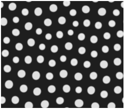
Refer to caption
Figure 1: A multi-droplet pattern: density plot of uu in a local minimizer of ℰ⁡[u]\mathcal{E}[u] with W⁡(u)=14​(1−u2)2W(u)=\tfrac{1}{4}(1-u^{2})^{2} obtained numerically for u¯=−0.5\bar{u}=-0.5, ε=0.025\varepsilon=0.025, and Ω=[0,11.5)×[0,10)\Omega=[0,11.5)\times[0,10), with periodic boundary conditions. Dark regions correspond to u≈−1u\approx-1, and light regions correspond to u≈1u\approx 1 (from [14]).

The parameter ε>0\varepsilon>0 in (1.1) determines both the scale of the short-range interaction and the magnitude of the interfacial energy between the regions with different values of uu when ε\varepsilon is sufficiently small. In fact, it is known that no patterns can form in the system if ε\varepsilon is sufficiently large [13, 14, 38]. On the other hand, when ε≪1\varepsilon\ll 1, the first term in the functional ℰ\mathcal{E} becomes a singular perturbation, giving rise to “domain structures” (see Fig. 1), which are of particular physical interest. These patterns consist of extended regions in which uu is close to one of the minima of the potential WW, separated by narrow domain walls. In this situation one can reduce the energy functional appearing in (1.1) to an expression in terms of the interfaces alone. In [13, 14], such a reduction was performed for ℰ\mathcal{E} using formal asymptotic techniques (see also [39, 40, 30, 35]) and leads to the following reduced energy (for simplicity of notation, we choose the normalizations in such a way that the parameter ε\varepsilon is, in fact, the domain wall energy, see Sec. 4 for details):

E⁡[u]=ε2​∫Ω|∇u|​𝑑x+12​∫Ω∫Ω(u⁡(x)−u¯)​G​(x,y)​(u⁡(y)−u¯)​𝑑x​𝑑y.\displaystyle E[u]={\varepsilon\over 2}\int_{\Omega}|\nabla u|\,dx+\frac{1}{2}\int_{\Omega}\int_{\Omega}(u(x)-\bar{u})G(x,y)(u(y)-\bar{u})\,dx\,dy. (1.4)

Here the function uu takes on values ±1\pm 1 throughout Ω\Omega, and the kernel GG is the screened Coulomb kernel, i.e., it solves the Neumann problem for

−Δ​G​(x,y)+κ2​G​(x,y)=δ⁡(x−y),\displaystyle-\Delta G(x,y)+\kappa^{2}G(x,y)=\delta(x-y), (1.5)

with some κ>0\kappa>0. The constant κ\kappa has the physical meaning of the inverse of the Debye screening length [13, 14]. Note that the sharp interface energy EE with the unscreened Coulomb kernel (i.e. with κ=0\kappa=0) was derived by Ren and Wei as the Γ\Gamma-limit of the diffuse interface energy ℰ\mathcal{E} under assumptions of weak non-local coupling (i.e., with an extra factor of ε\varepsilon in front of the Coulomb kernel) and u¯∈(−1,1)\bar{u}\in(-1,1) independent of ε\varepsilon, as ε→0\varepsilon\to 0 [30] (see also [35]; note that this case is also equivalent to considering ℰ\mathcal{E} on the domain of size O⁡(ε1/3)O(\varepsilon^{1/3})). At the same time, screening becomes important near the transition between the uniform and the patterned states which occurs near |u¯|=1|\bar{u}|=1, the case of interest in the present paper [13, 14]. Note that in the presence of screening the neutrality condition in (1.3) is relaxed.

In this paper, we rigorously establish the relation between the sharp interface energy EE and the diffuse interface energy ℰ\mathcal{E}, and analyze the precise behavior of minimizers of the sharp interface energy EE for ε≪1\varepsilon\ll 1 in the vicinity of the transition from the trivial minimizer to patterned states occurring near |u¯|=1|\bar{u}|=1. We note that despite the apparent simplicity of the expression for EE, the minimizers of EE exhibit quite an intricate dependence on the parameters for ε≪1\varepsilon\ll 1 and |u¯|≃1|\bar{u}|\simeq 1. Our analysis in this paper will be restricted to the case d=2d=2. While a number of our results can be extended to arbitrary space dimensions, our methods to obtain sharp estimates for the energy of minimizers rely critically on the properties of minimal curves in two dimensions and the logarithmic behavior of the Green’s function of the two-dimensional Laplacian near the singularity. Therefore, they cannot be readily extended to other spatial dimensionalities, and, indeed, one would expect certain important differences between these cases and the case of two space dimensions. At the same time, we will show that in the case d=2d=2 it is possible to obtain rather detailed information about the structure of the transition near |u¯|=1|\bar{u}|=1 in terms of energy. Let us note that, since the case d=1d=1 is now well-understood [29, 30, 31, 41], the remaining open case of physical interest is that of d=3d=3.

Before turning to the analysis, let us briefly mention a perfect example of an experimental system in which the regimes studied by us could be easily realized, which is inspired by the beautiful Nobel Lecture of Prof. G. Ertl [42, 43]. Consider molecules which undergo adsorption and desorption to and from a crystalline surface. On the surface, the atoms may hop around and reversibly stick to each other to form monolayer aggregates [44]. Then, within the framework of phase field models, this process may be described by the following evolution equation for the adsorbate density fraction ϕ\phi [25]:

ϕt=M​Δ​(W′​(ϕ)−g​Δ​ϕ)+k+​(1−ϕ)−k−​ϕ,\displaystyle\phi_{t}=M\Delta(W^{\prime}(\phi)-g\Delta\phi)+k_{+}(1-\phi)-k_{-}\phi, (1.6)

where WW is a double-well potential with two minima between ϕ=0\phi=0 and ϕ=1\phi=1, gg is the short-range coupling constant, MM is a kinetic coefficient, and k±k_{\pm} are the adsorption and desorption rates, respectively. Note that this equation can be rewritten as

ϕt=M​Δ​{W′​(ϕ)−g​Δ​ϕ+k​G0∗(ϕ−ϕ¯)},\displaystyle\phi_{t}=M\Delta\{W^{\prime}(\phi)-g\Delta\phi+kG_{0}*(\phi-\bar{\phi})\}, (1.7)

where k=(k++k−)/Mk=(k_{+}+k_{-})/M, ϕ¯=k+/(k++k−)\bar{\phi}=k_{+}/(k_{+}+k_{-}), and “∗*” denotes convolution in space, with G0G_{0} given by (1.2), provided the spatial average of the initial data is ϕ¯\bar{\phi}. Upon suitable rescaling, this is precisely the H−1H^{-1} gradient flow for the energy ℰ\mathcal{E}, i.e., we have ut=Δ⁡(δ​ℰ/δ​u)u_{t}=\Delta(\delta\mathcal{E}/\delta u), where uu is a rescaling of ϕ\phi. In particular, minimizers of ℰ\mathcal{E} are ground states of the considered system in equilibrium in the mean-field limit. We note that the adsorption and desorption rates k±k_{\pm} can be quite small compared to the hopping rate, resulting in very small values of ε∼k1/2\varepsilon\sim k^{1/2}. Therefore, one can achieve a very good scale separation between the interfacial thickness (atomic scales) and the size of adsorbate clusters (micro-scale) in this experimental setup.

Our paper is organized as follows. In Sec. 2, we present heuristic arguments and give the statements of main results, in Sec. 3, we perform a detailed analysis of the sharp interface energy EE, in Sec. 4 we establish a connection between the sharp interface energy EE and the diffuse interface energy ℰ\mathcal{E}. Finally, in Sec. 5 we conclude the proofs of the theorems.

Throughout the paper, the symbols LpL^{p}, HkH^{k}, Wk,pW^{k,p}, Ck,αC^{k,\alpha}, B​VBV denote the usual function spaces, |⋅||\cdot| denotes the dd-dimensional Lebesgue measure or the (d−1)(d-1)-dimensional Hausdorff measure of a set, depending on the context, and CC, cc, etc., denote generic positive constants that can change from line to line. The symbols O⁡(1)O(1) and o⁡(1)o(1) denote, as usual, uniformly bounded and uniformly small quantities, respectively, in the limit ε→0\varepsilon\to 0, etc. Finally, we will say that a statement holds for ε≪1\varepsilon\ll 1, etc., if there exists ε0>0\varepsilon_{0}>0 such that that statement is true for all 0<ε≤ε00<\varepsilon\leq\varepsilon_{0}. For simplicity of notation, the subscript ε\varepsilon is omitted for all quantities depending on ε\varepsilon.

2 Heuristics and main results

Let us begin our investigation by setting d=2d=2 and making a simplifying assumption that the domain Ω\Omega is a torus: Ω=[0,1)2\Omega=[0,1)^{2}. Let us also specify the domains of definition for the functionals ℰ\mathcal{E} and EE. Formally, the diffuse interface energy ℰ⁡[u]\mathcal{E}[u] will be defined for all u∈H1​(Ω)u\in H^{1}(\Omega) subject to ∫Ωu​𝑑x=u¯\int_{\Omega}u\,dx=\bar{u}, whereas the sharp interface energy E⁡[u]E[u] will be defined for all u∈B​V​(Ω,{−1,1})u\in BV(\Omega;\{-1,1\}).

The assumption that Ω\Omega is a torus, which is common in the considered class of problems, eliminates the need to deal with the boundary effects and, even more importantly, restores the translational invariance inherent in the problem on the whole of ℝd\mathbb{R}^{d} (note that the choice of the size of Ω\Omega is inconsequential, the obtained energy of the minimizers scales linearly with |Ω||\Omega|). As a result, the kernel of the non-local part of the energy becomes a function of x−yx-y only. With a slight abuse of notation, in the following we will, therefore, replace G⁡(x,y)G(x,y) with G⁡(x−y)G(x-y) everywhere below.

On heuristic grounds one would expect that the minimizers of EE at ε≪1\varepsilon\ll 1 would be periodic with period R∼ε1/3R\sim\varepsilon^{1/3}, whenever |u¯|<1|\bar{u}|<1 and |u¯||\bar{u}| is not too close to 1 [19, 13, 14, 9]. A simple scaling analysis shows that in this case E∼ε2/3E\sim\varepsilon^{2/3} as ε→0\varepsilon\to 0 with u¯\bar{u} fixed. Our first result gives a justification for this energy scaling without any assumptions about the minimizers (for statements about existence and regularity of minimizers, see the following sections).

Theorem 2.1.

Let WW satisfy the assumptions (i)–(iv) at the beginning of Sec. 4, and let u¯∈(−1,1)\bar{u}\in(-1,1) be fixed. Then there exist ε0>0\varepsilon_{0}>0 and C>c>0C>c>0, such that

c​ε2/3≤min⁡E,min⁡ℰ≤C​ε2/3\displaystyle c\varepsilon^{2/3}\leq\min E,\,\min\mathcal{E}\leq C\varepsilon^{2/3} (2.1)

for all ε≤ε0\varepsilon\leq\varepsilon_{0}.

Observe also that for EE this result still holds when Ω=[0,1)d\Omega=[0,1)^{d} for any dd, while for ℰ\mathcal{E} it holds at least for d<6d<6 (see Sec. 4). We note that for u¯=0\bar{u}=0 and |u|≤1|u|\leq 1 such a result was obtained by Choksi, using somewhat different techniques [9]. On the level of EE (with κ=0\kappa=0), Alberti, Choksi and Otto recently proved, among many other interesting results, a stronger statement that in the limit ε→0\varepsilon\to 0, the constants in the upper and lower bounds in (2.1) can be chosen to be arbitrarily close to each other [36]. We note that the case κ=0\kappa=0 and u¯∈(−1,1)\bar{u}\in(-1,1) fixed can be treated as the limit of energy EE considered by us as κ→0\kappa\to 0, when the constraint ∫Ωu​𝑑x=u¯\int_{\Omega}u\,dx=\bar{u} gets automatically enforced (see (5.2)).

Thus, when u¯∈(−1,1)\bar{u}\in(-1,1) is fixed, the energy EE admits a non-trivial minimizer, whose energy scales as in (2.1) when ε≪1\varepsilon\ll 1. What about the case |u¯|>1|\bar{u}|>1? Here, in fact, it is easy to see that the only minimizers admitted by EE are the trivial ones. Consider, for example, the case u¯<−1\bar{u}<-1, the other case is equivalent by symmetry. In this case the problem admits the unique global minimizer u=−1u=-1. To see this, let us introduce the characteristic function χΩ+\chi_{\Omega^{+}} of the set Ω+={u=+1}\Omega^{+}=\{u=+1\} for a given u∈B​V​(Ω,{−1,1})u\in BV(\Omega;\{-1,1\}). Then u=2​χΩ+−1u=2\chi_{\Omega^{+}}-1, and by a straightforward computation

E⁡[u]\displaystyle E[u] ≥\displaystyle\geq 12​∫Ω∫Ω(2​χΩ+​(x)−1−u¯)​G​(x−y)​(2​χΩ+​(y)−1−u¯)​𝑑x​𝑑y\displaystyle\frac{1}{2}\int_{\Omega}\int_{\Omega}(2\chi_{\Omega^{+}}(x)-1-\bar{u})G(x-y)(2\chi_{\Omega^{+}}(y)-1-\bar{u})dxdy (2.2)
≥\displaystyle\geq (1+u¯)22​κ2−2​(1+u¯)κ2​|Ω+|.\displaystyle{(1+\bar{u})^{2}\over 2\kappa^{2}}-{2(1+\bar{u})\over\kappa^{2}}|\Omega^{+}|.

Thus, when u¯<−1\bar{u}<-1, the second term in the last inequality in (2.2) is positive, hence, is minimized by |Ω+|=0|\Omega^{+}|=0. But in this case u=−1u=-1 attains equality in (2.2), so u=−1u=-1 is the minimizer. Thus, when |u¯|>1|\bar{u}|>1, non-trivial minimizers of EE do not exist, and, therefore, at |u¯|=1|\bar{u}|=1 a bifurcation occurs in the limit ε→0\varepsilon\to 0.

The main purpose of this paper is to investigate the transition between the trivial and the non-trivial minimizers of EE and ℰ\mathcal{E} that occurs in the neighborhood of |u¯|=1|\bar{u}|=1 for ε≪1\varepsilon\ll 1. The energy EE captures most of the difficulty associated with the considered problem. Therefore, we will spend most of our effort in this paper to the studies of EE (see Sec. 3). At the same time, as we show later (see Sec. 4), the statements about the behavior of min⁡E\min E also extend to that of min⁡ℰ\min\mathcal{E} for ε≪1\varepsilon\ll 1 (the correspondence of minimizers of the two energies will be a subject of future study).

When Ω=[0,1)2\Omega=[0,1)^{2}, the kernel GG has an explicit representation

G⁡(x)=12​π​∑𝐧∈ℤ2K0​(κ​|x−𝐧|),\displaystyle G(x)=\frac{1}{2\pi}\sum_{\mathbf{n}\in\mathbb{Z}^{2}}K_{0}(\kappa|x-\mathbf{n}|), (2.3)

where K0K_{0} is the modified Bessel function of the first kind. In particular, G>0G>0 and we have the following asymptotic expansion from the power series representation of K0K_{0} [45]:

G⁡(x)=−12​π​ln⁡(κ¯​|x|)+O⁡(|x|),|x|≪1,\displaystyle G(x)=-\frac{1}{2\pi}\ln(\bar{\kappa}|x|)+O(|x|),\qquad|x|\ll 1, (2.4)

where

κ¯=12​κ​exp⁡(γ−∑𝐧∈ℤ2\{0}K0​(κ​|𝐧|)),\displaystyle\bar{\kappa}=\tfrac{1}{2}\kappa\exp\left(\gamma-\sum_{\mathbf{n}\in\mathbb{Z}^{2}\backslash\{0\}}K_{0}(\kappa|\mathbf{n}|)\right), (2.5)

and γ≈0.5772\gamma\approx 0.5772 is the Euler’s constant. We also have G⁡(x)G(x) bounded whenever |x|>δ|x|>\delta, for any δ>0\delta>0, and (2.4) can be used to estimate derivatives of GG to O⁡(|x|​ln⁡|x|)O(|x|\ln|x|) as well.

Consider the case in which the value of u¯\bar{u} approaches u¯=−1\bar{u}=-1 from above, with ε≪1\varepsilon\ll 1 fixed. Clearly, for large enough deviations there exists a non-trivial minimizer. As can be seen from the arguments in the proof of Theorem 2.1, the size of the set where u=1u=1 on the minimizer goes to zero as u¯→−1\bar{u}\to-1. Heuristically, one would, therefore, expect that in this situation the minimizer will consist of a number of isolated droplets where u=+1u=+1 of small size in the background where u=−1u=-1. Moreover, since on the scale of a droplet the interfacial energy will give a dominant contribution, these droplets are expected to be nearly circular. This motivates an introduction of the following reduced energy:

EN​({ri},{xi})\displaystyle E_{N}(\{r_{i}\},\{x_{i}\}) =\displaystyle= ∑i=1N(2​π​ε​ri−2​π​(1+u¯)​κ−2​ri2−π​ri4​(ln⁡κ¯​ri−14))\displaystyle\sum_{i=1}^{N}\Bigl(2\pi\varepsilon r_{i}-2\pi(1+\bar{u})\kappa^{-2}r_{i}^{2}-\pi r_{i}^{4}(\ln\bar{\kappa}r_{i}-\tfrac{1}{4})\Bigr) (2.6)
+\displaystyle+ 4​π2​∑i=1N−1∑j=i+1NG⁡(xi−xj)​ri2​rj2.\displaystyle 4\pi^{2}\sum_{i=1}^{N-1}\sum_{j=i+1}^{N}G(x_{i}-x_{j})r_{i}^{2}r_{j}^{2}.

which describes the energy of interaction of NN well separated disk-shaped droplets of radius rir_{i} centered at xix_{i}, to the leading order. More precisely, the first term (2.6) stands for the interfacial energy of all the droplets, the second term is the energy of interactions between the droplets and the background, the third term is the self-interaction energy of each droplet, and the last term is the interaction energy of each droplet pair (for the case of a single droplet in ℝ2\mathbb{R}^{2}, see [14]).

We can use the reduced energy in (2.6) to obtain the leading order scaling of various quantities for ε≪1\varepsilon\ll 1 by balancing different terms. From the balance of interfacial energy and the self-interaction energy, one should have ri=O(ε1/3|lnε|−1/3)r_{i}=O(\varepsilon^{1/3}|\ln\varepsilon|^{-1/3}). Balancing this with the second term leads, in turn, to

δ¯=ε−2/3|lnε|−1/3(1+u¯)\displaystyle\bar{\delta}=\varepsilon^{-2/3}|\ln\varepsilon|^{-1/3}(1+\bar{u}) (2.7)

being an O⁡(1)O(1) quantity. Similarly, balancing the last term with the first three leads to N=O⁡(|ln⁡ε|)N=O(|\ln\varepsilon|), and the expected behavior of min⁡EN=O⁡(ε4/3​|ln⁡ε|2/3)\min E_{N}=O(\varepsilon^{4/3}|\ln\varepsilon|^{2/3}). One would also expect that, since the droplets repel each other, in a minimum energy configuration they would become uniformly distributed throughout Ω\Omega.

Our main result proves and further quantifies this heuristic picture on the level of the sharp interface energy EE.

Theorem 2.2.

Let u¯=−1+ε2/3​|ln⁡ε|1/3​δ¯\bar{u}=-1+\varepsilon^{2/3}|\ln\varepsilon|^{1/3}\bar{\delta}, with some δ¯>0\bar{\delta}>0 fixed. Then for any σ>0\sigma>0 sufficiently small there exists ε0>0\varepsilon_{0}>0 such that for all ε≤ε0\varepsilon\leq\varepsilon_{0}:

  • (i)

    If δ¯<12​93​κ2\bar{\delta}<\tfrac{1}{2}\sqrt[3]{9}\,\kappa^{2}, then u=−1u=-1 is the unique global minimizer of EE, with ε−4/3|lnε|−2/3minE=12κ−2δ¯2\varepsilon^{-4/3}|\ln\varepsilon|^{-2/3}\min E=\tfrac{1}{2}\kappa^{-2}\bar{\delta}^{2}.

  • (ii)

    If δ¯>12​93​κ2\bar{\delta}>\tfrac{1}{2}\sqrt[3]{9}\,\kappa^{2}, there exists a non-trivial minimizer of EE. The minimizer is

    u⁡(x)=−1+2​∑i=1NχΩi+​(x),\displaystyle u(x)=-1+2\sum_{i=1}^{N}\chi_{\Omega^{+}_{i}}(x), (2.8)

    where χΩi+\chi_{\Omega^{+}_{i}} are characteristic functions of NN disjoint simply connected sets Ωi+⊂Ω\Omega^{+}_{i}\subset\Omega with boundary of class C3C^{3}, and N=O⁡(|ln⁡ε|)N=O(|\ln\varepsilon|). The boundary of each set Ωi+\Omega^{+}_{i} is O⁡(ε2/3−σ)O(\varepsilon^{2/3-\sigma})-close (in Hausdorff sense) to a circle of radius rir_{i} centered at xix_{i}. Furthermore,

    min⁡E=12​ε4/3​|ln⁡ε|2/3​κ−2​δ¯2+EN​({ri},{xi})+O⁡(ε5/3−σ),\displaystyle\min E=\tfrac{1}{2}\varepsilon^{4/3}|\ln\varepsilon|^{2/3}\kappa^{-2}\bar{\delta}^{2}+E_{N}(\{r_{i}\},\{x_{i}\})+O(\varepsilon^{5/3-\sigma}), (2.9)

    with EN=O⁡(ε4/3​|ln⁡ε|2/3)E_{N}=O(\varepsilon^{4/3}|\ln\varepsilon|^{2/3}), ri=O(ε1/3|lnε|−1/3)r_{i}=O(\varepsilon^{1/3}|\ln\varepsilon|^{-1/3}), and

    |xi−xj|>εσ,∀j≠i.\displaystyle|x_{i}-x_{j}|>\varepsilon^{\sigma},\quad\forall j\not=i. (2.10)
  • (iii)

    If δ¯>12​93​κ2\bar{\delta}>\tfrac{1}{2}\sqrt[3]{9}\,\kappa^{2}, in the limit ε→0\varepsilon\to 0 we have

    ε−1/3|lnε|1/3ri\displaystyle\varepsilon^{-1/3}|\ln\varepsilon|^{1/3}r_{i} →\displaystyle\to 33\displaystyle\sqrt[3]{3} (2.11)

    uniformly,

    1|ln⁡ε|​∑i=1Nδ⁡(x−xi)\displaystyle{1\over|\ln\varepsilon|}\sum_{i=1}^{N}\delta(x-x_{i}) →\displaystyle\to 12​π​93​(δ¯−932​κ2),\displaystyle{1\over 2\pi\sqrt[3]{9}}\left(\bar{\delta}-{\sqrt[3]{9}\over 2}\,\kappa^{2}\right), (2.12)

    weakly in the sense of measures, and

    ε−4/3|lnε|−2/3minE\displaystyle\varepsilon^{-4/3}|\ln\varepsilon|^{-2/3}\min E →\displaystyle\to 932​(δ¯−934​κ2).\displaystyle{\sqrt[3]{9}\over 2}\left(\bar{\delta}-{\sqrt[3]{9}\over 4}\,\kappa^{2}\right). (2.13)

Note that a more detailed result on the structure of the transition occurring near δ¯=12​93​κ2\bar{\delta}=\tfrac{1}{2}\sqrt[3]{9}\,\kappa^{2} is presented in Proposition 3.20.

Let us make a few remarks related to the statements of Theorem 2.2. For small, but finite values of ε\varepsilon this theorem establishes an equivalence between the sharp interface energy EE and the energy of NN interacting droplets ENE_{N}, in the sense that the minimizers of EE are close to “almost” minimizers of ENE_{N}, i.e., we have EN<min⁡EN+O⁡(ε5/3−σ)E_{N}<\min E_{N}+O(\varepsilon^{5/3-\sigma}). Nevertheless, to prove closeness of minimizers of EE to those of ENE_{N} we also need some coercivity of the energy ENE_{N}. This problem has to do with the properties of the minimizers of the pairwise interaction of the droplets, i.e. the choice of xix_{i} which minimize ENE_{N} with fixed rir_{i}. This becomes a difficult problem in the case of interest, since we generally expect N≫1N\gg 1 (for a numerical solution at a few values of NN and κ=2\kappa=2 see Fig. 2). It would be natural to conjecture that at small enough ε\varepsilon the minimizing droplets will arrange themselves into a periodic lattice close to a hexagonal (close-packed) lattice. Proving this kind of result, however, is a major challenge (see [46] for a recent proof for a certain class of pair interactions), which is one of the open questions also in many other problems, such as the problem of characterizing Abrikosov vortex lattices, for example [47]. Let us mention here a recent result by Chen and Oshita, who proved that in the case κ=0\kappa=0 the hexagonal arrangement of disks is energetically the best among simple periodic lattices [48]. Yet, it is not known if the same result also holds for more general arrangements of droplets. Here we prove a weaker result that the number density of droplets becomes asymptotically uniform as ε→0\varepsilon\to 0, leading also to uniform distribution of energy (compare with [36]). Moreover, we identify the precise asymptotic behavior of the minimal energy and the size of the minimizing droplets as ε→0\varepsilon\to 0.

Figure 2: “Coulombic dice”: Minimizers of ENE_{N} with ri=33ε1/3|lnε|−1/3r_{i}=\sqrt[3]{3}\,\varepsilon^{1/3}|\ln\varepsilon|^{-1/3} for κ=2\kappa=2 and N=2,3,4,5N=2,3,4,5, obtained using random search algorithm.

Lastly, we establish the asymptotic behavior of the minimal value of the diffuse interface energy ℰ\mathcal{E} (which, of course, agrees with the result for the sharp interface energy).

Theorem 2.3.

Let WW satisfy assumptions (i)–(iv) at the beginning of Sec. 4, let u¯=−1+ε2/3​|ln⁡ε|1/3​δ¯\bar{u}=-1+\varepsilon^{2/3}|\ln\varepsilon|^{1/3}\bar{\delta}, with some δ¯>0\bar{\delta}>0 fixed, and let κ\kappa be given by (4.10). Then

  • (i)

    If δ¯≤12​93​κ2\bar{\delta}\leq\tfrac{1}{2}\sqrt[3]{9}\,\kappa^{2}, then ε−4/3|lnε|−2/3minℰ→12κ−2δ¯2\varepsilon^{-4/3}|\ln\varepsilon|^{-2/3}\min\mathcal{E}\to\tfrac{1}{2}\kappa^{-2}\bar{\delta}^{2},

  • (ii)

    If δ¯>12​93​κ2\bar{\delta}>\tfrac{1}{2}\sqrt[3]{9}\,\kappa^{2}, then ε−4/3|lnε|−2/3minℰ→932(δ¯−934κ2)\varepsilon^{-4/3}|\ln\varepsilon|^{-2/3}\min\mathcal{E}\to{\sqrt[3]{9}\over 2}\left(\bar{\delta}-{\sqrt[3]{9}\over 4}\,\kappa^{2}\right),

as ε→0\varepsilon\to 0.

The proofs of Theorems 2.1–2.3 are based on a number of propositions established in Secs. 3 and 4, and are completed in Sec. 5.

3 Analysis of the sharp interface problem

Our plan for the analysis of the sharp interface problem consists of a number of steps which we list below:

  1. 1.

    Introduce a suitably rescaled energy E¯\bar{E} and domain Ω¯\bar{\Omega}.

  2. 2.

    Establish existence and regularity of the minimizers of E¯\bar{E} (subsets of Ω¯\bar{\Omega} where u=1u=1).

  3. 3.

    Establish some a priori estimates for the geometry of the minimizers of E¯\bar{E} and uniform bounds on the induced long-range potential.

  4. 4.

    Establish that different connected components of minimizers of E¯\bar{E} are separated by large distances in Ω¯\bar{\Omega}.

  5. 5.

    Establish that each connected component of a minimizer of E¯\bar{E} is close to a disk (hence the term “droplet”).

  6. 6.

    Establish equivalence between min⁡E¯\min\bar{E} and min⁡E¯N\min\bar{E}_{N} (the suitably rescaled version of ENE_{N}).

  7. 7.

    Improve the estimate for the separation distance between different droplets.

  8. 8.

    Prove uniform convergence of the rescaled droplet radii to a universal constant.

  9. 9.

    Prove convergence of min⁡E¯\min\bar{E} to a limit and convergence of the normalized droplet density in the original, unscaled domain Ω\Omega to a limit, as ε→0\varepsilon\to 0.

This plan is carried out in the rest of this section via a series of lemmas and propositions.

3.1 Scaling

We begin by introducing a suitable rescaling, in which the main quantities of interest become O⁡(1)O(1) quantities in the limit ε→0\varepsilon\to 0. Motivated by the discussion of Sec. 2, we define the rescaled energy E¯\bar{E} (with the energy of the uniform state u=−1u=-1 subtracted) and a new coordinate x¯∈Ω¯=[0,ε1/3|lnε|−1/3)2\bar{x}\in\bar{\Omega}=[0,\varepsilon^{1/3}|\ln\varepsilon|^{-1/3})^{2}, where Ω¯\bar{\Omega} is a two-dimensional torus with period ε1/3|lnε|−1/3\varepsilon^{1/3}|\ln\varepsilon|^{-1/3}:

E=ε4/3​|ln⁡ε|2/3​(12​κ−2​δ¯2+E¯),x=ε1/3|ln⁡ε|1/3​x¯.\displaystyle E=\varepsilon^{4/3}|\ln\varepsilon|^{2/3}\,(\tfrac{1}{2}\kappa^{-2}\bar{\delta}^{2}+\bar{E}),\qquad x={\varepsilon^{1/3}\over|\ln\varepsilon|^{1/3}}\,\bar{x}. (3.1)

The energy E¯\bar{E} can be conveniently expressed in term of the set Ω¯+⊂Ω¯\bar{\Omega}^{+}\subset\bar{\Omega} in which u=1u=1:

E¯\displaystyle\bar{E} =\displaystyle= |ln⁡ε|−1​(|∂Ω¯+|−2​δ¯​κ−2​|Ω¯+|)\displaystyle|\ln\varepsilon|^{-1}\bigl(|\partial\bar{\Omega}^{+}|-2\bar{\delta}\kappa^{-2}|\bar{\Omega}^{+}|\bigr) (3.2)
+\displaystyle+ 2|lnε|−2∫Ω¯+∫Ω¯+G(ε1/3|lnε|−1/3(x¯−y¯))dx¯dy¯.\displaystyle 2|\ln\varepsilon|^{-2}\int_{\bar{\Omega}^{+}}\int_{\bar{\Omega}^{+}}G\bigl(\varepsilon^{1/3}|\ln\varepsilon|^{-1/3}(\bar{x}-\bar{y})\bigr)d\bar{x}\,d\bar{y}.

We also need an expression for the rescaled energy E¯N\bar{E}_{N} of a system of interacting droplets. With the help of (3.1), we can write the rescaling of (2.6) as

E¯N\displaystyle\bar{E}_{N} =\displaystyle= 2​π|ln⁡ε|∑i=1N{r¯i−δ¯κ−2r¯i2−12|lnε|−1r¯i4(ln(ε1/3|lnε|−1/3κ¯r¯i)−14)}\displaystyle{2\pi\over|\ln\varepsilon|}\sum_{i=1}^{N}\left\{\bar{r}_{i}-\bar{\delta}\kappa^{-2}\,\bar{r}_{i}^{2}-\tfrac{1}{2}|\ln\varepsilon|^{-1}\bar{r}_{i}^{4}\left(\ln(\varepsilon^{1/3}|\ln\varepsilon|^{-1/3}\bar{\kappa}\bar{r}_{i})-\tfrac{1}{4}\right)\right\} (3.3)
+\displaystyle+ 4​π2|ln⁡ε|2∑i=1N−1∑j=i+1NG(ε1/3|lnε|−1/3(x¯i−x¯j))r¯i2r¯j2,\displaystyle{4\pi^{2}\over|\ln\varepsilon|^{2}}\sum_{i=1}^{N-1}\sum_{j=i+1}^{N}G(\varepsilon^{1/3}|\ln\varepsilon|^{-1/3}(\bar{x}_{i}-\bar{x}_{j}))\bar{r}_{i}^{2}\bar{r}_{j}^{2},

where r¯i\bar{r}_{i} and x¯i\bar{x}_{i} are the radii and the centers of the droplets, respectively.

3.2 Properties of minimizers

Let us begin with the statement of a result on the existence and regularity of minimizers of E¯\bar{E} (or, equivalently, of EE), which is obtained by straightforwardly adapting the results of [49] for sets of prescribed mean curvature.

Proposition 3.1.

There exists a set Ω¯+\bar{\Omega}^{+} of finite perimeter which minimizes E¯\bar{E} in (3.2). The boundary ∂Ω¯+\partial\bar{\Omega}^{+} of this set is a curve of class C1,αC^{1,\alpha} for some α∈(0,1)\alpha\in(0,1).

In view of this, in the following we will always assume that minimizers Ω¯+\bar{\Omega}^{+} of E¯\bar{E} are closed sets. We also note that

v(x¯)=|lnε|−1∫Ω¯+G(ε1/3|lnε|−1/3(x¯−y¯))dy¯\displaystyle v(\bar{x})=|\ln\varepsilon|^{-1}\int_{\bar{\Omega}^{+}}G(\varepsilon^{1/3}|\ln\varepsilon|^{-1/3}(\bar{x}-\bar{y}))\,d\bar{y} (3.4)

is in W2,p​(Ω¯)W^{2,p}(\bar{\Omega}), with any p>1p>1, and, hence, in C1,α​(Ω¯)C^{1,\alpha}(\bar{\Omega}) for any α∈(0,1)\alpha\in(0,1). Indeed, v¯\bar{v} solves the equation

−Δv+ε2/3|lnε|−2/3κ2v=|lnε|−1χΩ¯+,\displaystyle-\Delta v+\varepsilon^{2/3}|\ln\varepsilon|^{-2/3}\kappa^{2}v=|\ln\varepsilon|^{-1}\chi_{\bar{\Omega}^{+}}, (3.5)

where χΩ¯+\chi_{\bar{\Omega}^{+}} is the characteristic function of Ω¯+\bar{\Omega}^{+}, in Ω¯\bar{\Omega}, and so the result follows by standard elliptic regularity theory [50]. As a consequence, we have a higher regularity for the boundary of the minimizer Ω¯+\bar{\Omega}^{+} of E¯\bar{E} ([51], see also [35]):

Corollary 3.2.

The boundary ∂Ω¯+\partial\bar{\Omega}^{+} of a minimizer Ω¯+\bar{\Omega}^{+} of E¯\bar{E} is of class C3,αC^{3,\alpha}.

Note that this regularity result also holds more generally for local minimizers of E¯\bar{E} in dimensions d≤7d\leq 7 [49], hence, in particular, the expressions for the first and second variation of E¯\bar{E} in d≤3d\leq 3 obtained in [14] are justified (see also [52] for the case of arbitrary dimensions). If ρ∈C1​(∂Ω¯)\rho\in C^{1}(\partial\bar{\Omega}), a>0a>0, and Ω¯a\bar{\Omega}_{a} is the set obtained by displacing ∂Ω¯+\partial\bar{\Omega}^{+} by a​ρa\rho in the outward normal direction, then a↦E¯​(Ω¯a+)a\mapsto\bar{E}(\bar{\Omega}^{+}_{a}) is twice continuously differentiable at a=0a=0, and we have [14] (for the reader’s convenience, the computation is reproduced in Appendix C):

|ln⁡ε|​d​E¯​(Ω¯a+)d​a|a=0=∫∂Ω¯+(K⁡(x¯)−2​δ¯​κ−2+4​v​(x¯))​ρ​(x¯)​d​ℋ1​(x¯),\displaystyle|\ln\varepsilon|\left.{d\bar{E}(\bar{\Omega}^{+}_{a})\over da}\right|_{a=0}=\int_{\partial\bar{\Omega}^{+}}(K(\bar{x})-2\bar{\delta}\kappa^{-2}+4v(\bar{x}))\rho(\bar{x})\,d\mathcal{H}^{1}(\bar{x}), (3.6)
|ln⁡ε|​d2​E¯​(Ω¯a+)d​a2|a=0=∫∂Ω¯+(|∇ρ​(x¯)|2+4​ν​(x¯)⋅∇v​(x¯)​ρ2​(x¯))​d​ℋ1​(x¯)\displaystyle|\ln\varepsilon|\left.{d^{2}\bar{E}(\bar{\Omega}^{+}_{a})\over da^{2}}\right|_{a=0}=\int_{\partial\bar{\Omega}^{+}}\bigl(|\nabla\rho(\bar{x})|^{2}+4\nu(\bar{x})\cdot\nabla v(\bar{x})\,\rho^{2}(\bar{x})\bigr)\,d\mathcal{H}^{1}(\bar{x})
+∫∂Ω¯+(4v(x¯)−2δ¯κ−2)K(x¯)ρ2(x¯)dℋ1(x¯)\displaystyle+\int_{\partial\bar{\Omega}^{+}}(4v(\bar{x})-2\bar{\delta}\kappa^{-2})K(\bar{x})\rho^{2}(\bar{x})\,d\mathcal{H}^{1}(\bar{x})
+4|lnε|−1∫∂Ω¯+∫∂Ω¯+G(ε1/3|lnε|−1/3(x¯−y¯))ρ(x¯)ρ(y¯)dℋ1(x¯)dℋ1(y¯).\displaystyle+4|\ln\varepsilon|^{-1}\int_{\partial\bar{\Omega}^{+}}\int_{\partial\bar{\Omega}^{+}}G(\varepsilon^{1/3}|\ln\varepsilon|^{-1/3}(\bar{x}-\bar{y}))\rho(\bar{x})\rho(\bar{y})\,d\mathcal{H}^{1}(\bar{x})d\mathcal{H}^{1}(\bar{y}). (3.7)

where K⁡(x¯)K(\bar{x}) is the curvature at point x¯∈∂Ω¯+\bar{x}\in\partial\bar{\Omega}^{+}, with the sign convention that K>0K>0 if Ω¯+\bar{\Omega}^{+} is convex, and ν⁡(x¯)\nu(\bar{x}) is the outward unit normal to ∂Ω¯+\partial\bar{\Omega}^{+} at that point. The associated Euler-Lagrange equation for ∂Ω¯+\partial\bar{\Omega}^{+} reads

K⁡(x¯)=2​δ¯​κ−2−4​v​(x¯),\displaystyle K(\bar{x})=2\bar{\delta}\kappa^{-2}-4v(\bar{x}), (3.8)

which also allows to simplify the expression in (3.7) evaluated on a minimizer to

|ln⁡ε|​d2​E¯​(Ω¯a+)d​a2|a=0=\displaystyle|\ln\varepsilon|\left.{d^{2}\bar{E}(\bar{\Omega}^{+}_{a})\over da^{2}}\right|_{a=0}=\hskip 184.9429pt
∫∂Ω¯+(|∇ρ​(x¯)|2+4​ν​(x¯)⋅∇v​(x¯)​ρ2​(x¯)−K2​(x¯)​ρ2​(x¯))​d​ℋ1​(x¯)\displaystyle\int_{\partial\bar{\Omega}^{+}}\bigl(|\nabla\rho(\bar{x})|^{2}+4\nu(\bar{x})\cdot\nabla v(\bar{x})\,\rho^{2}(\bar{x})-K^{2}(\bar{x})\rho^{2}(\bar{x})\bigr)\,d\mathcal{H}^{1}(\bar{x})
+4|lnε|−1∫∂Ω¯+∫∂Ω¯+G(ε1/3|lnε|−1/3(x¯−y¯))ρ(x¯)ρ(y¯)dℋ1(x¯)dℋ1(y¯).\displaystyle+4|\ln\varepsilon|^{-1}\int_{\partial\bar{\Omega}^{+}}\int_{\partial\bar{\Omega}^{+}}G(\varepsilon^{1/3}|\ln\varepsilon|^{-1/3}(\bar{x}-\bar{y}))\rho(\bar{x})\rho(\bar{y})\,d\mathcal{H}^{1}(\bar{x})d\mathcal{H}^{1}(\bar{y}). (3.9)

We will use these equations later on to establish some properties of the minimizers for ε≪1\varepsilon\ll 1. Meanwhile, let us begin our analysis with some basic estimates.

Lemma 3.3.

Let Ω¯+\bar{\Omega}^{+} be a minimizer of E¯\bar{E}. Then there exists C>0C>0 such that

|Ω¯+|\displaystyle|\bar{\Omega}^{+}| ≤\displaystyle\leq C​|ln⁡ε|,\displaystyle C|\ln\varepsilon|, (3.10)
|∂Ω¯+|\displaystyle|\partial\bar{\Omega}^{+}| ≤\displaystyle\leq C​|ln⁡ε|.\displaystyle C|\ln\varepsilon|. (3.11)

for ε≪1\varepsilon\ll 1.

Proof.

First of all, by representation (2.3) we have G⁡(x−y)≥c>0G(x-y)\geq c>0 for all x,y∈Ωx,y\in\Omega. Therefore, in view of the fact that min⁡E¯≤0\min\bar{E}\leq 0 (since E¯=0\bar{E}=0 if Ω¯+=∅\bar{\Omega}^{+}=\varnothing), from (3.2) we have

0≥|ln⁡ε|​E¯\displaystyle 0\geq|\ln\varepsilon|\,\bar{E} ≥\displaystyle\geq 2|lnε|−1∫Ω¯+∫Ω¯+G(ε1/3|lnε|−1/3(x¯−y¯))dx¯−2δ¯κ−2|Ω¯+|\displaystyle 2|\ln\varepsilon|^{-1}\int_{\bar{\Omega}^{+}}\int_{\bar{\Omega}^{+}}G\bigl(\varepsilon^{1/3}|\ln\varepsilon|^{-1/3}(\bar{x}-\bar{y})\bigr)d\bar{x}-2\bar{\delta}\kappa^{-2}|\bar{\Omega}^{+}| (3.12)
≥\displaystyle\geq 2​c​|ln⁡ε|−1​|Ω¯+|2−2​δ¯​κ−2​|Ω¯+|,\displaystyle 2c|\ln\varepsilon|^{-1}\,|\bar{\Omega}^{+}|^{2}-2\bar{\delta}\kappa^{-2}|\bar{\Omega}^{+}|,

which gives (3.10). On the other hand, we also have

|∂Ω¯+|≤2​δ¯​κ−2​|Ω¯+|.\displaystyle|\partial\bar{\Omega}^{+}|\leq 2\bar{\delta}\kappa^{-2}|\bar{\Omega}^{+}|. (3.13)

Therefore, from (3.10) we immediately obtain (3.11). ∎

As a corollary, it follows from (3.11) that the diameter of each connected subset Ω¯i+\bar{\Omega}^{+}_{i} of Ω¯+\bar{\Omega}^{+} is bounded by O⁡(|ln⁡ε|)O(|\ln\varepsilon|)

diam⁡(Ω¯i+)≤C​|ln⁡ε|,\displaystyle\mathrm{diam}(\bar{\Omega}^{+}_{i})\leq C|\ln\varepsilon|, (3.14)

for some C>0C>0 independent of ε≪1\varepsilon\ll 1.

Our next step is to show that the area of each connected component of Ω¯+≠∅\bar{\Omega}^{+}\not=\varnothing is uniformly bounded above and below independently of ε\varepsilon.

Lemma 3.4.

Let Ω¯+=∪i=1NΩ¯+i\bar{\Omega}^{+}=\cup_{i=1}^{N}\bar{\Omega}^{+}_{i} be a non-trivial minimizer of E¯\bar{E}, where Ω¯i+\bar{\Omega}^{+}_{i} are the disjoint connected components of Ω¯+\bar{\Omega}^{+}. Then, there exist C>c>0C>c>0 such that

c≤|Ω¯i+|,|∂Ω¯i+|≤C,diam⁡(Ω¯i+)≤C,\displaystyle c\leq|\bar{\Omega}^{+}_{i}|,|\partial\bar{\Omega}^{+}_{i}|\leq C,\qquad\mathrm{diam}(\bar{\Omega}^{+}_{i})\leq C, (3.15)

for ε≪1\varepsilon\ll 1.

Proof.

First, note that since by Corollary 3.2 the set ∂Ω¯+\partial\bar{\Omega}^{+} is of class C3,αC^{3,\alpha} we have N<∞N<\infty. To see that (3.15) holds, we first write E¯\bar{E} as

|ln⁡ε|​E¯\displaystyle|\ln\varepsilon|\,\bar{E} =\displaystyle= ∑i=1N(|∂Ω¯i+|−2​δ¯​κ−2​|Ω¯i+|CLOSE\displaystyle\sum_{i=1}^{N}\Biggl(|\partial\bar{\Omega}^{+}_{i}|-2\bar{\delta}\kappa^{-2}|\bar{\Omega}^{+}_{i}| (3.16)
+\displaystyle+ 2|lnε|−1∫Ω¯i+∫Ω¯i+G(ε1/3|lnε|−1/3(x¯−y¯))dx¯dy¯\displaystyle 2|\ln\varepsilon|^{-1}\int_{\bar{\Omega}^{+}_{i}}\int_{\bar{\Omega}^{+}_{i}}G(\varepsilon^{1/3}|\ln\varepsilon|^{-1/3}(\bar{x}-\bar{y}))\,d\bar{x}d\bar{y}
+\displaystyle+ 2|lnε|−1∑j≠i∫Ω¯i+∫Ω¯j+G(ε1/3|lnε|−1/3(x¯−y¯))dx¯dy¯).\displaystyle 2|\ln\varepsilon|^{-1}\sum_{j\not=i}\int_{\bar{\Omega}^{+}_{i}}\int_{\bar{\Omega}^{+}_{j}}G(\varepsilon^{1/3}|\ln\varepsilon|^{-1/3}(\bar{x}-\bar{y}))\,d\bar{x}d\bar{y}\Biggr).

In view of (3.14) and (2.4), the integral in the second line in (3.16) is bounded from below by 16​π​(1−δ)​|ln⁡ε|​|Ω¯i+|2\tfrac{1}{6\pi}(1-\delta)|\ln\varepsilon|\,|\bar{\Omega}^{+}_{i}|^{2} for any δ>0\delta>0, provided ε\varepsilon is small enough. Therefore, removing the set Ω¯i+\bar{\Omega}^{+}_{i} from Ω¯+\bar{\Omega}^{+} will result in the change of energy Δ​E¯\Delta\bar{E} estimated as

|ln⁡ε|​Δ​E¯\displaystyle|\ln\varepsilon|\,\Delta\bar{E} ≤\displaystyle\leq −(|∂Ω¯i+|−2​δ¯​κ−2​|Ω¯i+|+13​π​(1−δ)​|Ω¯i+|2)\displaystyle-\biggl(|\partial\bar{\Omega}^{+}_{i}|-2\bar{\delta}\kappa^{-2}|\bar{\Omega}^{+}_{i}|+\tfrac{1}{3\pi}(1-\delta)|\bar{\Omega}^{+}_{i}|^{2}\biggr) (3.17)
≤\displaystyle\leq −(2​π​|Ω¯i+|1/2−2​δ¯​κ−2​|Ω¯i+|+13​π​(1−δ)​|Ω¯i+|2),\displaystyle-\biggl(2\sqrt{\pi}\,|\bar{\Omega}^{+}_{i}|^{1/2}-2\bar{\delta}\kappa^{-2}|\bar{\Omega}^{+}_{i}|+\tfrac{1}{3\pi}(1-\delta)|\bar{\Omega}^{+}_{i}|^{2}\biggr),

where in the first line we took into account that G>0G>0 and in the second line used the isoperimetric inequality. Then, by direct inspection (see also Fig. 3) we have Δ​E¯<0\Delta\bar{E}<0, contradicting minimality of E¯\bar{E} on Ω¯+\bar{\Omega}^{+}, unless c≤|Ω¯i+|≤Cc\leq|\bar{\Omega}^{+}_{i}|\leq C for some C>c>0C>c>0, independently of ε≪1\varepsilon\ll 1. Finally, the lower bound for |∂Ω¯i+||\partial\bar{\Omega}^{+}_{i}| follows from the isoperimetric inequality, and the upper bound is obtained by applying the previous argument to the first line in (3.17). ∎

Figure 3: The graph of V0​(r¯)V_{0}(\bar{r}) from (3.18) for different values of δ¯\bar{\delta}.

Following the same arguments, we also immediately arrive at the following non-existence result:

Proposition 3.5.

Let δ¯<12​93​κ2\bar{\delta}<\tfrac{1}{2}\sqrt[3]{9}\,\kappa^{2} be fixed. Then the unique minimizer of E¯\bar{E} is Ω¯+=∅\bar{\Omega}^{+}=\varnothing for ε≪1\varepsilon\ll 1.

Proof.

Let us introduce the function Vv:[0,∞)→ℝV_{v}:[0,\infty)\to\mathbb{R}, defined as

Vv​(r¯)=2​π​(r¯+(2​v−δ¯​κ−2)​r¯2+16​r¯4),\displaystyle V_{v}(\bar{r})=2\pi\left(\bar{r}+(2v-\bar{\delta}\kappa^{-2})\bar{r}^{2}+\tfrac{1}{6}\bar{r}^{4}\right), (3.18)

whose graph at v=0v=0 and several values of δ¯\bar{\delta} is shown in Fig. 3. If Ω¯i+\bar{\Omega}^{+}_{i} is a connected component of Ω¯+\bar{\Omega}^{+} and r¯i=(1π​|Ω¯i+|)1/2\bar{r}_{i}=(\tfrac{1}{\pi}|\bar{\Omega}^{+}_{i}|)^{1/2}, then by the same arguments as in Lemma 3.4, the energy gained by removing Ω¯i+\bar{\Omega}^{+}_{i} from Ω¯+\bar{\Omega}^{+} is bounded below by |ln⁡ε|−1​(V0​(r¯i)+o⁡(1))|\ln\varepsilon|^{-1}(V_{0}(\bar{r}_{i})+o(1)), as long as ε≪1\varepsilon\ll 1. Then, by direct inspection V0​(r¯)V_{0}(\bar{r}) is always positive under the assumptions of the proposition, making Ω¯+=∅\bar{\Omega}^{+}=\varnothing energetically preferred. ∎

Note that the asymptotic value of the threshold of δ¯\bar{\delta} in Proposition 3.5 below which no non-trivial minimizers are present was computed in [14]. Another simple corollary to Proposition 3.4 is the following

Lemma 3.6.

Let Ω¯+\bar{\Omega}^{+} be a non-trivial minimizer of E¯\bar{E} and let NN be the number of disjoint connected components of Ω¯+\bar{\Omega}^{+}. Then there exists C>0C>0 such that

N≤C​|ln⁡ε|,\displaystyle N\leq C|\ln\varepsilon|, (3.19)

for ε≪1\varepsilon\ll 1.

Let us now establish a uniform bound on the potential vv. Note that a version of this result is also an important component in the proofs of [36].

Lemma 3.7.

Let Ω¯+\bar{\Omega}^{+} be a non-trivial minimizer of E¯\bar{E}. Then for any α∈(0,1)\alpha\in(0,1) we have

0<v≤C,‖v‖C1,α​(Ω¯)≤C,\displaystyle 0<v\leq C,\qquad||v||_{C^{1,\alpha}(\bar{\Omega})}\leq C, (3.20)

where vv is given by (3.4), for some C>0C>0 independent of ε≪1\varepsilon\ll 1.

Proof.

We start by noting that v>0v>0 in view of positivity of GG. Let us now estimate the gradient of vv. Using (2.4) and Lemmas 3.4 and 3.6, we get

|∇v(x¯)|≤|lnε|−1∫Ω¯+|∇G(ε1/3|lnε|−1/3|x¯−y¯|)|dy¯\displaystyle|\nabla v(\bar{x})|\leq|\ln\varepsilon|^{-1}\int_{\bar{\Omega}^{+}}|\nabla G(\varepsilon^{1/3}|\ln\varepsilon|^{-1/3}|\bar{x}-\bar{y}|)|\,d\bar{y}
≤|lnε|−1∫Br¯​(x¯)|∇G(ε1/3|lnε|−1/3|x¯−y¯|)|dy¯\displaystyle\leq|\ln\varepsilon|^{-1}\int_{B_{\bar{r}}(\bar{x})}|\nabla G(\varepsilon^{1/3}|\ln\varepsilon|^{-1/3}|\bar{x}-\bar{y}|)|\,d\bar{y}
+|lnε|−1∫Ω¯+\Br¯​(x¯)|∇G(ε1/3|lnε|−1/3|x¯−y¯|)|dy¯\displaystyle+|\ln\varepsilon|^{-1}\int_{\bar{\Omega}^{+}\backslash B_{\bar{r}}(\bar{x})}|\nabla G(\varepsilon^{1/3}|\ln\varepsilon|^{-1/3}|\bar{x}-\bar{y}|)|\,d\bar{y}
≤C(|lnε|−1r¯+r¯−1)≤2C|lnε|−1/2,\displaystyle\leq C(|\ln\varepsilon|^{-1}\bar{r}+\bar{r}^{-1})\leq 2C|\ln\varepsilon|^{-1/2}, (3.21)

for some C>0C>0, where Br¯​(x¯)B_{\bar{r}}(\bar{x}) is a disk of radius r¯\bar{r} centered at x¯\bar{x}, and the last inequality is obtained by choosing r¯=|ln⁡ε|1/2\bar{r}=|\ln\varepsilon|^{1/2}. Therefore, by the results of Lemma 3.4, we see that

oscx¯∈Ω¯i+v⁡(x¯)=o⁡(1),\displaystyle\mathop{\mathrm{osc}}_{\bar{x}\in\bar{\Omega}^{+}_{i}}v(\bar{x})=o(1), (3.22)

for each connected component Ω¯i+\bar{\Omega}^{+}_{i} of Ω¯+\bar{\Omega}^{+}. To see that this implies the conclusion of the lemma, suppose that, to the contrary, we have max⁡v=M≫1\max v=M\gg 1. Since by (3.5) the function vv is subharmonic in Ω¯\Ω¯+\bar{\Omega}\backslash\bar{\Omega}^{+}, it achieves its maximum in the closure of some Ω¯i+\bar{\Omega}^{+}_{i}. Therefore, in view of (3.22) we have v≥12​Mv\geq\tfrac{1}{2}M in Ω¯i+\bar{\Omega}^{+}_{i}. Then, following the same arguments as in the proof of Lemma 3.4, for large enough MM we can lower the energy by removing Ω¯i+\bar{\Omega}^{+}_{i} from Ω¯+\bar{\Omega}^{+}.

Finally, by [50, Theorem 9.11] we have ‖v‖W2,p​(B1​(x¯))≤C||v||_{W^{2,p}(B_{1}(\bar{x}))}\leq C, where B1​(x¯)B_{1}(\bar{x}) is a disk of radius 1 centered at x¯∈Ω¯\bar{x}\in\bar{\Omega}, for some C>0C>0 and any p>2p>2, independently of x¯\bar{x} and ε≪1\varepsilon\ll 1. Hence, the uniform Hölder estimate on the gradient follows by Sobolev imbedding. ∎

We can also immediately conclude from (3.8) and (3.22) that the curvature of ∂Ω¯+\partial\bar{\Omega}^{+} is uniformly bounded both from above and below by positive constants, implying that each Ω¯i+\bar{\Omega}^{+}_{i} is convex. Note that this result justifies the terminology “droplet” for each Ω¯i+\bar{\Omega}^{+}_{i} which we will be using from now on.

Lemma 3.8.

Let ∂Ω¯+\partial\bar{\Omega}^{+} be the boundary of a minimizer Ω¯+\bar{\Omega}^{+} of E¯\bar{E}. Then we have

c≤K⁡(x¯)≤C,\displaystyle c\leq K(\bar{x})\leq C, (3.23)

for all x¯∈∂Ω¯+\bar{x}\in\partial\bar{\Omega}^{+}, with some C>c>0C>c>0 independent of ε≪1\varepsilon\ll 1. In particular, when ε≪1\varepsilon\ll 1, each connected component Ω¯i+\bar{\Omega}^{+}_{i} of Ω¯+\bar{\Omega}^{+} is convex and simply connected.

Proof.

The upper bound is an immediate consequence of (3.8) and positivity of vv. To obtain the lower bound, let us note that by the results of Lemma 3.4, for every connected component Ω¯i+\bar{\Omega}^{+}_{i} there exists a disk Br¯i​(x¯i)B_{\bar{r}_{i}}(\bar{x}_{i}), with r¯i=O⁡(1)\bar{r}_{i}=O(1), such that Ω¯i+⊂Br¯i​(x¯i)\bar{\Omega}^{+}_{i}\subset B_{\bar{r}_{i}}(\bar{x}_{i}). Therefore, translating Br¯i​(x¯i)B_{\bar{r}_{i}}(\bar{x}_{i}) until its boundary touches ∂Ω¯i+\partial\bar{\Omega}^{+}_{i}, we obtain a point x¯i′∈∂Ω¯i+\bar{x}_{i}^{\prime}\in\partial\bar{\Omega}^{+}_{i}, such that K⁡(x¯i′)≥r¯i−1≥2​cK(\bar{x}_{i}^{\prime})\geq\bar{r}_{i}^{-1}\geq 2c, for some c>0c>0 independent of ε≪1\varepsilon\ll 1. Now, by (3.8) we have v⁡(x¯i′)≤12​(δ¯​κ−2−c)v(\bar{x}_{i}^{\prime})\leq\tfrac{1}{2}(\bar{\delta}\kappa^{-2}-c). At the same time, by (3.22) this implies that v⁡(x¯)≤14​(2​δ¯​κ−2−c)v(\bar{x})\leq\tfrac{1}{4}(2\bar{\delta}\kappa^{-2}-c) for all x¯∈∂Ω¯i+\bar{x}\in\partial\bar{\Omega}^{+}_{i}, which, again, by (3.8) gives the statement. ∎

We now show that different connected components of Ω¯+\bar{\Omega}^{+} cannot come too close to each other when ε≪1\varepsilon\ll 1.

Lemma 3.9.

Let Ω¯+=∪i=1NΩ¯+i\bar{\Omega}^{+}=\cup_{i=1}^{N}\bar{\Omega}^{+}_{i} be a non-trivial minimizer of E¯\bar{E}, where Ω¯i+\bar{\Omega}^{+}_{i} are the disjoint connected components of Ω¯+\bar{\Omega}^{+}, and let N≥2N\geq 2. Then, there exists C>0C>0 such that

dist⁡(Ω¯i+,Ω¯j+)≥C∀i≠j,\displaystyle\mathrm{dist}(\bar{\Omega}^{+}_{i},\bar{\Omega}^{+}_{j})\geq C\qquad\forall i\not=j, (3.24)

for ε≪1\varepsilon\ll 1.

Proof.

Let x¯i∈Ω¯i+\bar{x}_{i}\in\bar{\Omega}^{+}_{i} and x¯j∈Ω¯j+\bar{x}_{j}\in\bar{\Omega}^{+}_{j} be such that r=|x¯i−x¯j|=dist⁡(Ω¯i+,Ω¯j+)>0r=|\bar{x}_{i}-\bar{x}_{j}|=\mathrm{dist}(\bar{\Omega}^{+}_{i},\bar{\Omega}^{+}_{j})>0. Consider a disk BB centered at 12​(x¯1+x¯2)\tfrac{1}{2}(\bar{x}_{1}+\bar{x}_{2}) with radius R=2​rR=2r and a rectangle QQ inscribed into BB which is shown by the thick solid lines in Fig. 4. In view of the uniform bound on the curvature of ∂Ω¯+\partial\bar{\Omega}^{+} obtained in Lemma 3.8, the curve segments ∂Ω¯i+∩Q\partial\bar{\Omega}^{+}_{i}\cap Q and ∂Ω¯j+∩Q\partial\bar{\Omega}^{+}_{j}\cap Q passing through x¯i\bar{x}_{i} and x¯j\bar{x}_{j}, respectively, intersect ∂Q\partial Q transversally as in Fig. 4 when r≪1r\ll 1. Furthermore, we have dist⁡(∂Ω¯i+∩∂Q+,∂Ω¯j+∩∂Q+)≤2​r\mathrm{dist}(\partial\bar{\Omega}^{+}_{i}\cap\partial Q^{+},\partial\bar{\Omega}^{+}_{j}\cap\partial Q^{+})\leq 2r and dist⁡(∂Ω¯i+∩∂Q−,∂Ω¯j+∩∂Q−)≤2​r\mathrm{dist}(\partial\bar{\Omega}^{+}_{i}\cap\partial Q^{-},\partial\bar{\Omega}^{+}_{j}\cap\partial Q^{-})\leq 2r, where ∂Q+\partial Q^{+} and ∂Q−\partial Q^{-} are the right and the left side of the boundary of the rectangle relative to the line through x¯1\bar{x}_{1} and x¯2\bar{x}_{2}, respectively, for sufficiently small rr independent of ε≪1\varepsilon\ll 1 (see Fig. 4). At the same time, we have |∂Ω¯i+∩Q|+|∂Ω¯j+∩Q|≥4​r​3|\partial\bar{\Omega}^{+}_{i}\cap Q|+|\partial\bar{\Omega}^{+}_{j}\cap Q|\geq 4r\sqrt{3}. Therefore, reconnecting the points ∂Ω¯i+∩∂Q+\partial\bar{\Omega}^{+}_{i}\cap\partial Q^{+} with ∂Ω¯j+∩∂Q+\partial\bar{\Omega}^{+}_{j}\cap\partial Q^{+}, and ∂Ω¯i+∩∂Q−\partial\bar{\Omega}^{+}_{i}\cap\partial Q^{-} with ∂Ω¯j+∩∂Q−\partial\bar{\Omega}^{+}_{j}\cap\partial Q^{-} by straight lines and including the region between them into Ω¯\bar{\Omega}, we will decrease |∂Ω¯+||\partial\bar{\Omega}^{+}| by at least 4​(3−1)​r4(\sqrt{3}-1)r. Thus, the change Δ​E¯\Delta\bar{E} in the total energy is estimated to be

|ln⁡ε|​Δ​E¯\displaystyle|\ln\varepsilon|\Delta\bar{E} ≤\displaystyle\leq −4​(3−1)​r+4​∫Qv⁡(x¯)​𝑑x¯+\displaystyle-4(\sqrt{3}-1)r+4\int_{Q}v(\bar{x})\,d\bar{x}+ (3.25)
+\displaystyle+ 2|lnε|−1∫Q∫QG(ε1/3|lnε|−1/3(x¯−y¯))dx¯dy¯.\displaystyle 2|\ln\varepsilon|^{-1}\int_{Q}\int_{Q}G(\varepsilon^{1/3}|\ln\varepsilon|^{-1/3}(\bar{x}-\bar{y}))\,d\bar{x}d\bar{y}.

Finally, in view of Lemma 3.7 and (2.4), the the right-hand side of (3.25) is bounded above by −C1​r+C2​r2-C_{1}r+C_{2}r^{2}, with C1,2>0C_{1,2}>0 independent of ε≪1\varepsilon\ll 1. Hence, the energy of such a rearrangement will be lower if rr is sufficiently small, for all ε≪1\varepsilon\ll 1. ∎

Figure 4: Schematics of the rearrangement argument of Lemma 3.9. In (a), the set Ω¯+\bar{\Omega}^{+} is shown in gray, solid arcs show the bounds on the location of ∂Ω¯+\partial\bar{\Omega}^{+}, the thick solid lines show the rectangle QQ. In (b), the gray region shows the rearranged Ω¯+\bar{\Omega}^{+}.

As our next step, we establish that different droplets must, in fact, be sufficiently far from each other. We note that this result is a manifestation of the “repumping” instability, which does not allow two droplets to approach each other sufficiently closely. Dynamically, this instability results in the growth of one droplet at the expense of its neighbor shrinking. This instability mechanism for reaction-diffusion systems was first pointed out in [53] (see also [4]) and further studied in the context of two-dimensional periodic structures in [54, 13, 14].

Lemma 3.10.

Let Ω¯+=∪i=1NΩ¯+i\bar{\Omega}^{+}=\cup_{i=1}^{N}\bar{\Omega}^{+}_{i} be a non-trivial minimizer of E¯\bar{E}, where Ω¯i+\bar{\Omega}^{+}_{i} are the disjoint connected components of Ω¯+\bar{\Omega}^{+}, and let N≥2N\geq 2. Then there exists α>0\alpha>0 such that

dist⁡(Ω¯i+,Ω¯j+)>ε−α∀i≠j,\displaystyle\mathrm{dist}(\bar{\Omega}^{+}_{i},\bar{\Omega}^{+}_{j})>\varepsilon^{-\alpha}\qquad\forall i\not=j, (3.26)

for ε≪1\varepsilon\ll 1.

Proof.

Consider the second variation of E¯\bar{E} with respect to the perturbation, in which the boundary of each connected component Ω¯i+\bar{\Omega}^{+}_{i} is expanded uniformly by a distance a​ciac_{i} in the normal direction, i.e., we have ρ⁡(x¯)=ci\rho(\bar{x})=c_{i} for all x¯∈∂Ω¯i+\bar{x}\in\partial\bar{\Omega}^{+}_{i}. By (3.9), we have

d2​E¯​(Ω¯a+)d​a2|a=0=|ln⁡ε|−1​∑i,jQi​j​ci​cj,\displaystyle\left.{d^{2}\bar{E}(\bar{\Omega}^{+}_{a})\over da^{2}}\right|_{a=0}=|\ln\varepsilon|^{-1}\sum_{i,j}Q_{ij}c_{i}c_{j}, (3.27)

where the coefficients Qi​jQ_{ij} of the quadratic form QQ can be estimated as

Qi​i\displaystyle Q_{ii} =\displaystyle= −∫∂Ω¯i+K2(x¯)dℋ1(x¯)+23​π|∂Ω¯i+|2+o(1),\displaystyle-\int_{\partial\bar{\Omega}^{+}_{i}}K^{2}(\bar{x})\,d\mathcal{H}^{1}(\bar{x})+{2\over 3\pi}|\partial\bar{\Omega}^{+}_{i}|^{2}+o(1), (3.28)

where we took into account that by (3.5) and Gauss’s theorem ∫∂Ω¯i+ν(x¯)⋅∇v(x¯)dℋ1(x¯)=−|lnε|−1|Ω¯i+|+O(ε2/3|lnε|−2/3)\int_{\partial\bar{\Omega}^{+}_{i}}\nu(\bar{x})\cdot\nabla v(\bar{x})\,d\mathcal{H}^{1}(\bar{x})=-|\ln\varepsilon|^{-1}|\bar{\Omega}^{+}_{i}|+O(\varepsilon^{2/3}|\ln\varepsilon|^{-2/3}) and used the expansion in (2.4) together with Lemmas 3.8, 3.7 and 3.4, for ε≪1\varepsilon\ll 1. Furthermore, since by convexity of Ω¯i+\bar{\Omega}^{+}_{i} (see Lemma 3.8) the boundary of each Ω¯i+\bar{\Omega}^{+}_{i} is a closed curve, by Cauchy-Schwarz inequality we have

4​π2=(∫∂Ω¯i+K⁡(x¯)​d​ℋ1​(x¯))2≤|∂Ω¯i+|​∫∂Ω¯i+K2​(x¯)​d​ℋ1​(x¯).\displaystyle 4\pi^{2}=\left(\int_{\partial\bar{\Omega}^{+}_{i}}K(\bar{x})\,d\mathcal{H}^{1}(\bar{x})\right)^{2}\leq|\partial\bar{\Omega}^{+}_{i}|\int_{\partial\bar{\Omega}^{+}_{i}}K^{2}(\bar{x})\,d\mathcal{H}^{1}(\bar{x}). (3.30)

Therefore, the diagonal elements of QQ can be further estimated as

Qi​i≤23​π​|∂Ω¯i+|2−4​π2|∂Ω¯i+|+o⁡(1).\displaystyle Q_{ii}\leq{2\over 3\pi}|\partial\bar{\Omega}^{+}_{i}|^{2}-{4\pi^{2}\over|\partial\bar{\Omega}^{+}_{i}|}+o(1). (3.31)

On the other hand, define α=|ln⁡ε|−1​ln⁡(dist⁡(Ω¯i+,Ω¯j+))\alpha=|\ln\varepsilon|^{-1}\ln(\mathrm{dist}(\bar{\Omega}^{+}_{i},\bar{\Omega}^{+}_{j})), and suppose, to the contrary of the statement of the proposition, that α\alpha is sufficiently small for some pair of indices for a sequence of ε→0\varepsilon\to 0. Then, with the help of Lemma 3.9 and (2.4) we can estimate

Qi​j=23​π​(1−3​α)​|∂Ω¯i+|​|∂Ω¯j+|+o⁡(1).\displaystyle Q_{ij}={2\over 3\pi}(1-3\alpha)\,|\partial\bar{\Omega}^{+}_{i}|\,|\partial\bar{\Omega}^{+}_{j}|+o(1). (3.32)

Now, for the index pair (i,j)(i,j) above let us choose ci=|∂Ω¯j+|c_{i}=|\partial\bar{\Omega}^{+}_{j}|, cj=−|∂Ω¯i+|c_{j}=-|\partial\bar{\Omega}^{+}_{i}|, and let us set ck=0c_{k}=0 for all other indices kk. A simple calculation of the sum in (3.27) then shows that for this choice of cc’s we have

|ln⁡ε|​d2​E¯​(Ω¯a+)d​a2|a=0≤4​|∂Ω¯i+|2​|∂Ω¯j+|2π​(α−π3|∂Ω¯i+|3−π3|∂Ω¯j+|3)+o⁡(1),\displaystyle|\ln\varepsilon|\left.{d^{2}\bar{E}(\bar{\Omega}^{+}_{a})\over da^{2}}\right|_{a=0}\leq{4|\partial\bar{\Omega}^{+}_{i}|^{2}|\partial\bar{\Omega}^{+}_{j}|^{2}\over\pi}\left(\alpha-{\pi^{3}\over|\partial\bar{\Omega}^{+}_{i}|^{3}}-{\pi^{3}\over|\partial\bar{\Omega}^{+}_{j}|^{3}}\right)+o(1), (3.33)

where we took into account Lemma 3.4. This expression is negative for ε≪1\varepsilon\ll 1, if

α<2​π3​min⁡{|∂Ω¯i+|−3,|∂Ω¯j+|−3},\displaystyle\alpha<2\pi^{3}\min\{|\partial\bar{\Omega}^{+}_{i}|^{-3},|\partial\bar{\Omega}^{+}_{j}|^{-3}\}, (3.34)

which, in view of Lemma 3.4, contradicts minimality of E¯\bar{E} for small enough ε\varepsilon. ∎

Let us also point out that the proof of Proposition 3.10 gives a universal lower bound for the perimeter of the connected portions of the minimizers. Indeed, the quadratic form QQ has a negative eigenvalue, if 23​π​|∂Ω¯i+|2−4​π2​|∂Ω¯i+|−1<0{2\over 3\pi}|\partial\bar{\Omega}^{+}_{i}|^{2}-4\pi^{2}|\partial\bar{\Omega}^{+}_{i}|^{-1}<0 and ε≪1\varepsilon\ll 1, which implies the following result:

Proposition 3.11.

Let Ω¯+=∪i=1NΩ¯+i\bar{\Omega}^{+}=\cup_{i=1}^{N}\bar{\Omega}^{+}_{i} be a non-trivial minimizer of E¯\bar{E}, where Ω¯i+\bar{\Omega}^{+}_{i} are the disjoint connected components of Ω¯+\bar{\Omega}^{+}. Then, for every δ>0\delta>0

|∂Ω¯i+|≥π​63−δ,\displaystyle|\partial\bar{\Omega}^{+}_{i}|\geq\pi\sqrt[3]{6}-\delta, (3.35)

for ε≪1\varepsilon\ll 1.

Note that this criterion in the radially-symmetric case was obtained in [14, 13, 55] and is also applicable to all local minimizers (for global minimizers, a better bound will be obtained below). We also derive another quantitative estimate on vv and the geometry of Ω¯i+\bar{\Omega}^{+}_{i} that remains valid for local minimizers of low energy.

Proposition 3.12.

Let Ω¯+=∪i=1NΩ¯+i\bar{\Omega}^{+}=\cup_{i=1}^{N}\bar{\Omega}^{+}_{i} be a non-trivial minimizer of E¯\bar{E}, where Ω¯i+\bar{\Omega}^{+}_{i} are the disjoint connected components of Ω¯+\bar{\Omega}^{+}. Then

0<v<δ¯2​κ2,|Ω¯i+|<3​π​δ¯κ2,\displaystyle 0<v<{\bar{\delta}\over 2\kappa^{2}},\qquad|\bar{\Omega}^{+}_{i}|<{3\pi\bar{\delta}\over\kappa^{2}}, (3.36)

for ε≪1\varepsilon\ll 1.

Proof.

Let x¯∈∂Ω¯i+\bar{x}\in\partial\bar{\Omega}^{+}_{i}. Then, using Lemma 3.8, (3.8), (2.4), and positivity of GG, for some c>0c>0 independent of ε≪1\varepsilon\ll 1 we obtain

0<c≤K⁡(x¯)=2​δ¯​κ−2−4​v​(x¯)\displaystyle 0<c\leq K(\bar{x})=2\bar{\delta}\kappa^{-2}-4v(\bar{x})
≤(2δ¯κ−2−4|lnε|−1∫Ω¯i+G(ε1/3|lnε|−1/3(x¯−y¯))dy¯)\displaystyle\leq\left(2\bar{\delta}\kappa^{-2}-4|\ln\varepsilon|^{-1}\int_{\bar{\Omega}^{+}_{i}}G(\varepsilon^{1/3}|\ln\varepsilon|^{-1/3}(\bar{x}-\bar{y}))d\bar{y}\right)
≤2​δ¯​κ−2−23​π​|Ω¯i+|+o⁡(1),\displaystyle\leq 2\bar{\delta}\kappa^{-2}-{2\over 3\pi}|\bar{\Omega}^{+}_{i}|+o(1), (3.37)

which, together with (3.22) and the fact that vv reaches its maximum in the closure of Ω¯+\bar{\Omega}^{+}, yields the statement. ∎

We now prove that for ε≪1\varepsilon\ll 1 each droplet in a minimizer is, in fact, close to a disk. The basic idea of the proof is that because of the logarithmic behavior of GG at small distances the potential vv inside each droplet is approximately constant. Therefore, the shape of the droplet approximately minimizes the usual isoperimetric problem, and the size of the droplet is determined by the balance of surface tension and the pressure due to non-local forces inside the droplet [13, 14].

If the droplet Ω¯i+\bar{\Omega}^{+}_{i} were exactly a disk Br¯i​(x¯i)B_{\bar{r}_{i}}(\bar{x}_{i}) of radius r¯i\bar{r}_{i} centered at x¯i\bar{x}_{i}, then the potential vv would be given by

v∗​(x¯)=vi∗​(x¯)+vi​(x¯),\displaystyle v^{*}(\bar{x})=v^{*}_{i}(\bar{x})+v_{i}(\bar{x}), (3.38)

where

vi∗(x¯)=|lnε|−1∑𝐧∈ℤ2vB(|x¯−x¯i−𝐧|,r¯i,ε1/3|lnε|−1/3κ),\displaystyle v^{*}_{i}(\bar{x})=|\ln\varepsilon|^{-1}\sum_{\mathbf{n}\in\mathbb{Z}^{2}}v^{B}(|\bar{x}-\bar{x}_{i}-\mathbf{n}|,\bar{r}_{i},\varepsilon^{1/3}|\ln\varepsilon|^{-1/3}\kappa), (3.39)

with the function vB​(ρ,r,κ)v^{B}(\rho,r,\kappa) being the solution of −Δ​vB+κ2​vB=χBr​(0)-\Delta v^{B}+\kappa^{2}v^{B}=\chi_{B_{r}(0)} in ℝ2\mathbb{R}^{2}, given explicitly in terms of the modified Bessel functions:

vB​(ρ,r,κ)={κ−2−κ−1​r​K1​(κ​r)​I0​(κ​ρ),ρ≤r,κ−1​r​I1​(κ​r)​K0​(κ​ρ),ρ≥r,\displaystyle v^{B}(\rho,r,\kappa)=\begin{cases}\kappa^{-2}-\kappa^{-1}rK_{1}(\kappa r)I_{0}(\kappa\rho),&\rho\leq r,\\ \kappa^{-1}rI_{1}(\kappa r)K_{0}(\kappa\rho),&\rho\geq r,\end{cases} (3.40)

and

vi(x¯)=|lnε|−1∑j≠i∫Ω¯j+G(ε1/3|lnε|−1/3(x¯−y¯))dy¯.\displaystyle v_{i}(\bar{x})=|\ln\varepsilon|^{-1}\sum_{j\not=i}\int_{\bar{\Omega}^{+}_{j}}G(\varepsilon^{1/3}|\ln\varepsilon|^{-1/3}(\bar{x}-\bar{y}))\,d\bar{y}. (3.41)

Note that in view of Lemmas 3.10 and 3.4, and (2.4), we have

|∇vi|≤C​εα,\displaystyle|\nabla v_{i}|\leq C\varepsilon^{\alpha}, (3.42)

for some C>0C>0 and α>0\alpha>0, in any disk of O⁡(1)O(1) radius containing Ω¯i+\bar{\Omega}^{+}_{i} for ε≪1\varepsilon\ll 1. Therefore, if x¯∈∂Br¯i​(x¯i)\bar{x}\in\partial B_{\bar{r}_{i}}(\bar{x}_{i}), by Taylor-expanding the Bessel functions [45] we have for any α<13\alpha<\tfrac{1}{3}

v∗​(x¯)=v¯i+O⁡(εα),|∇v∗​(x¯)|=O⁡(|ln⁡ε|−1),\displaystyle v^{*}(\bar{x})=\bar{v}_{i}+O(\varepsilon^{\alpha}),\qquad|\nabla v^{*}(\bar{x})|=O(|\ln\varepsilon|^{-1}), (3.43)

where the constant v¯i\bar{v}_{i} is given by

v¯i=−12|lnε|−1r¯i2ln(ε1/3|lnε|−1/3κ¯r¯i)\displaystyle\bar{v}_{i}=-\tfrac{1}{2}|\ln\varepsilon|^{-1}\bar{r}_{i}^{2}\ln(\varepsilon^{1/3}|\ln\varepsilon|^{-1/3}\bar{\kappa}\bar{r}_{i})\hskip 142.26378pt
+π|lnε|−1∑j≠ir¯j2G(ε1/3|lnε|−1/3κ(x¯i−x¯j)),r¯j=(1π|Ω¯j+|)1/2.\displaystyle+\pi|\ln\varepsilon|^{-1}\sum_{j\not=i}\bar{r}_{j}^{2}G(\varepsilon^{1/3}|\ln\varepsilon|^{-1/3}\kappa(\bar{x}_{i}-\bar{x}_{j})),\qquad\bar{r}_{j}=(\tfrac{1}{\pi}|\bar{\Omega}^{+}_{j}|)^{1/2}. (3.44)

In the following, we will show that v⁡(x¯)v(\bar{x}) on ∂Ω¯i+\partial\bar{\Omega}^{+}_{i} also coincides with v¯i\bar{v}_{i} to O⁡(εα)O(\varepsilon^{\alpha}), giving the balance of forces at the interface. We are now ready to state our result:

Proposition 3.13.

Let Ω¯+=∪i=1NΩ¯+i\bar{\Omega}^{+}=\cup_{i=1}^{N}\bar{\Omega}^{+}_{i} be a non-trivial minimizer of E¯\bar{E}, where Ω¯i+\bar{\Omega}^{+}_{i} are the disjoint connected components of Ω¯+\bar{\Omega}^{+}. Then there exists a constant α>0\alpha>0 such that for all ε≪1\varepsilon\ll 1:

  • (i)

    For each Ω¯i+\bar{\Omega}^{+}_{i} there exists a point x¯i∈Ω¯i+\bar{x}_{i}\in\bar{\Omega}^{+}_{i}, such that

    Br¯i−εα​(x¯i)⊂Ω¯i+⊂Br¯i+εα​(x¯i),\displaystyle B_{\bar{r}_{i}-\varepsilon^{\alpha}}(\bar{x}_{i})\subset\bar{\Omega}^{+}_{i}\subset B_{\bar{r}_{i}+\varepsilon^{\alpha}}(\bar{x}_{i}), (3.45)

    where r¯i=(1π​|Ω¯i+|)1/2\bar{r}_{i}=(\tfrac{1}{\pi}|\bar{\Omega}^{+}_{i}|)^{1/2} and Br¯​(x¯)B_{\bar{r}}(\bar{x}) is a disk of radius r¯\bar{r} centered at x¯\bar{x};

  • (ii)

    The values of r¯i\bar{r}_{i} satisfy

    r¯i−1−2​δ¯​κ−2+4​v¯i=O⁡(εα),\displaystyle\bar{r}_{i}^{-1}-2\bar{\delta}\kappa^{-2}+4\bar{v}_{i}=O(\varepsilon^{\alpha}), (3.46)

    where v¯i\bar{v}_{i} are given by (3.44).

Proof.

Let us pick a point x¯i′∈Ω¯i+\bar{x}_{i}^{\prime}\in\bar{\Omega}^{+}_{i}, then Ω¯i+⊂B|∂Ω¯i+|​(x¯i′)\bar{\Omega}^{+}_{i}\subset B_{|\partial\bar{\Omega}^{+}_{i}|}(\bar{x}_{i}^{\prime}). Let us then replace Ω¯i+\bar{\Omega}^{+}_{i} with a disk of the same area centered at x¯i′\bar{x}_{i}^{\prime}. By Lemmas 3.10 and 3.4, the resulting set Br¯i​(x¯′)B_{\bar{r}_{i}}(\bar{x}^{\prime}) still satisfies the bound in (3.26), and the change of energy Δ​E¯\Delta\bar{E} under this rearrangement can be estimated as

|ln⁡ε|​Δ​E¯=2​π​|Ω¯i+|1/2−|∂Ω¯i+|+O⁡(|ln⁡ε|−1),\displaystyle|\ln\varepsilon|\Delta\bar{E}=2\sqrt{\pi}\,|\bar{\Omega}^{+}_{i}|^{1/2}-|\partial\bar{\Omega}^{+}_{i}|+O\left(|\ln\varepsilon|^{-1}\right), (3.47)

where we used (2.4), (3.42) and Lemma 3.4. Thus, the energy will decrease under this rearrangement, contradicting minimality of E¯\bar{E}, unless for some C>0C>0 the isoperimetric deficit of Ω¯i+\bar{\Omega}^{+}_{i}

D⁡(Ω¯i+)=|∂Ω¯i+|2​π​|Ω¯i+|1/2−1≤C​|ln⁡ε|−1,\displaystyle D(\bar{\Omega}^{+}_{i})={|\partial\bar{\Omega}^{+}_{i}|\over 2\sqrt{\pi}\,|\bar{\Omega}^{+}_{i}|^{1/2}}-1\leq C|\ln\varepsilon|^{-1}, (3.48)

for ε≪1\varepsilon\ll 1. Choosing x¯i∈B|∂Ω¯i+|​(x¯i′)\bar{x}_{i}\in B_{|\partial\bar{\Omega}^{+}_{i}|}(\bar{x}_{i}^{\prime}) to minimize |Ω¯i+​Δ​Br¯i​(x¯i)||\bar{\Omega}^{+}_{i}\Delta B_{\bar{r}_{i}}(\bar{x}_{i})|, where Ω¯i+​Δ​Br¯i​(x¯i)\bar{\Omega}^{+}_{i}\Delta B_{\bar{r}_{i}}(\bar{x}_{i}) denotes the symmetric difference of sets Ω¯i+\bar{\Omega}^{+}_{i} and Br¯i​(x¯i)B_{\bar{r}_{i}}(\bar{x}_{i}), by the results of [56] we have |Ω¯i+ΔBr¯i(x¯i)|≤C′|lnε|−1/2|\bar{\Omega}^{+}_{i}\Delta B_{\bar{r}_{i}}(\bar{x}_{i})|\leq C^{\prime}|\ln\varepsilon|^{-1/2}, and C′>0C^{\prime}>0 is a constant independent of ε≪1\varepsilon\ll 1. Then, by Lemma 3.8 the set ∂Ω¯i+\partial\bar{\Omega}^{+}_{i} is uniformly close to ∂Br¯i​(x¯i)\partial B_{\bar{r}_{i}}(\bar{x}_{i}), and x¯i∈Ω¯i+\bar{x}_{i}\in\bar{\Omega}^{+}_{i} (if not, then by convexity of Ω¯i+\bar{\Omega}^{+}_{i} we would have |Ω¯i+​Δ​Br¯i​(x¯i)|≥12​|Br¯i​(x¯i)||\bar{\Omega}^{+}_{i}\Delta B_{\bar{r}_{i}}(\bar{x}_{i})|\geq\tfrac{1}{2}|B_{\bar{r}_{i}}(\bar{x}_{i})|), giving (i) to o⁡(1)o(1).

To obtain the O⁡(εα)O(\varepsilon^{\alpha}) bound in (i), let ρ:∂Br¯i​(x¯i)→ℝ\rho:\partial B_{\bar{r}_{i}}(\bar{x}_{i})\to\mathbb{R} be the signed distance from a given point on ∂Br¯i​(x¯i)\partial B_{\bar{r}_{i}}(\bar{x}_{i}) to ∂Ω¯i+\partial\bar{\Omega}^{+}_{i} along the outward normal to ∂Br¯i​(x¯i)\partial B_{\bar{r}_{i}}(\bar{x}_{i}). Note that by convexity of Ω¯i+\bar{\Omega}^{+}_{i} the function ρ\rho defines a one-to-one map between ∂Ω¯i+\partial\bar{\Omega}^{+}_{i} and ∂Br¯i​(x¯i)\partial B_{\bar{r}_{i}}(\bar{x}_{i}). Furthermore, if ‖ρ‖L∞​(∂Br¯i​(x¯i))=δ||\rho||_{L^{\infty}(\partial B_{\bar{r}_{i}}(\bar{x}_{i}))}=\delta, we have ‖∇ρ‖L∞​(∂Br¯i​(x¯i))≤C​δ1/2||\nabla\rho||_{L^{\infty}(\partial B_{\bar{r}_{i}}(\bar{x}_{i}))}\leq C\delta^{1/2} for some C>0C>0 and ε≪1\varepsilon\ll 1 in view of Lemma 3.8, and δ→0\delta\to 0, as ε→0\varepsilon\to 0. Also, by Corollary 3.2 we have ρ∈C3​(∂Br¯i​(x¯i))\rho\in C^{3}(\partial B_{\bar{r}_{i}}(\bar{x}_{i})).

Treating Ω¯+\bar{\Omega}^{+} as a perturbation of the set Ω¯∗=Br¯i​(x¯i)∪(Ω¯+\Ω¯i+)\bar{\Omega}^{*}=B_{\bar{r}_{i}}(\bar{x}_{i})\cup(\bar{\Omega}^{+}\backslash\bar{\Omega}^{+}_{i}) and expanding as in Lemma C.1, we can write

|ln⁡ε|​(E¯​(Ω¯+)−E¯​(Ω¯∗))=∫∂Br¯i​(x¯i)(r¯i−1−2​δ¯​κ−2+4​v∗​(x¯))​ρ​(x¯)​d​ℋ1​(x¯)\displaystyle|\ln\varepsilon|(\bar{E}(\bar{\Omega}^{+})-\bar{E}(\bar{\Omega}^{*}))=\int_{\partial B_{\bar{r}_{i}}(\bar{x}_{i})}\left(\bar{r}_{i}^{-1}-2\bar{\delta}\kappa^{-2}+4v^{*}(\bar{x})\right)\rho(\bar{x})\,d\mathcal{H}^{1}(\bar{x})
+12∫∂Br¯i​(x¯i)(|∇ρ(x¯)|2+4ν(x¯)⋅∇v∗(x¯)ρ2(x¯))dℋ1(x¯)\displaystyle+\frac{1}{2}\int_{\partial B_{\bar{r}_{i}}(\bar{x}_{i})}\left(|\nabla\rho(\bar{x})|^{2}+4\nu(\bar{x})\cdot\nabla v^{*}(\bar{x})\,\rho^{2}(\bar{x})\right)\,d\mathcal{H}^{1}(\bar{x})
+12​r¯i∫∂Br¯i​(x¯i)(4v∗(x¯)−2δ¯κ−2)ρ2(x¯)dℋ1(x¯)\displaystyle+{1\over 2\bar{r}_{i}}\int_{\partial B_{\bar{r}_{i}}(\bar{x}_{i})}(4v^{*}(\bar{x})-2\bar{\delta}\kappa^{-2})\rho^{2}(\bar{x})\,d\mathcal{H}^{1}(\bar{x})
+2|ln⁡ε|∫∂Br¯i​(x¯i)∫∂Br¯i​(x¯i)G(ε1/3|lnε|−1/3(x¯−y¯)ρ(x¯)ρ(y¯)dℋ1(x¯)dℋ1(y¯)\displaystyle+{2\over|\ln\varepsilon|}\int_{\partial B_{\bar{r}_{i}}(\bar{x}_{i})}\int_{\partial B_{\bar{r}_{i}}(\bar{x}_{i})}G(\varepsilon^{1/3}|\ln\varepsilon|^{-1/3}(\bar{x}-\bar{y})\,\rho(\bar{x})\rho(\bar{y})\,d\mathcal{H}^{1}(\bar{x})d\mathcal{H}^{1}(\bar{y})
+O⁡(δ2+α),\displaystyle+O(\delta^{2+\alpha}), (3.49)

for any α∈(0,1)\alpha\in(0,1). Moreover, in view of Lemmas 3.7 and 3.8, the error term in (3.49) is uniform in ε≪1\varepsilon\ll 1.

On the other hand, since |Ω¯i+|=|Br¯i​(x¯i)||\bar{\Omega}^{+}_{i}|=|B_{\bar{r}_{i}}(\bar{x}_{i})|, we have

0=∫∂Br¯i​(x¯i)∫0ρ⁡(x¯)(1+r¯i−1​r)​𝑑r​d​ℋ1​(x¯)\displaystyle 0=\int_{\partial B_{\bar{r}_{i}}(\bar{x}_{i})}\int_{0}^{\rho(\bar{x})}(1+\bar{r}_{i}^{-1}r)\,dr\,d\mathcal{H}^{1}(\bar{x})\hskip 85.35826pt
=∫∂Br¯i​(x¯i)ρ⁡(x¯)​d​ℋ1​(x¯)+12​r¯i​∫∂Br¯i​(x¯i)ρ2​(x¯)​d​ℋ1​(x¯).\displaystyle=\int_{\partial B_{\bar{r}_{i}}(\bar{x}_{i})}\rho(\bar{x})\,d\mathcal{H}^{1}(\bar{x})+{1\over 2\bar{r}_{i}}\int_{\partial B_{\bar{r}_{i}}(\bar{x}_{i})}\rho^{2}(\bar{x})\,d\mathcal{H}^{1}(\bar{x}). (3.50)

Therefore, using the estimate in (3.43) we can rewrite (3.49) as

|ln⁡ε|​(E¯​(Ω¯+)−E¯​(Ω¯∗))=12​∫∂Br¯i​(x¯i)(|∇ρ|2−r¯i−2​ρ2​(x¯))​d​ℋ1​(x¯)\displaystyle|\ln\varepsilon|(\bar{E}(\bar{\Omega}^{+})-\bar{E}(\bar{\Omega}^{*}))=\frac{1}{2}\int_{\partial B_{\bar{r}_{i}}(\bar{x}_{i})}\left(|\nabla\rho|^{2}-\bar{r}_{i}^{-2}\rho^{2}(\bar{x})\right)d\mathcal{H}^{1}(\bar{x})
+2|ln⁡ε|∫∂Br¯i​(x¯i)∫∂Br¯i​(x¯i)G(ε1/3|lnε|−1/3(x¯−y¯)ρ(x¯)ρ(y¯)dℋ1(x¯)dℋ1(y¯)\displaystyle+{2\over|\ln\varepsilon|}\int_{\partial B_{\bar{r}_{i}}(\bar{x}_{i})}\int_{\partial B_{\bar{r}_{i}}(\bar{x}_{i})}G(\varepsilon^{1/3}|\ln\varepsilon|^{-1/3}(\bar{x}-\bar{y})\,\rho(\bar{x})\rho(\bar{y})\,d\mathcal{H}^{1}(\bar{x})d\mathcal{H}^{1}(\bar{y})
+O⁡(|ln⁡ε|−1||ρ||LBr¯i​(x¯i)22)+O⁡(εα||ρ||LBr¯i​(x¯i)2)+O⁡(δα||ρ||HBr¯i​(x¯i)12),\displaystyle+O(|\ln\varepsilon|^{-1}||\rho||^{2}_{L^{2}_{B_{\bar{r}_{i}}(\bar{x}_{i})}})+O(\varepsilon^{\alpha}||\rho||_{L^{2}_{B_{\bar{r}_{i}}(\bar{x}_{i})}})+O(\delta^{\alpha}||\rho||_{H^{1}_{B_{\bar{r}_{i}}(\bar{x}_{i})}}^{2}), (3.51)

where we took into account that δ≤C​‖ρ‖HBr¯i​(x¯i)1\delta\leq C||\rho||_{H^{1}_{B_{\bar{r}_{i}}(\bar{x}_{i})}} for some C>0C>0. Further estimating the double integral in (3.51), using

|∫∂Br¯i​(x¯i)(1|ln⁡ε|G(ε1/3|lnε|−1/3(x¯−y¯))−16​π)ρ(y¯)dℋ1(y¯)|\displaystyle\left|\int_{\partial B_{\bar{r}_{i}}(\bar{x}_{i})}\left({1\over|\ln\varepsilon|}G(\varepsilon^{1/3}|\ln\varepsilon|^{-1/3}(\bar{x}-\bar{y}))-{1\over 6\pi}\right)\,\rho(\bar{y})\,d\mathcal{H}^{1}(\bar{y})\right|
≤C​δ​ln⁡|ln⁡ε||ln⁡ε|,\displaystyle\leq{C\delta\ln|\ln\varepsilon|\over|\ln\varepsilon|}, (3.52)

we have

|ln⁡ε|​(E¯​(Ω¯+)−E¯​(Ω¯∗))=\displaystyle|\ln\varepsilon|(\bar{E}(\bar{\Omega}^{+})-\bar{E}(\bar{\Omega}^{*}))=
12​∫∂Br¯i​(x¯i)(|∇ρ|2−r¯i−2​ρ2​(x¯))​d​ℋ1​(x¯)+13​π​(∫∂Br¯i​(x¯i)ρ⁡(x¯)​d​ℋ1​(x¯))2\displaystyle\frac{1}{2}\int_{\partial B_{\bar{r}_{i}}(\bar{x}_{i})}\left(|\nabla\rho|^{2}-\bar{r}_{i}^{-2}\rho^{2}(\bar{x})\right)d\mathcal{H}^{1}(\bar{x})+{1\over 3\pi}\left(\int_{\partial B_{\bar{r}_{i}}(\bar{x}_{i})}\rho(\bar{x})\,d\mathcal{H}^{1}(\bar{x})\right)^{2}
+O⁡(εα​‖ρ‖LBr¯i​(x¯i)2)+o⁡(‖ρ‖LBr¯i​(x¯i)22)+o⁡(‖ρ‖HBr¯i​(x¯i)12).\displaystyle+O(\varepsilon^{\alpha}||\rho||_{L^{2}_{B_{\bar{r}_{i}}(\bar{x}_{i})}})+o(||\rho||_{L^{2}_{B_{\bar{r}_{i}}(\bar{x}_{i})}}^{2})+o(||\rho||_{H^{1}_{B_{\bar{r}_{i}}(\bar{x}_{i})}}^{2}). (3.53)

Now, write ρ\rho as ρ=ρ0+ρ1+ρ2\rho=\rho_{0}+\rho_{1}+\rho_{2}, where ρ0=12​π​r¯i​∫∂Br¯i​(x¯i)ρ⁡(x¯)​d​ℋ1​(x¯)\rho_{0}=\tfrac{1}{2\pi\bar{r}_{i}}\int_{\partial B_{\bar{r}_{i}}(\bar{x}_{i})}\rho(\bar{x})\,d\mathcal{H}^{1}(\bar{x}), ρ1​(x¯)=x¯−x¯i|x¯−x¯i|⋅b\rho_{1}(\bar{x})={\bar{x}-\bar{x}_{i}\over|\bar{x}-\bar{x}_{i}|}\cdot b, for some vector b∈ℝ2b\in\mathbb{R}^{2}, and ρ2\rho_{2} orthogonal to ρ0\rho_{0} and ρ1\rho_{1} in L2​(∂Br¯i​(x¯i))L^{2}(\partial B_{\bar{r}_{i}}(\bar{x}_{i})). By (3.50) we have |ρ0|=O⁡(‖ρ‖L2​(∂Br¯i​(x¯i))2)|\rho_{0}|=O(||\rho||_{L^{2}(\partial B_{\bar{r}_{i}}(\bar{x}_{i}))}^{2}), which is, therefore, negligibly small compared to |b||b| and ‖ρ2‖L2​(∂Br¯i​(x¯i))||\rho_{2}||_{L^{2}(\partial B_{\bar{r}_{i}}(\bar{x}_{i}))} in all the arguments below. Then, using Poincaré’s inequality, we find that

E¯​(Ω¯+)≥E¯​(Ω¯∗)\displaystyle\bar{E}(\bar{\Omega}^{+})\geq\bar{E}(\bar{\Omega}^{*})\hskip 199.16928pt
+14∫∂Br¯i​(x¯i)|∇ρ2|2(x¯)dℋ1(x¯)−Cεα||ρ||LBr¯i​(x¯i)2−c|b|2,\displaystyle+\frac{1}{4}\int_{\partial B_{\bar{r}_{i}}(\bar{x}_{i})}|\nabla\rho_{2}|^{2}(\bar{x})\,d\mathcal{H}^{1}(\bar{x})-C\varepsilon^{\alpha}||\rho||_{L^{2}_{B_{\bar{r}_{i}}(\bar{x}_{i})}}-c|b|^{2}, (3.54)

for some C>0C>0 and 0<c≪10<c\ll 1, whenever ε≪1\varepsilon\ll 1. This implies that

‖ρ2‖HBr¯i​(x¯i)12≤4​C​εα​‖ρ‖LBr¯i​(x¯i)2+4​c​|b|2,\displaystyle||\rho_{2}||_{H^{1}_{B_{\bar{r}_{i}}(\bar{x}_{i})}}^{2}\leq 4C\varepsilon^{\alpha}||\rho||_{L^{2}_{B_{\bar{r}_{i}}(\bar{x}_{i})}}+4c|b|^{2}, (3.55)

for ε≪1\varepsilon\ll 1, otherwise replacing Ω¯i+\bar{\Omega}^{+}_{i} with Br¯i​(x¯i)B_{\bar{r}_{i}}(\bar{x}_{i}) lowers the energy. On the other hand, we also have |b|=O⁡(‖ρ2‖HBr¯i​(x¯i)1)|b|=O(||\rho_{2}||_{H^{1}_{B_{\bar{r}_{i}}(\bar{x}_{i})}}). If not, then ∂Ω¯i+\partial\bar{\Omega}^{+}_{i} will be o⁡(|b|)o(|b|) close to ∂Br¯i​(x¯i+b)\partial B_{\bar{r}_{i}}(\bar{x}_{i}+b) for ε≪1\varepsilon\ll 1. This, however, contradicts the choice of x¯i\bar{x}_{i} to minimize |Ω¯i+​Δ​Br¯i​(x¯i)||\bar{\Omega}^{+}_{i}\Delta B_{\bar{r}_{i}}(\bar{x}_{i})|. Therefore, we have

‖ρ‖HBr¯i​(x¯i)12≤C​εα​‖ρ‖HBr¯i​(x¯i)1+c​‖ρ‖HBr¯i​(x¯i)12,\displaystyle||\rho||_{H^{1}_{B_{\bar{r}_{i}}(\bar{x}_{i})}}^{2}\leq C\varepsilon^{\alpha}||\rho||_{H^{1}_{B_{\bar{r}_{i}}(\bar{x}_{i})}}+c||\rho||_{H^{1}_{B_{\bar{r}_{i}}(\bar{x}_{i})}}^{2}, (3.56)

for some C>0C>0 and 0<c≪10<c\ll 1, implying ‖ρ‖HBr¯i​(x¯i)1=O⁡(εα)||\rho||_{H^{1}_{B_{\bar{r}_{i}}(\bar{x}_{i})}}=O(\varepsilon^{\alpha}) and, hence, δ=O⁡(εα)\delta=O(\varepsilon^{\alpha}). This gives part (i) of the statement of the proposition.

Finally, to prove part (ii) of the statement, let Ω¯a+\bar{\Omega}^{+}_{a} be obtained from Ω¯+\bar{\Omega}^{+} by expanding Ω¯i+\bar{\Omega}^{+}_{i} by an amount a>0a>0, i.e., let us change ρ⁡(x¯)→ρ⁡(x¯)+a\rho(\bar{x})\to\rho(\bar{x})+a for every x¯∈∂Br¯i​(x¯i)\bar{x}\in\partial B_{\bar{r}_{i}}(\bar{x}_{i}). By (3.49), the change of energy can be estimated as

|ln⁡ε|​(E¯​(Ω¯a+)−E¯​(Ω¯+))=2​π​a​r¯i​(r¯i−1−2​δ¯​κ−2+4​v¯i)+O⁡(a​δ)+O⁡(a2),\displaystyle|\ln\varepsilon|(\bar{E}(\bar{\Omega}^{+}_{a})-\bar{E}(\bar{\Omega}^{+}))=2\pi a\bar{r}_{i}(\bar{r}_{i}^{-1}-2\bar{\delta}\kappa^{-2}+4\bar{v}_{i})+O(a\delta)+O(a^{2}), (3.57)

where we took into account (3.43). Then, since Ω¯+\bar{\Omega}^{+} is a minimizer, the right-hand side of (3.57) should vanish to O⁡(a)O(a). Therefore, by previous result we obtain the statement. ∎

Also, from the proof of Proposition 3.13 we obtain the following universal lower bound on |Ω¯i+||\bar{\Omega}^{+}_{i}|:

Proposition 3.14.

Let Ω¯+=∪i=1NΩ¯+i\bar{\Omega}^{+}=\cup_{i=1}^{N}\bar{\Omega}^{+}_{i} be a non-trivial minimizer of E¯\bar{E}, where Ω¯i+\bar{\Omega}^{+}_{i} are the disjoint connected components of Ω¯+\bar{\Omega}^{+}. Then, for every δ>0\delta>0

|Ω¯i+|≥π​93−δ,\displaystyle|\bar{\Omega}^{+}_{i}|\geq\pi\sqrt[3]{9}-\delta, (3.58)

for ε≪1\varepsilon\ll 1.

Proof.

By Proposition 3.13 each value of r¯i=(1π​|Ω¯i+|)1/2\bar{r}_{i}=(\tfrac{1}{\pi}|\bar{\Omega}^{+}_{i}|)^{1/2} satisfies (3.46) and, hence, is close to a critical point of Vvi​(x¯i)V_{v_{i}(\bar{x}_{i})} defined in (3.18), which can be seen from (3.44) by Taylor expansion. Furthermore, we must have 2​v¯i​(x¯i)−δ¯​κ−2≤−12​93+o⁡(1)2\bar{v}_{i}(\bar{x}_{i})-\bar{\delta}\kappa^{-2}\leq-\tfrac{1}{2}\sqrt[3]{9}+o(1), so that Vvi​(x¯i)​(r¯i)≤o⁡(1)V_{v_{i}(\bar{x}_{i})}(\bar{r}_{i})\leq o(1) for ε≪1\varepsilon\ll 1, otherwise, arguing as in Lemma 3.4, we can reduce the energy by removing Ω¯i+\bar{\Omega}^{+}_{i} from Ω¯+\bar{\Omega}^{+}. Therefore, r¯i\bar{r}_{i} should be close to the positive minimum of Vvi​(x¯i)V_{v_{i}(\bar{x}_{i})}. By inspection, in this situation r¯i≥33−δ\bar{r}_{i}\geq\sqrt[3]{3}-\delta, for any δ>0\delta>0 (see Fig. 3), provided ε\varepsilon is sufficiently small, hence, the claim. ∎

The results of Proposition 3.13 just obtained immediately allow to establish an asymptotic equivalence of the energy E¯\bar{E} and the reduced energy E¯N\bar{E}_{N} on the minimizers for ε≪1\varepsilon\ll 1.

Proposition 3.15.

Let Ω¯+=∪i=1NΩ¯+i\bar{\Omega}^{+}=\cup_{i=1}^{N}\bar{\Omega}^{+}_{i} be a non-trivial minimizer of E¯\bar{E}, where Ω¯i+\bar{\Omega}^{+}_{i} are the disjoint connected components of Ω¯+\bar{\Omega}^{+}, and let r¯i\bar{r}_{i} and x¯i\bar{x}_{i} be as in Proposition 3.13. Then

min⁡E¯=O⁡(1),min⁡E¯=min⁡E¯N+O⁡(εα),\displaystyle\min\bar{E}=O(1),\qquad\min\bar{E}=\min\bar{E}_{N}+O(\varepsilon^{\alpha}), (3.59)

for some α>0\alpha>0 independent of ε≪1\varepsilon\ll 1.

Proof.

The first equation in (3.59) is a direct consequence of the definition of E¯\bar{E} in (3.2), according to which 0≤12δ¯2κ−2+minE¯≤ε−4/3|lnε|2/3E[−1]=12δ¯2κ−20\leq\tfrac{1}{2}\bar{\delta}^{2}\kappa^{-2}+\min\bar{E}\leq\varepsilon^{-4/3}|\ln\varepsilon|^{2/3}E[-1]=\tfrac{1}{2}\bar{\delta}^{2}\kappa^{-2}. The upper bound in the second equation follows by choosing a trial function for E¯\bar{E} in the form of disks of radius r¯i\bar{r}_{i} centered at x¯i\bar{x}_{i} which minimize E¯N\bar{E}_{N} and taking into consideration Lemmas 3.4 and 3.10 and (2.4). On the other hand, by Proposition 3.13(i), we have Ω¯i+⊃Br¯i−εα​(x¯i)\bar{\Omega}^{+}_{i}\supset B_{\bar{r}_{i}-\varepsilon^{\alpha}}(\bar{x}_{i}) for ε≪1\varepsilon\ll 1, hence, |∂Ω¯i+|>2​π​(r¯i−εα)|\partial\bar{\Omega}^{+}_{i}|>2\pi(\bar{r}_{i}-\varepsilon^{\alpha}) and |Ω¯i+|>π​(r¯i−εα)2|\bar{\Omega}^{+}_{i}|>\pi(\bar{r}_{i}-\varepsilon^{\alpha})^{2}. This controls from below all the terms of E¯\bar{E}, except the one involving δ¯\bar{\delta}, by the corresponding terms of E¯N\bar{E}_{N}. The latter, however, is controlled by the second inclusion in Proposition 3.13(i). ∎

To summarize, for 0<ε≪10<\varepsilon\ll 1 the non-trivial minimizers of E¯\bar{E} have the form of well-separated nearly circular droplets. In fact, from Proposition 3.15 one should expect that the droplet-droplet interaction part of the energy, which is given by the last term in the expression (3.3) for E¯N\bar{E}_{N}, should be close to the minimum for fixed droplet sizes. Proving this, however, generally requires information about coercivity of the interaction energy, which becomes difficult to establish when N≫1N\gg 1, the asymptotic case of interest. Nevertheless, with the help of Lemma 3.7 we can prove that in the original scaling the droplets stay away from each other a distance O⁡(εβ)O(\varepsilon^{\beta}) in Ω\Omega, with an arbitrary β>0\beta>0 for ε≪1\varepsilon\ll 1, i.e., that the statement of Lemma 3.10 actually holds for any α∈(0,13)\alpha\in(0,\tfrac{1}{3}), provided that ε\varepsilon is small enough.

Proposition 3.16.

Let Ω¯+=∪i=1NΩ¯+i\bar{\Omega}^{+}=\cup_{i=1}^{N}\bar{\Omega}^{+}_{i} be a non-trivial minimizer of E¯\bar{E}, where Ω¯i+\bar{\Omega}^{+}_{i} are the disjoint connected components of Ω¯+\bar{\Omega}^{+}, and let x¯i\bar{x}_{i} be as in Proposition 3.13. Then, for any α∈(0,13)\alpha\in(0,\tfrac{1}{3}) we have |x¯i−x¯j|>ε−α|\bar{x}_{i}-\bar{x}_{j}|>\varepsilon^{-\alpha}, for all i≠ji\not=j, as long as ε≪1\varepsilon\ll 1.

Proof.

First of all, note that by Lemma 3.10 the statement of the Proposition holds for some α>0\alpha>0. To prove that α\alpha could be chosen arbitrarily close to 13\tfrac{1}{3}, suppose that, to the contrary, there exists a sequence of ε→0\varepsilon\to 0 and a pair of indices (i,j)(i,j), depending on ε\varepsilon, such that |x¯i−x¯j|≤ε−α|\bar{x}_{i}-\bar{x}_{j}|\leq\varepsilon^{-\alpha} with some 0<α<130<\alpha<\tfrac{1}{3}. Let us denote by I1I_{1} the set of indices of those droplets whose centers are contained in a disk B1B_{1} centered at x¯0=12​(x¯i+x¯j)\bar{x}_{0}=\tfrac{1}{2}(\bar{x}_{i}+\bar{x}_{j}) with radius ε−α\varepsilon^{-\alpha}. By assumption we have |I1|≥2|I_{1}|\geq 2, where |⋅||\cdot| denotes the counting measure. Also, we have |I1|<M|I_{1}|<M for some M∈ℕM\in\mathbb{N} independent of ε≪1\varepsilon\ll 1. Indeed, by Lemmas 3.4 and 3.7, and by (2.4) we have for some c>0c>0

C≥v(x¯0)≥|lnε|−1∑k∈I1∫Ω¯k+G(ε1/3|lnε|−1/3(x¯i−y¯))dy¯\displaystyle C\geq v(\bar{x}_{0})\geq|\ln\varepsilon|^{-1}\sum_{k\in I_{1}}\int_{\bar{\Omega}^{+}_{k}}G(\varepsilon^{1/3}|\ln\varepsilon|^{-1/3}(\bar{x}_{i}-\bar{y}))\,d\bar{y}
≥(13−α+o⁡(1))​c​|I1|,\displaystyle\geq\left(\tfrac{1}{3}-\alpha+o(1)\right)c|I_{1}|, (3.60)

for ε≪1\varepsilon\ll 1.

Now, fix σ>0\sigma>0 sufficiently small independently of ε\varepsilon, and consider a sequence of nested disks BkB_{k} of radii ε−α⁡(1+k​σ)\varepsilon^{-\alpha(1+k\sigma)} centered at x¯0\bar{x}_{0}. By repeating the argument above, we also have |IM|≤M|I_{M}|\leq M, as long as ε≪1\varepsilon\ll 1, where |Ik||I_{k}| is the counting measure of the set IkI_{k} of indices such that x¯l∈Bk\bar{x}_{l}\in B_{k} for all l∈Ikl\in I_{k}. Therefore, in view of the fact that |I1|>1|I_{1}|>1, we must have |Ik+1|−|Ik|=0|I_{k+1}|-|I_{k}|=0 for some 1≤k≤M−11\leq k\leq M-1, implying that Bk+1\Bk∩Ω¯+=∅B_{k+1}\backslash B_{k}\cap\bar{\Omega}^{+}=\varnothing. Thus, there exists a cluster of droplets, whose indices are denoted by IkI_{k}, which are within O⁡(ε−α⁡(1+k​σ))O(\varepsilon^{-\alpha(1+k\sigma)}) distance of x¯0\bar{x}_{0} and are separated from all other droplets by O⁡(ε−α⁡(1+σ+k​σ))O(\varepsilon^{-\alpha(1+\sigma+k\sigma)}) distance.

Let us show that this contradicts the minimality of E¯\bar{E} for small enough ε\varepsilon. Indeed, let us displace the droplets in BkB_{k} to the new locations x¯l′=x¯l+λ⁡(x¯l−x¯i)\bar{x}^{\prime}_{l}=\bar{x}_{l}+\lambda(\bar{x}_{l}-\bar{x}_{i}), with l∈Ikl\in I_{k}, which represents a dilation of BkB_{k} by a factor of 1+λ1+\lambda relative to x¯i\bar{x}_{i}, keeping all r¯i\bar{r}_{i} fixed. For 0<λ≪10<\lambda\ll 1 the resulting change Δ​E¯\Delta\bar{E} of energy satisfies

|ln⁡ε|2​Δ​E¯≤−c​λ+C​λ​εσ​α​|ln⁡ε|,\displaystyle|\ln\varepsilon|^{2}\Delta\bar{E}\leq-c\lambda+C\lambda\varepsilon^{\sigma\alpha}|\ln\varepsilon|, (3.61)

for some C,c>0C,c>0 independent of ε≪1\varepsilon\ll 1, where we used Lemmas 3.3 and 3.4, and the estimate (2.4), arguing as in the derivation of (3.42). Thus, the considered rearrangement lowers the energy. ∎

As a simple corollary to this result, we actually have the following universal (δ¯\bar{\delta}-independent) upper bound on |Ω¯i+||\bar{\Omega}^{+}_{i}| and, hence, on r¯i\bar{r}_{i}:

Corollary 3.17.

Let Ω¯+=∪i=1NΩ¯+i\bar{\Omega}^{+}=\cup_{i=1}^{N}\bar{\Omega}^{+}_{i} be a non-trivial minimizer of E¯\bar{E}, where Ω¯i+\bar{\Omega}^{+}_{i} are the disjoint connected components of Ω¯+\bar{\Omega}^{+}. Then, for any δ>0\delta>0

|Ω¯i+|≤π​(12​(2−1))2/3+δ,\displaystyle|\bar{\Omega}^{+}_{i}|\leq\pi\left(12(\sqrt{2}-1)\right)^{2/3}+\delta, (3.62)

when ε\varepsilon is sufficiently small.

Proof.

If |Ω¯i+||\bar{\Omega}^{+}_{i}| is bigger, split Ω¯i+\bar{\Omega}^{+}_{i} into two disks of equal area and move them apart a distance d=ε−βd=\varepsilon^{-\beta}, with 0<β<α<130<\beta<\alpha<\tfrac{1}{3}. Arguing as before, the energy change Δ​E¯\Delta\bar{E} upon this manipulation is given by

|ln⁡ε|​Δ​E¯≤2​(2−1)​π​|Ω¯i+|1/2−β2​π​|Ω¯i+|2+o⁡(1).\displaystyle|\ln\varepsilon|\,\Delta\bar{E}\leq 2(\sqrt{2}-1)\sqrt{\pi}\,|\bar{\Omega}^{+}_{i}|^{1/2}-\frac{\beta}{2\pi}|\bar{\Omega}^{+}_{i}|^{2}+o(1). (3.63)

In view of the arbitrary closeness of β\beta to 13\tfrac{1}{3}, the energy change is, therefore, negative for ε≪1\varepsilon\ll 1. ∎

Finally, we note that the argument of Proposition 3.16 still holds for local minimizers of low energy, the result can is obtained by sending λ→0\lambda\to 0 in the proof.

3.3 Limiting behavior

We now investigate the limiting behavior of the minimizers of E¯\bar{E} as ε→0\varepsilon\to 0, with δ¯>12​93​κ2\bar{\delta}>\tfrac{1}{2}\sqrt[3]{9}\,\kappa^{2} fixed, i.e., the situation in which minimizers are non-trivial. As the value of ε\varepsilon is decreased, the number of droplets in a minimizer are expected to grow. What we will show below is that in the limit ε→0\varepsilon\to 0 the droplet sizes become asymptotically the same, and that the droplets become uniformly distributed throughout Ω\Omega.

Let us first study the behavior of each droplet as ε→0\varepsilon\to 0. We have the following result.

Proposition 3.18.

Let Ω¯+=∪i=1NΩ¯+i\bar{\Omega}^{+}=\cup_{i=1}^{N}\bar{\Omega}^{+}_{i} be a non-trivial minimizer of E¯\bar{E}, where Ω¯i+\bar{\Omega}^{+}_{i} are the disjoint connected components of Ω¯+\bar{\Omega}^{+}, and let r¯i\bar{r}_{i} be as in Proposition 3.13. Then r¯i→33\bar{r}_{i}\to\sqrt[3]{3} uniformly as ε→0\varepsilon\to 0.

Proof.

First of all, by Proposition 3.14 we already know that r¯i≥33−δ\bar{r}_{i}\geq\sqrt[3]{3}-\delta for any δ>0\delta>0, provided that ε≪1\varepsilon\ll 1. Let us prove that the matching upper bound also holds for ε≪1\varepsilon\ll 1. Indeed, for any β∈(0,13)\beta\in(0,\tfrac{1}{3}) let Bε−β​(x¯i)∈Ω¯B_{\varepsilon^{-\beta}}(\bar{x}_{i})\in\bar{\Omega} be a disk of radius ε−β\varepsilon^{-\beta} centered at x¯i\bar{x}_{i} defined in Proposition 3.13, and consider Ω¯β=Ω¯\∪i=1NB¯ε−β(x¯i)\bar{\Omega}_{\beta}=\bar{\Omega}\backslash\cup_{i=1}^{N}\overline{B}_{\varepsilon^{-\beta}}(\bar{x}_{i}). Note that by Proposition 3.16 the disks Bε−β​(x¯i)B_{\varepsilon^{-\beta}}(\bar{x}_{i}) do not intersect for ε≪1\varepsilon\ll 1. In fact, by Proposition 3.16, for any α∈(β,13)\alpha\in(\beta,\tfrac{1}{3}) we have dist⁡(Bε−β​(x¯i),Bε−β​(x¯j))>ε−α\mathrm{dist}\,(B_{\varepsilon^{-\beta}}(\bar{x}_{i}),B_{\varepsilon^{-\beta}}(\bar{x}_{j}))>\varepsilon^{-\alpha} for ε≪1\varepsilon\ll 1.

Let us show that the minimum of vv defined in (3.4) is attained in Ω¯β\bar{\Omega}_{\beta} for ε≪1\varepsilon\ll 1. Let x¯\bar{x} be such that v⁡(x¯)=minv(\bar{x})=\min and let x¯i\bar{x}_{i} be the center of a droplet which is closest to x¯\bar{x}. Recalling the definition in (3.41) and Proposition 3.13, we can write

v⁡(x¯)=vi​(x¯)−r¯i22​|ln⁡ε|​ln⁡(ε1/3​(1+|x¯−x¯i|))+o⁡(1),\displaystyle v(\bar{x})=v_{i}(\bar{x})-\frac{\bar{r}_{i}^{2}}{2|\ln\varepsilon|}\ln(\varepsilon^{1/3}(1+|\bar{x}-\bar{x}_{i}|))+o(1), (3.64)

where we used (2.4). In particular, for any δ>0\delta>0 we have v⁡(x¯)>vi​(x¯i)+16​r¯i2​(1−3​β)−δv(\bar{x})>v_{i}(\bar{x}_{i})+\tfrac{1}{6}\bar{r}_{i}^{2}(1-3\beta)-\delta, if |x¯−x¯i|≤ε−β|\bar{x}-\bar{x}_{i}|\leq\varepsilon^{-\beta} and ε≪1\varepsilon\ll 1, in view of (3.42), where according to Proposition 3.16, we can use α\alpha defined above, whenever ε≪1\varepsilon\ll 1. On the other hand, choosing γ∈(β,α)\gamma\in(\beta,\alpha) and picking any x¯′\bar{x}^{\prime} such that |x¯′−x¯i|=ε−γ|\bar{x}^{\prime}-\bar{x}_{i}|=\varepsilon^{-\gamma}, we see that for any δ>0\delta>0 we have v⁡(x¯′)<vi​(x¯i)+16​r¯i2​(1−3​γ)+δv(\bar{x}^{\prime})<v_{i}(\bar{x}_{i})+\tfrac{1}{6}\bar{r}_{i}^{2}(1-3\gamma)+\delta for ε≪1\varepsilon\ll 1. However, with δ\delta sufficiently small this implies that v⁡(x¯′)<v⁡(x¯)v(\bar{x}^{\prime})<v(\bar{x}) for small enough ε\varepsilon, contradicting minimality of vv at x¯\bar{x}.

Now, we demonstrate that v⁡(x¯)>12​δ¯​κ−2−14​93−δv(\bar{x})>\tfrac{1}{2}\bar{\delta}\kappa^{-2}-\tfrac{1}{4}\sqrt[3]{9}-\delta, for any δ>0\delta>0, provided that ε≪1\varepsilon\ll 1. Indeed, suppose the opposite inequality holds for some δ>0\delta>0 and a sequence of ε→0\varepsilon\to 0. Then, inserting a new droplet in the form of a disk of radius r¯=O⁡(1)\bar{r}=O(1) centered at x¯\bar{x} results in the change Δ​E¯\Delta\bar{E} of energy

|ln⁡ε|​Δ​E¯=Vv⁡(x¯)​(r¯)+o⁡(1),\displaystyle|\ln\varepsilon|\Delta\bar{E}=V_{v(\bar{x})}(\bar{r})+o(1), (3.65)

where VV is given by (3.18), and we used (2.4) and (3.42). Since by assumption 2​v​(x¯)−δ¯​κ−2<12​932v(\bar{x})-\bar{\delta}\kappa^{-2}<\tfrac{1}{2}\sqrt[3]{9}, it is easy to verify that Vv⁡(x¯)V_{v(\bar{x})} attains a minimum at some r¯=r¯0>33\bar{r}=\bar{r}_{0}>\sqrt[3]{3}, with Vv⁡(x¯)​(r¯0)<0V_{v(\bar{x})}(\bar{r}_{0})<0. Therefore, inserting a droplet with radius r¯0\bar{r}_{0} and center at x¯\bar{x} would reduce energy for some ε≪1\varepsilon\ll 1, contradicting minimality of E¯\bar{E}.

This, in turn, implies that vi​(x¯i)>12​δ¯​κ−2−14​93−δv_{i}(\bar{x}_{i})>\tfrac{1}{2}\bar{\delta}\kappa^{-2}-\tfrac{1}{4}\sqrt[3]{9}-\delta for all ii. Indeed, since x¯∈Ω¯β\bar{x}\in\bar{\Omega}_{\beta}, from (3.64) we have vi​(x¯′)>12​δ¯​κ−2−14​93−16​π​(1−3​β)+o⁡(1)v_{i}(\bar{x}^{\prime})>\tfrac{1}{2}\bar{\delta}\kappa^{-2}-\tfrac{1}{4}\sqrt[3]{9}-\tfrac{1}{6\pi}(1-3\beta)+o(1), for any x¯′∈∂Bε−β​(x¯i)\bar{x}^{\prime}\in\partial B_{\varepsilon^{-\beta}}(\bar{x}_{i}), for ε≪1\varepsilon\ll 1. On the other hand, by (3.42) the same inequality holds for x¯′=x¯i\bar{x}^{\prime}=\bar{x}_{i}. The estimate then follows in view of arbitrariness of β<13\beta<\tfrac{1}{3}.

Finally, since v¯i​(x¯i)>12​δ¯​κ−2−14​93−δ\bar{v}_{i}(\bar{x}_{i})>\tfrac{1}{2}\bar{\delta}\kappa^{-2}-\tfrac{1}{4}\sqrt[3]{9}-\delta when ε≪1\varepsilon\ll 1, and by Proposition 3.13(ii) the values of r¯i\bar{r}_{i} are close to the minimizers of Vvi​(x¯i)​(r¯)V_{v_{i}(\bar{x}_{i})}(\bar{r}) for r¯>33−δ\bar{r}>\sqrt[3]{3}-\delta, by direct inspection we have r¯i<33+δ\bar{r}_{i}<\sqrt[3]{3}+\delta as well, for any δ>0\delta>0 and ε≪1\varepsilon\ll 1. ∎

Let us point out that by (3.46) the uniform convergence of the droplet radii in Proposition 3.18 also implies uniform convergence of vi​(x¯i)v_{i}(\bar{x}_{i}) to a space-independent constant as ε→0\varepsilon\to 0:

vi​(x¯i)→12​κ2​(δ¯−932​κ2).\displaystyle v_{i}(\bar{x}_{i})\to\frac{1}{2\kappa^{2}}\left(\bar{\delta}-\frac{\sqrt[3]{9}}{2}\,\kappa^{2}\right). (3.66)

In fact, from the proof of Proposition 3.18 we can conclude that vv stays close to the constant in (3.66) in Ω¯β\bar{\Omega}_{\beta} for β\beta arbitrarily close to 13\tfrac{1}{3}, provided ε≪1\varepsilon\ll 1. This, in turn, implies that the droplets become uniformly distributed in Ω¯\bar{\Omega}, or, equivalently, in Ω\Omega as ε→0\varepsilon\to 0. Below we prove this fact, which also gives the leading order behavior of energy in the limit.

Let us rewrite the energy E¯N\bar{E}_{N} for the system of interacting droplets, using (3.18):

E¯N=1|ln⁡ε|​∑i=1N(Vvi​(x¯i)​(r¯i)−4​π​vi​(x¯i)​r¯i2)\displaystyle\bar{E}_{N}={1\over|\ln\varepsilon|}\sum_{i=1}^{N}\left(V_{v_{i}(\bar{x}_{i})}(\bar{r}_{i})-4\pi v_{i}(\bar{x}_{i})\bar{r}_{i}^{2}\right)
+4​π2|ln⁡ε|2∑i=1N−1∑j=i+1NG(ε1/3|lnε|−1/3(x¯i−x¯j))r¯i2r¯j2+o(1).\displaystyle+{4\pi^{2}\over|\ln\varepsilon|^{2}}\sum_{i=1}^{N-1}\sum_{j=i+1}^{N}G(\varepsilon^{1/3}|\ln\varepsilon|^{-1/3}(\bar{x}_{i}-\bar{x}_{j}))\bar{r}_{i}^{2}\bar{r}_{j}^{2}+o(1). (3.67)

To proceed, let us go back to the original scaling in xx and introduce xi=ε1/3|lnε|−1/3x¯ix_{i}=\varepsilon^{1/3}|\ln\varepsilon|^{-1/3}\bar{x}_{i}. Also, for any 0<σ≪10<\sigma\ll 1 define (our method is reminiscent of the Ewald summation technique)

Gσ​(x)=14​π2​ε2​σ​∑𝐧∈ℤ2∫ℝ2e−|x−y|22​ε2​σ​K0​(κ​|y−𝐧|)​𝑑y.\displaystyle G_{\sigma}(x)={1\over 4\pi^{2}\varepsilon^{2\sigma}}\sum_{\mathbf{n}\in\mathbb{Z}^{2}}\int_{\mathbb{R}^{2}}e^{-{|x-y|^{2}\over 2\varepsilon^{2\sigma}}}K_{0}(\kappa|y-\mathbf{n}|)\,dy. (3.68)

Here GσG_{\sigma} is a mollified version of GG, with Fourier transform

G^σ​(q)=∫Ωei​q⋅x​Gσ​(x)​𝑑x=e−12​ε2​σ​|q|2κ2+|q|2,\displaystyle\hat{G}_{\sigma}(q)=\int_{\Omega}e^{iq\cdot x}G_{\sigma}(x)\,dx={e^{-\frac{1}{2}\varepsilon^{2\sigma}|q|^{2}}\over\kappa^{2}+|q|^{2}}, (3.69)

and which can, e.g., be estimated as

Gσ​(x)=G⁡(x)+o⁡(εσ/4),|x|>εσ/2,\displaystyle G_{\sigma}(x)=G(x)+o(\varepsilon^{\sigma/4}),\qquad|x|>\varepsilon^{\sigma/2}, (3.70)

and

Gσ​(x)=O⁡(σ​|ln⁡ε|),|x|<εσ.\displaystyle G_{\sigma}(x)=O(\sigma|\ln\varepsilon|),\qquad|x|<\varepsilon^{\sigma}. (3.71)

Therefore, in view of Lemmas 3.4 and 3.6 we can write

E¯N=1|ln⁡ε|​∑i=1N(Vvi​(x¯i)​(r¯i)−4​π​vi​(x¯i)​r¯i2)\displaystyle\bar{E}_{N}={1\over|\ln\varepsilon|}\sum_{i=1}^{N}\left(V_{v_{i}(\bar{x}_{i})}(\bar{r}_{i})-4\pi v_{i}(\bar{x}_{i})\bar{r}_{i}^{2}\right)
+2​π2|ln⁡ε|2∑i=1N∑j=1NGσ(xi−xj)r¯i2r¯j2+O(σ).\displaystyle+{2\pi^{2}\over|\ln\varepsilon|^{2}}\sum_{i=1}^{N}\sum_{j=1}^{N}G_{\sigma}(x_{i}-x_{j})\bar{r}_{i}^{2}\bar{r}_{j}^{2}+O(\sigma). (3.72)

Now, let us introduce the quantity

ρ⁡(x)=1|ln⁡ε|​∑i=1Nδ⁡(x−xi).\displaystyle\rho(x)={1\over|\ln\varepsilon|}\sum_{i=1}^{N}\delta(x-x_{i}). (3.73)

Note that by Lemma 3.6 we have ∫Ωρ⁡(x)​𝑑x=O⁡(1)\int_{\Omega}\rho(x)\,dx=O(1). In view of Proposition 3.18 and (3.66), we can further rewrite E¯N\bar{E}_{N} as

E¯N=1|ln⁡ε|​∑i=1NVvi​(x¯i)​(r¯i)−2​π​93κ2​(δ¯−932​κ2)​∫Ωρ⁡(x)​𝑑x\displaystyle\bar{E}_{N}={1\over|\ln\varepsilon|}\sum_{i=1}^{N}V_{v_{i}(\bar{x}_{i})}(\bar{r}_{i})-{2\pi\sqrt[3]{9}\over\kappa^{2}}\left(\bar{\delta}-\frac{\sqrt[3]{9}}{2}\,\kappa^{2}\right)\int_{\Omega}\rho(x)dx
+6π233∫Ω∫Ωρ(x)Gσ(x−y)ρ(y)dxdy+O(σ).\displaystyle+6\pi^{2}\sqrt[3]{3}\int_{\Omega}\int_{\Omega}\rho(x)G_{\sigma}(x-y)\rho(y)\,dx\,dy+O(\sigma). (3.74)

In fact, by Proposition 3.18 and (3.66), the first term in (3.74) goes to zero. Therefore, in terms of the Fourier coefficients

ρ^q=∫Ωei​q⋅x​ρ​(x)​𝑑x,\displaystyle\hat{\rho}_{q}=\int_{\Omega}e^{iq\cdot x}\rho(x)\,dx, (3.75)

we can write

E¯N=−2​π​93κ2​(δ¯−932​κ2)​ρ^0+6​π2​33κ2​ρ^02\displaystyle\bar{E}_{N}=-{2\pi\sqrt[3]{9}\over\kappa^{2}}\left(\bar{\delta}-\frac{\sqrt[3]{9}}{2}\,\kappa^{2}\right)\hat{\rho}_{0}+{6\pi^{2}\sqrt[3]{3}\over\kappa^{2}}\hat{\rho}_{0}^{2}
+6π233∑q∈2​π​ℤ2\{0}e−12​ε2​σ​|q|2​|ρ^q|2κ2+|q|2+O(σ).\displaystyle+6\pi^{2}\sqrt[3]{3}\sum_{q\in 2\pi\mathbb{Z}^{2}\backslash\{0\}}{e^{-\frac{1}{2}\varepsilon^{2\sigma}|q|^{2}}|\hat{\rho}_{q}|^{2}\over\kappa^{2}+|q|^{2}}+O(\sigma). (3.76)

Minimizing this with respect to ρ^0\hat{\rho}_{0}, we obtain

E¯N≥−12​κ2​(δ¯−932​κ2)2+6​π2​33​∑q∈2​π​ℤ2\{0}e−12​ε2​σ​|q|2​|ρ^q|2κ2+|q|2+O⁡(σ).\displaystyle\bar{E}_{N}\geq-{1\over 2\kappa^{2}}\left(\bar{\delta}-\frac{\sqrt[3]{9}}{2}\,\kappa^{2}\right)^{2}+6\pi^{2}\sqrt[3]{3}\sum_{q\in 2\pi\mathbb{Z}^{2}\backslash\{0\}}{e^{-\frac{1}{2}\varepsilon^{2\sigma}|q|^{2}}|\hat{\rho}_{q}|^{2}\over\kappa^{2}+|q|^{2}}+O(\sigma). (3.77)

Finally, from Lemma A.2 one can see that min⁡E¯N≤−12​κ2​(δ¯−12​93​κ2)2+o⁡(1)\min\bar{E}_{N}\leq-{1\over 2\kappa^{2}}\left(\bar{\delta}-\frac{1}{2}\sqrt[3]{9}\,\kappa^{2}\right)^{2}+o(1) for ε≪1\varepsilon\ll 1. Hence, in view of arbitrariness of σ\sigma the constant in (3.77) is the limit of E¯N\bar{E}_{N} and, by Proposition 3.15, also of E¯\bar{E}, as ε→0\varepsilon\to 0. In addition, this implies that ρ^q→0\hat{\rho}_{q}\to 0 as ε→0\varepsilon\to 0 for every q≠0q\not=0. Thus, we just proved

Proposition 3.19.

Let δ¯>12​93​κ2\bar{\delta}>\tfrac{1}{2}\sqrt[3]{9}\,\kappa^{2}, and let ρ\rho be defined in (3.73), with xi=ε1/3|lnε|−1/3x¯ix_{i}=\varepsilon^{1/3}|\ln\varepsilon|^{-1/3}\bar{x}_{i}, where x¯i\bar{x}_{i} are as in Proposition 3.13. Then

min⁡E¯→−12​κ2​(δ¯−932​κ2)2,\displaystyle\min\bar{E}\to-{1\over 2\kappa^{2}}\left(\bar{\delta}-\frac{\sqrt[3]{9}}{2}\,\kappa^{2}\right)^{2}, (3.78)

and

ρ→12​π​33​(δ¯−932​κ2)\displaystyle\rho\to{1\over 2\pi\sqrt[3]{3}}\left(\bar{\delta}-\frac{\sqrt[3]{9}}{2}\,\kappa^{2}\right) (3.79)

weakly in the sense of measures, as ε→0\varepsilon\to 0.

We end by noting that the homogenization approach to multi-droplet patterns in a related context was first discussed in [57]. Also, let us mention that in a related class of problems existence of limiting density for the ground states of particle systems interacting via potentials like our GG as the number of particles goes to infinity was proved in [58]. The difference with our result, however, is that in [58] the limit is taken at fixed positive temperature, while in our case the system’s temperature (in the usual thermodynamic sense) is strictly zero. Yet, as was pointed out in [58], the “effective” temperature of the system considered actually goes to zero as the number of particles goes to infinity, making these results closely related to ours.

3.4 Fine structure of the transition point

Finally, we briefly discuss the appearance of non-trivial minimizers in the vicinity of the point δ¯m=12​93​κ2\bar{\delta}_{m}=\tfrac{1}{2}\sqrt[3]{9}\,\kappa^{2} (this transition point was identified in [14, 13]). First, we note that by the results just obtained the transition from trivial to non-trivial minimizers appears to be quite abrupt in the limit ε→0\varepsilon\to 0. In fact, in this limit one goes immediately from no droplets to infinitely many droplets upon crossing the point δ¯=δ¯m\bar{\delta}=\bar{\delta}_{m} from below.

Observe that the energy E¯​[u]\bar{E}[u] (and, equivalently, E⁡[u]−E⁡[−1]E[u]-E[-1]) is a monotonically decreasing function of δ¯\bar{\delta}. Therefore, a passage through the neighborhood of δ¯=δ¯m\bar{\delta}=\bar{\delta}_{m} at small but finite ε\varepsilon will result in a monotonic increase of the number of droplets in a minimizer. This number will quickly get large as one moves away from the transition point. Therefore, in order to analyze droplet creation at the transition, we need to further zoom in on the parameter region around δ¯=δ¯m\bar{\delta}=\bar{\delta}_{m}. Let us introduce the renormalized distance to the transition (with the transition point shifted appropriately):

τ=|ln⁡ε|κ2​(δ¯−932​κ2−ln⁡|ln⁡ε|2​33​|ln⁡ε|​κ2),\displaystyle\tau={|\ln\varepsilon|\over\kappa^{2}}\left(\bar{\delta}-{\sqrt[3]{9}\,\over 2}\,\kappa^{2}-{\ln|\ln\varepsilon|\over 2\sqrt[3]{3}\,|\ln\varepsilon|}\,\kappa^{2}\right), (3.80)

and consider the behavior of energy E¯\bar{E} in the limit ε→0\varepsilon\to 0 for τ=O⁡(1)\tau=O(1). As can be easily seen, all the estimates obtained previously remain valid in this case, and minimizers are close to a collection of NN disks separated by large distances, whose energy is given by E¯N\bar{E}_{N} to O⁡(εα)O(\varepsilon^{\alpha}). We can also write the energy E¯N\bar{E}_{N} in the form

E¯N=∑i=1NE¯1​(r¯i)+4​π2​|ln⁡ε|−2​∑i=1N−1∑j=i+1NG⁡(xi−xj)​r¯i2​r¯j2,\displaystyle\bar{E}_{N}=\sum_{i=1}^{N}\bar{E}_{1}(\bar{r}_{i})+4\pi^{2}|\ln\varepsilon|^{-2}\sum_{i=1}^{N-1}\sum_{j=i+1}^{N}G(x_{i}-x_{j})\bar{r}_{i}^{2}\bar{r}_{j}^{2}, (3.81)

where

|ln⁡ε|​E¯1​(r¯)=2​π​(r¯−12​93​r¯2+16​r¯4)\displaystyle|\ln\varepsilon|\bar{E}_{1}(\bar{r})=2\pi\left(\bar{r}-\tfrac{1}{2}\sqrt[3]{9}\,\bar{r}^{2}+\tfrac{1}{6}\bar{r}^{4}\right)
+13​π​|ln⁡ε|−1​ln⁡|ln⁡ε|​(r¯2−93)​r¯2\displaystyle+\tfrac{1}{3}\pi|\ln\varepsilon|^{-1}\ln|\ln\varepsilon|\,(\bar{r}^{2}-\sqrt[3]{9})\bar{r}^{2}
−π​|ln⁡ε|−1​(r¯2​(ln⁡κ¯​r¯−14)+2​τ)​r¯2\displaystyle-\pi|\ln\varepsilon|^{-1}(\bar{r}^{2}(\ln\bar{\kappa}\bar{r}-\tfrac{1}{4})+2\tau)\bar{r}^{2} (3.82)

is the energy of one disk-shaped droplet of radius r¯\bar{r}.

It is easy to see that in the limit ε→0\varepsilon\to 0 we have E¯1​(r¯)≥0\bar{E}_{1}(\bar{r})\geq 0 for all r¯>0\bar{r}>0, and E¯1​(r¯)=0\bar{E}_{1}(\bar{r})=0 if and only of r¯=33\bar{r}=\sqrt[3]{3}. Therefore, r¯i→33\bar{r}_{i}\to\sqrt[3]{3} uniformly in a minimizer as ε→0\varepsilon\to 0 with τ\tau fixed. In fact, by convexity of E¯1\bar{E}_{1} near r¯=33\bar{r}=\sqrt[3]{3} we have r¯i−33=O⁡(|ln⁡ε|−1​ln⁡|ln⁡ε|)\bar{r}_{i}-\sqrt[3]{3}=O(|\ln\varepsilon|^{-1}\ln|\ln\varepsilon|) in the limit ε→0\varepsilon\to 0. Therefore, we obtain (the summation is absent in the formula, if N=1N=1)

E¯N=1233π2|lnε|−2{∑i=1N−1∑j=i+1NG(xi−xj)\displaystyle\bar{E}_{N}=12\sqrt[3]{3}\,\pi^{2}|\ln\varepsilon|^{-2}\Biggl\{\sum_{i=1}^{N-1}\sum_{j=i+1}^{N}G(x_{i}-x_{j})\hskip 71.13188pt
−N4​π(lnκ¯+13ln3−14+2​τ93)}+o(|lnε|−2).\displaystyle-{N\over 4\pi}\Biggl(\ln\bar{\kappa}+\frac{1}{3}\ln 3-\frac{1}{4}+{2\tau\over\sqrt[3]{9}}\Biggr)\Biggr\}+o(|\ln\varepsilon|^{-2}). (3.83)

From this expression it is easy to see that N=O⁡(1)N=O(1) quantity. Thus, in this case the problem reduces to minimizing the pair interaction potential given by the sum in (3.83). We summarize the above discussion by stating the following result.

Proposition 3.20.

Let δ¯\bar{\delta} be given by (3.80) with τ\tau fixed. Then, there exists a strictly monotonically increasing sequence of numbers (τn)(\tau_{n}), with τn→∞\tau_{n}\to\infty as n→∞n\to\infty, such that, provided that ε≪1\varepsilon\ll 1:

  • (i)

    If τ<τ1=124​93​(3−4​ln⁡3−12​ln⁡κ¯)\tau<\tau_{1}=\frac{1}{24}\sqrt[3]{9}\,(3-4\ln 3-12\ln\bar{\kappa}), then there are no non-trivial minimizers of EE.

  • (ii)

    If τ1<τ<τ2\tau_{1}<\tau<\tau_{2}, with τ2=τ1+2​π​93​min⁡G\tau_{2}=\tau_{1}+2\pi\sqrt[3]{9}\,\min G, the minimizer of EE is a single droplet.

  • (iii)

    If τn<τ<τn+1\tau_{n}<\tau<\tau_{n+1}, all minimizers of EE consist of precisely nn droplets. The droplet centers {xi}\{x_{i}\} nearly minimize V=∑i=1n−1∑j=i+1nG⁡(xi−xj)V=\displaystyle\sum_{i=1}^{n-1}\sum_{j=i+1}^{n}G(x_{i}-x_{j}).

Let us mention that local minimizers of EE without screening (i.e. with κ→0\kappa\to 0) which are close to disks of the same radius centered at the minimizers of VV were constructed perturbatively in a recent work of Ren and Wei [32, 33]. We note that when τ=O⁡(1)\tau=O(1), existence of these solutions easily follows from our analysis, if one notices that in the considered regime the excess energy of a minimizing sequence controls the isoperimetric deficit of each droplet and enforces O⁡(1)O(1) distance between them. Therefore, solutions with a prescribed number of droplets may be obtained by minimizing over all u∈B​V​(Ω,{−1,1})u\in BV(\Omega;\{-1,1\}), such that the support of 1+u1+u has a fixed number of disjoint components. In turn, by Proposition 3.20 the global minimizers of EE belong to this class.

4 Connection to the diffuse interface energy

We now turn to the study of the relationship between the sharp interface energy EE and the diffuse interface energy ℰ\mathcal{E}. Since most of our analysis here does not rely on any particular assumptions on the dimensionality of space, we will treat the general case of Ω\Omega being a dd-dimensional torus: Ω=[0,1)d\Omega=[0,1)^{d}. We assume that WW is a symmetric double-well potential with non-degenerate minima at u=±1u=\pm 1, together with some natural technical assumptions:

  1. (i)

    W∈C3​(ℝ)W\in C^{3}(\mathbb{R}), W⁡(u)=W⁡(−u)W(u)=W(-u), and W≥0W\geq 0,

  2. (ii)

    W⁡(+1)=W⁡(−1)=0W(+1)=W(-1)=0 and W′′​(+1)=W′′​(−1)>0W^{\prime\prime}(+1)=W^{\prime\prime}(-1)>0.

  3. (iii)

    W′′​(|u|)W^{\prime\prime}(|u|) is monotonically increasing for |u|≥1|u|\geq 1, lim|u|→∞W′′​(u)=+∞\lim_{|u|\to\infty}W^{\prime\prime}(u)=+\infty, and |W′​(u)|≤C⁡(1+|u|q)|W^{\prime}(u)|\leq C(1+|u|^{q}), for some C>0C>0 and q>1q>1, with q<d+2d−2q<{d+2\over d-2} if d>2d>2.

Since we are setting the surface tension to ε\varepsilon, we need to additionally normalize WW as follows:

  1. (iv)

    We have

    ∫−112​W​(u)​𝑑u=1.\displaystyle\int_{-1}^{1}\sqrt{2W(u)}\,du=1. (4.1)

Note that these assumptions are satisfied for, e.g., the rescaled version of the classical Ginzburg-Landau energy: W⁡(u)=932​(1−u2)2W(u)=\tfrac{9}{32}(1-u^{2})^{2} for d≤3d\leq 3. Also note that this assumption is not restrictive, since it is always possible to make (4.1) hold by an appropriate rescaling.

Let us begin our analysis with a few general observations. First of all, it is clear from standard arguments (see e.g. [59]) that for any ε>0\varepsilon>0 there exists a minimizer u∈H1​(Ω)u\in H^{1}(\Omega) of ℰ\mathcal{E} satisfying ∫Ωu​𝑑x=u¯\int_{\Omega}u\,dx=\bar{u}. Note that any critical point uu of ℰ\mathcal{E}, including minimizers, is a weak solution of the Euler-Lagrange equation (here and below G0G_{0} solves (1.2) with periodic boundary conditions and has zero mean)

ε2​Δ​u−W′​(u)−v+μ=0,v=∫ΩG0​(x−y)​(u⁡(y)−u¯)​𝑑y,\displaystyle\varepsilon^{2}\Delta u-W^{\prime}(u)-v+\mu=0,\qquad v=\int_{\Omega}G_{0}(x-y)(u(y)-\bar{u})dy, (4.2)

where

μ=∫ΩW′​(u)​𝑑x\displaystyle\mu=\int_{\Omega}W^{\prime}(u)\,dx (4.3)

is the Lagrange multiplier. Furthermore, from the Sobolev imbedding theorem we have u∈Lp​(Ω)u\in L^{p}(\Omega) for p=2​dd−2p={2d\over d-2}, and hence v∈W2,p​(Ω)⊂C0,α​(Ω)v\in W^{2,p}(\Omega)\subset C^{0,\alpha}(\Omega), for some α∈(0,1)\alpha\in(0,1), if d<6d<6. Applying Moser iteration [59], we then find that u∈Lp​(Ω)u\in L^{p}(\Omega), for any p<∞p<\infty. Therefore, by standard elliptic regularity theory [50], we also have u∈W2,p​(Ω)u\in W^{2,p}(\Omega), so u∈L∞​(Ω)u\in L^{\infty}(\Omega) and is, in fact, a classical solution of (4.2).

We now show that uu is uniformly bounded and that |u||u| cannot much exceed 1 whenever ℰ⁡[u]\mathcal{E}[u] is sufficiently small, at least for dd not too high.

Proposition 4.1.

Let d<6d<6 and let uu be a critical point of ℰ\mathcal{E}. Then, for every δ>0\delta>0 we have |u|<1+δ|u|<1+\delta and |v|<δ|v|<\delta in Ω\Omega, whenever ℰ⁡[u]\mathcal{E}[u] is sufficiently small.

Proof.

Observe first that for every δ>0\delta>0 and ℰ⁡[u]\mathcal{E}[u] small enough we have |{|u|>1+δ}|<12|\{|u|>1+\delta\}|<\tfrac{1}{2}. Now, suppose that the maximum value umu_{m} of |u||u| is greater than 1+δ1+\delta. Without a loss of generality, we may assume that um=max⁡uu_{m}=\max u. By the preceding observation, we have μ≤C+12​W′​(um)\mu\leq C+\tfrac{1}{2}W^{\prime}(u_{m}), for some C>0C>0 independent of umu_{m}. Therefore, in view of the monotonic increase to infinity of W′​(u)W^{\prime}(u) due to hypothesis (iii) on WW, we have μ≤34​W′​(um)\mu\leq\tfrac{3}{4}W^{\prime}(u_{m}) for umu_{m} sufficiently large. Now, taking into account that v≥−C′​umv\geq-C^{\prime}u_{m} for some C′>0C^{\prime}>0 and large enough umu_{m}, from (4.2) we find that ε2​Δ​u≥14​W′​(um)−C′​um>0\varepsilon^{2}\Delta u\geq\tfrac{1}{4}W^{\prime}(u_{m})-C^{\prime}u_{m}>0 at the point where u=umu=u_{m}, in view of assumption (iii) on WW, contradicting the maximality of uu. Finally, to see that |u|<1+δ|u|<1+\delta with any δ>0\delta>0, when ℰ⁡[u]≪1\mathcal{E}[u]\ll 1, note that u→±1u\to\pm 1 a.e. when ℰ⁡[u]→0\mathcal{E}[u]\to 0. Hence, in view of the uniform bound on uu obtained earlier, we have μ→0\mu\to 0. Furthermore, since the non-local term in the energy can be written as 12​∫Ω|∇v|2​𝑑x\tfrac{1}{2}\int_{\Omega}|\nabla v|^{2}dx, and vv is uniformly bounded in W2,p​(Ω)W^{2,p}(\Omega) for any p<∞p<\infty, we also have v→0v\to 0 uniformly in Ω\Omega in this limit. Therefore, in view of positivity of W′​(1+δ)W^{\prime}(1+\delta), we can apply the same argument as above to complete the proof of the statement. ∎

We note that while the arguments above hold for every critical point ℰ\mathcal{E} with small energy, it is generally possible for a local minimizer of ℰ\mathcal{E} to strongly deviate from ±1\pm 1 in most of Ω\Omega: take, for instance, one-dimensional periodic solutions of (4.2) with period O⁡(1)O(1) [60, 4, 61]. Of course, these critical points will have O⁡(1)O(1) energy when ε→0\varepsilon\to 0, as opposed to minimizers of ℰ\mathcal{E} whose energy vanishes in this limit. Let us also mention that numerical evidence shows that generally max⁡|u|>1\max|u|>1, even for minimizers and ε≪1\varepsilon\ll 1.

We now turn to estimating the minimal energy of ℰ\mathcal{E} from below by the minimal energy of EE. For u∈H1​(Ω)u\in H^{1}(\Omega) with ∫u​𝑑x=u¯\int u\,dx=\bar{u}, let us separate the domain Ω\Omega into three pairwise-disjoint subdomains:

Ω=Ω+δ∪Ω−δ∪Ω0δ.\displaystyle\Omega=\Omega^{\delta}_{+}\cup\Omega^{\delta}_{-}\cup\Omega^{\delta}_{0}. (4.4)

where

Ω+δ={x∈Ω:u⁡(x)≥1−δ},\displaystyle\Omega^{\delta}_{+}=\{x\in\Omega:u(x)\geq 1-\delta\}, (4.5)
Ω−δ={x∈Ω:u⁡(x)≤−1+δ},\displaystyle\Omega^{\delta}_{-}=\{x\in\Omega:u(x)\leq-1+\delta\}, (4.6)
Ω0δ={x∈Ω:−1+δ<u⁡(x)<1−δ},\displaystyle\Omega^{\delta}_{0}=\{x\in\Omega:-1+\delta<u(x)<1-\delta\}, (4.7)

Next, let us introduce the following three auxiliary functionals (for simplicity of notation, we will suppress the index δ\delta in the definition of each functional):

ℰ1​[u]\displaystyle\mathcal{E}_{1}[u] =\displaystyle= ∫Ω0δ(ε22​|∇u|2+W⁡(u))​𝑑x,\displaystyle\int_{\Omega^{\delta}_{0}}\left(\frac{\varepsilon^{2}}{2}|\nabla u|^{2}+W(u)\right)dx, (4.8)
ℰ2​[u]\displaystyle\mathcal{E}_{2}[u] =\displaystyle= 12​κ2​∫Ω+δ∪Ω−δ(u−u0)2​𝑑x\displaystyle{1\over 2\kappa^{2}}\int_{\Omega^{\delta}_{+}\cup\Omega^{\delta}_{-}}(u-u_{0})^{2}dx (4.9)
+\displaystyle+ 12​∫Ω∫Ω(u⁡(x)−u¯)​G0​(x−y)​(u⁡(y)−u¯)​𝑑x​𝑑y,\displaystyle\frac{1}{2}\int_{\Omega}\int_{\Omega}(u(x)-\bar{u})G_{0}(x-y)(u(y)-\bar{u})dxdy,

where u0​(x)=±1u_{0}(x)=\pm 1 whenever x∈Ω±δx\in\Omega^{\delta}_{\pm}, respectively, with

κ=1W′′​(1),\displaystyle\kappa={1\over\sqrt{W^{\prime\prime}(1)}}, (4.10)

and

ℰ3​[u]=∫Ω+δ∪Ω−δ(W⁡(u)−12​κ2​(u−u0)2)​𝑑x.\displaystyle\mathcal{E}_{3}[u]=\int_{\Omega^{\delta}_{+}\cup\Omega^{\delta}_{-}}\left(W(u)-{1\over 2\kappa^{2}}(u-u_{0})^{2}\right)dx. (4.11)

It is clear that the energy ℰ\mathcal{E} can be estimated from below as

ℰ≥ℰ1+ℰ2+ℰ3.\displaystyle\mathcal{E}\geq\mathcal{E}_{1}+\mathcal{E}_{2}+\mathcal{E}_{3}. (4.12)

Hence, we are going to establish a lower bound for ℰ\mathcal{E} by considering the lower bounds for each term in the sum above.

We start with the part of energy that is associated with the interfaces:

Lemma 4.2.

Let δ>0\delta>0 be sufficiently small, let u∈H1​(Ω)u\in H^{1}(\Omega) and suppose that |Ω−δ∪Ω+δ|>0|\Omega^{\delta}_{-}\cup\Omega^{\delta}_{+}|>0. Then there exists u0∈B​V​(Ω,{−1,1})u_{0}\in BV(\Omega;\{-1,1\}) such that u0​(x)=±1u_{0}(x)=\pm 1 whenever x∈Ω±δx\in\Omega^{\delta}_{\pm}, and

ℰ1​[u]≥ε2​(1−a1​δ2)​∫Ω|∇u0|​𝑑x\displaystyle\mathcal{E}_{1}[u]\geq{\varepsilon\over 2}(1-a_{1}\delta^{2})\int_{\Omega}|\nabla u_{0}|dx (4.13)

for some a1>0a_{1}>0 independent of δ\delta and ε\varepsilon.

Proof.

First of all, if either |Ω+δ||\Omega^{\delta}_{+}| or |Ω−δ||\Omega^{\delta}_{-}| is zero, we can simply choose u0u_{0} to be constant (e.g. u0=−1u_{0}=-1 when |Ω+δ|=0|\Omega^{\delta}_{+}|=0). So, let us assume that both |Ω±δ|>0|\Omega^{\delta}_{\pm}|>0, and approximate uu in H1​(Ω)H^{1}(\Omega) by a piecewise linear function u~\tilde{u} with ∇u~≠0\nabla\tilde{u}\not=0 almost everywhere in Ω\Omega. Then, using the Modica-Mortola trick [62, 63] and the co-area formula [64], we find

ℰ1[u~]≥ε∫|u~|<1−δ2​W​(u~)|∇u~|dx=ε∫−1+δ1−δ2​W​(t)|{u~=t}|dt.\displaystyle\mathcal{E}_{1}[\tilde{u}]\geq\varepsilon\int_{|\tilde{u}|<1-\delta}\sqrt{2W(\tilde{u})}\,|\nabla\tilde{u}|\,dx=\varepsilon\int_{-1+\delta}^{1-\delta}\sqrt{2W(t)}\,|\{\tilde{u}=t\}|\,dt. (4.14)

Since the function |{u~=t}||\{\tilde{u}=t\}| is continuous for all t∈[−1+δ,1−δ]t\in[-1+\delta,1-\delta], there exists a constant c∈[−1+δ,1−δ]c\in[-1+\delta,1-\delta] such that the right-hand side of (4.14) equals |{u~=c}|∫−1+δ1−δ2​W​(t)dt≥(1−a1δ2)|{u~=c}||\{\tilde{u}=c\}|\int_{-1+\delta}^{1-\delta}\sqrt{2W(t)}\,dt\geq(1-a_{1}\delta^{2})|\{\tilde{u}=c\}|, for some a1>0a_{1}>0 and all δ\delta small enough.

Now, define u~0∈B​V​(Ω,{−1,1})\tilde{u}_{0}\in BV(\Omega;\{-1,1\}) as

u~0​(x)={+1,u~​(x)>c,−1,u~​(x)≤c.\displaystyle\tilde{u}_{0}(x)=\begin{cases}+1,&\tilde{u}(x)>c,\\ -1,&\tilde{u}(x)\leq c.\end{cases} (4.15)

The preceding arguments imply the desired inequality for u~\tilde{u}. Passing to the limit in the approximation, we obtain the result, with u0=limu~0u_{0}=\lim\tilde{u}_{0} in L1​(Ω)L^{1}(\Omega) upon extraction of a subsequence. ∎

Lemma 4.3.

Let uu and u0u_{0} be as in Lemma 4.2, let uu satisfy ∫Ωu​𝑑x=u¯\int_{\Omega}u\,dx=\bar{u}, and let |u|≤1+δ3|u|\leq 1+\delta^{3} and |∫ΩG0​(x−y)​(u⁡(y)−u¯)​𝑑y|≤δ3\left|\int_{\Omega}G_{0}(x-y)(u(y)-\bar{u})\,dy\right|\leq\delta^{3} in Ω\Omega, for δ>0\delta>0 sufficiently small. Then

ℰ2​[u]≥12​∫Ω∫Ω(u0​(x)−u¯)​G​(x−y)​(u0​(y)−u¯)​𝑑x​𝑑y−a2​δ​ℰ​[u],\displaystyle\mathcal{E}_{2}[u]\geq\frac{1}{2}\int_{\Omega}\int_{\Omega}(u_{0}(x)-\bar{u})G(x-y)(u_{0}(y)-\bar{u})\,dxdy-a_{2}\delta\,\mathcal{E}[u], (4.16)

for some a2≥0a_{2}\geq 0 independent of δ\delta and ε\varepsilon, whenever ℰ⁡[u]≤δ32​(d+6)\mathcal{E}[u]\leq\delta^{\frac{3}{2}(d+6)}.

Proof.

Let us write uu as follows

u=u0+u1+u2,u1(x)=−κ2∫ΩG0(x−y)(u(y)−u¯)dy.\displaystyle u=u_{0}+u_{1}+u_{2},\qquad u_{1}(x)=-\kappa^{2}\int_{\Omega}G_{0}(x-y)(u(y)-\bar{u})dy. (4.17)

Note that by assumption, ‖u1‖L∞​(Ω)≤C​δ3||u_{1}||_{L^{\infty}(\Omega)}\leq C\delta^{3} and ‖u2‖L∞​(Ω)≤C||u_{2}||_{L^{\infty}(\Omega)}\leq C, for some C>0C>0. Now, observe that u1u_{1} solves

−Δ​u1+κ2​u1=−κ2​(u0+u2−u¯),\displaystyle-\Delta u_{1}+\kappa^{2}u_{1}=-\kappa^{2}(u_{0}+u_{2}-\bar{u}), (4.18)

and, therefore, we also have

u1(x)=−κ2∫ΩG(x−y)(u0(y)+u2(y)−u¯)dy.\displaystyle u_{1}(x)=-\kappa^{2}\int_{\Omega}G(x-y)(u_{0}(y)+u_{2}(y)-\bar{u})dy. (4.19)

Substituting uu in the form (4.17) into (4.9), we obtain

ℰ2​(u0+u1+u2)\displaystyle\mathcal{E}_{2}(u_{0}+u_{1}+u_{2}) =\displaystyle= 12​κ2​∫Ω+δ∪Ω−δ(u1+u2)2​𝑑x\displaystyle{1\over 2\kappa^{2}}\int_{\Omega^{\delta}_{+}\cup\Omega^{\delta}_{-}}(u_{1}+u_{2})^{2}\,dx (4.20)
+12∫Ω∫Ω(u0(x)+u1(x)+u2(x)−u¯)G(x−y)(u0(y)+u2(y)−u¯)dydx\displaystyle\hskip-85.35826pt+\frac{1}{2}\int_{\Omega}\int_{\Omega}(u_{0}(x)+u_{1}(x)+u_{2}(x)-\bar{u})G(x-y)(u_{0}(y)+u_{2}(y)-\bar{u})dydx
=−12​κ2∫Ω0δu12dx−1κ2∫Ω0δu1u2dx−12∫Ω∫Ωu2(x)G(x−y)u2(y)dydx\displaystyle\hskip-85.35826pt=-{1\over 2\kappa^{2}}\int_{\Omega^{\delta}_{0}}u_{1}^{2}\,dx-{1\over\kappa^{2}}\int_{\Omega^{\delta}_{0}}u_{1}u_{2}\,dx-\frac{1}{2}\int_{\Omega}\int_{\Omega}u_{2}(x)G(x-y)u_{2}(y)dydx
+12∫Ω∫Ω(u0(x)−u¯)G(x−y)(u0(y)−u¯)dydx+12​κ2∫Ω+δ∪Ω−δu22dx\displaystyle\hskip-85.35826pt+\frac{1}{2}\int_{\Omega}\int_{\Omega}(u_{0}(x)-\bar{u})G(x-y)(u_{0}(y)-\bar{u})dydx+{1\over 2\kappa^{2}}\int_{\Omega^{\delta}_{+}\cup\Omega^{\delta}_{-}}u_{2}^{2}\,dx
≥12​∫Ω∫Ω(u0​(x)−u¯)​G​(x−y)​(u0​(y)−u¯)​𝑑y​𝑑x−12​κ2​∫Ω0δu12​𝑑x\displaystyle\hskip-85.35826pt\geq\frac{1}{2}\int_{\Omega}\int_{\Omega}(u_{0}(x)-\bar{u})G(x-y)(u_{0}(y)-\bar{u})dydx-{1\over 2\kappa^{2}}\int_{\Omega^{\delta}_{0}}u_{1}^{2}\,dx
+∫Ω0δ∫Ωu2(x)G(x−y)(u0(y)−u¯)dydx\displaystyle\hskip-85.35826pt+\int_{\Omega^{\delta}_{0}}\int_{\Omega}u_{2}(x)G(x-y)(u_{0}(y)-\bar{u})\,dydx
+12​κ2∫Ω+δ∪Ω−δ(u22(x)−κ2u2(x)∫Ω+δ∪Ω−δG(x−y)u2(y)dy)dx.\displaystyle\hskip-85.35826pt+\frac{1}{2\kappa^{2}}\int_{\Omega^{\delta}_{+}\cup\Omega^{\delta}_{-}}\left(u_{2}^{2}(x)-\kappa^{2}u_{2}(x)\int_{\Omega^{\delta}_{+}\cup\Omega^{\delta}_{-}}G(x-y)u_{2}(y)dy\right)dx.

In fact, the last line in (4.20) is non-negative. Indeed, writing the integral in the last line of (4.20) with the help of the Fourier Transform a^q\hat{a}_{q} of u~=u2​χΩ+δ∪Ω−δ\tilde{u}=u_{2}\chi_{\Omega^{\delta}_{+}\cup\Omega^{\delta}_{-}}, where χΩ+δ∪Ω−δ\chi_{\Omega^{\delta}_{+}\cup\Omega^{\delta}_{-}} is the characteristic function of Ω+δ∪Ω−δ\Omega^{\delta}_{+}\cup\Omega^{\delta}_{-}:

a^q=∫Ω+δ∪Ω−δei​q⋅x​u2​(x)​𝑑x,\displaystyle\hat{a}_{q}=\int_{\Omega^{\delta}_{+}\cup\Omega^{\delta}_{-}}e^{iq\cdot x}u_{2}(x)\,dx, (4.21)

we obtain

∫Ω+δ∪Ω−δ(u22​(x)−κ2​u2​(x)​∫Ω+δ∪Ω−δG⁡(x−y)​u2​(y)​𝑑y)​𝑑x\displaystyle\int_{\Omega^{\delta}_{+}\cup\Omega^{\delta}_{-}}\left(u_{2}^{2}(x)-\kappa^{2}u_{2}(x)\int_{\Omega^{\delta}_{+}\cup\Omega^{\delta}_{-}}G(x-y)u_{2}(y)dy\right)dx
=∑q∈2​π​ℤd|q|2​|a^q|2κ2+|q|2≥0.\displaystyle=\sum_{q\in 2\pi\mathbb{Z}^{d}}{|q|^{2}|\hat{a}_{q}|^{2}\over\kappa^{2}+|q|^{2}}\geq 0. (4.22)

To estimate the remaining terms in (4.20), we note that

|1κ2​∫Ω0δu1​u2​𝑑x+∫Ω0δ∫Ωu2​(x)​G​(x−y)​(u0​(y)−u¯)​𝑑y​𝑑x|\displaystyle\left|{1\over\kappa^{2}}\int_{\Omega^{\delta}_{0}}u_{1}u_{2}\,dx+\int_{\Omega^{\delta}_{0}}\int_{\Omega}u_{2}(x)G(x-y)(u_{0}(y)-\bar{u})\,dydx\right|
=|∫Ω0δ∫Ωu2​(x)​G​(x−y)​u2​(y)​𝑑y​𝑑x|\displaystyle=\left|\int_{\Omega^{\delta}_{0}}\int_{\Omega}u_{2}(x)G(x-y)u_{2}(y)\,dydx\right|
≤∫Ω0δ∫{|u|≥1−δ3}|u2(x)|G(x−y)|u2(y)|dydx\displaystyle\leq\int_{\Omega^{\delta}_{0}}\int_{\{|u|\geq 1-\delta^{3}\}}|u_{2}(x)|G(x-y)|u_{2}(y)|\,dydx
+∫Ω0δ∫{|u|<1−δ3}|u2(x)|G(x−y)|u2(y)|dydx.\displaystyle+\int_{\Omega^{\delta}_{0}}\int_{\{|u|<1-\delta^{3}\}}|u_{2}(x)|G(x-y)|u_{2}(y)|\,dydx. (4.23)

Since G∈Lp​(Ω)G\in L^{p}(\Omega) for all p<dd−2p<\frac{d}{d-2} (any p<∞p<\infty in d=2d=2), by Hölder inequality we can see that for any Ω~⊆Ω\tilde{\Omega}\subseteq\Omega

∫Ω~G⁡(x−y)​|u2​(y)|​𝑑y≤C​(∫Ω~|u2|q​𝑑x)1/q≤C||u2||L∞​(Ω~)​|Ω~|1/q,\displaystyle\int_{\tilde{\Omega}}G(x-y)|u_{2}(y)|\,dy\leq C\left(\int_{\tilde{\Omega}}|u_{2}|^{q}\,dx\right)^{1/q}\leq C||u_{2}||_{L^{\infty}({\tilde{\Omega}})}|\tilde{\Omega}|^{1/q}, (4.24)

for any q>d2q>\frac{d}{2}. Therefore, continuing the estimates in (4.23), we obtain

|∫Ω0δ∫Ωu2​(x)​G​(x−y)​u2​(y)​𝑑y​𝑑x|\displaystyle\left|\int_{\Omega^{\delta}_{0}}\int_{\Omega}u_{2}(x)G(x-y)u_{2}(y)\,dydx\right|
≤C(δ3+δ−6/qℰ1/q[u])|Ω0δ|≤2Cδ3|Ω0δ|,\displaystyle\leq C\left(\delta^{3}+\delta^{-6/q}\mathcal{E}^{1/q}[u]\right)|\Omega_{0}^{\delta}|\leq 2C\delta^{3}|\Omega_{0}^{\delta}|, (4.25)

whenever ℰ⁡[u]≤δ3​(q+2)\mathcal{E}[u]\leq\delta^{3(q+2)}, where we took into account that by the assumptions of the lemma |u2|≤|u−u0|+|u1|≤C​δ3|u_{2}|\leq|u-u_{0}|+|u_{1}|\leq C\delta^{3} in {|u|>1−δ3}\{|u|>1-\delta^{3}\}, and that ℰ[u]≥∫{|u|<1−δ3}W(u)dx≥cδ6|{|u|<1−δ3}|\mathcal{E}[u]\geq\int_{\{|u|<1-\delta^{3}\}}W(u)\,dx\geq c\delta^{6}|\{|u|<1-\delta^{3}\}| for some c>0c>0.

Similarly, we have

|∫Ω0δu12​𝑑x|+|∫Ω0δu1​u2​𝑑x|≤C​δ3​|Ω0δ|.\displaystyle\left|\int_{\Omega^{\delta}_{0}}u_{1}^{2}\,dx\right|+\left|\int_{\Omega^{\delta}_{0}}u_{1}u_{2}\,dx\right|\leq C\delta^{3}|\Omega^{\delta}_{0}|. (4.26)

The statement of the lemma then follows from the fact that ℰ⁡[u]≥∫Ω0δW⁡(u)​𝑑x≥c​δ2​|Ω0δ|\mathcal{E}[u]\geq\int_{\Omega^{\delta}_{0}}W(u)dx\geq c\delta^{2}|\Omega^{\delta}_{0}|, for some c>0c>0, by choosing q=12​(d+2)q=\tfrac{1}{2}(d+2). ∎

Lemma 4.4.

Let uu and u0u_{0} be as in Lemma 4.2. Then

ℰ3​[u]≥−a3​δ​ℰ​[u].\displaystyle\mathcal{E}_{3}[u]\geq-a_{3}\delta\,\mathcal{E}[u]. (4.27)

for some a3≥0a_{3}\geq 0 independent of δ\delta and ε\varepsilon, for sufficiently small δ>0\delta>0.

Proof.

By assumption (iii) on WW, we have W⁡(u)≥12​κ2​(u−u0)2W(u)\geq\frac{1}{2\kappa^{2}}(u-u_{0})^{2} whenever |u|>1|u|>1. Hence

ℰ3[u]≥∫{1−δ≤|u|≤1}(W(u)−12​κ2(u−u0)2)dx\displaystyle\mathcal{E}_{3}[u]\geq\int_{\{1-\delta\leq|u|\leq 1\}}\left(W(u)-\frac{1}{2\kappa^{2}}(u-u_{0})^{2}\right)dx
≥−Cδ∫{1−δ≤|u|≤1}(u−u0)2dx≥−a3δℰ[u],\displaystyle\geq-C\delta\int_{\{1-\delta\leq|u|\leq 1\}}(u-u_{0})^{2}dx\geq-a_{3}\delta\,\mathcal{E}[u], (4.28)

for some a3≥0a_{3}\geq 0. ∎

Combining all the results above with an observation that |Ω+δ∪Ω−δ|>0|\Omega^{\delta}_{+}\cup\Omega^{\delta}_{-}|>0 for ℰ⁡[u]\mathcal{E}[u] small enough, we obtain

Proposition 4.5.

Let δ>0\delta>0 be sufficiently small, let u∈H1​(Ω)u\in H^{1}(\Omega) satisfy ∫Ωu​𝑑x=u¯\int_{\Omega}u\,dx=\bar{u}, let |u|≤1+δ3|u|\leq 1+\delta^{3} and |∫ΩG0​(x−y)​(u⁡(y)−u¯)​𝑑y|≤δ3\left|\int_{\Omega}G_{0}(x-y)(u(y)-\bar{u})\,dy\right|\leq\delta^{3} in Ω\Omega, and let ℰ≤δ32​(d+6)\mathcal{E}\leq\delta^{\frac{3}{2}(d+6)}. Then there exists a function u0∈B​V​(Ω,{−1,1})u_{0}\in BV(\Omega;\{-1,1\}) such that ℰ⁡[u]≥(1−δ1/2)​E​[u0]\mathcal{E}[u]\geq(1-\delta^{1/2})E[u_{0}], with κ\kappa given by (4.10).

Importantly, the lower bound in Proposition 4.5 is sharp in the limit ε→0\varepsilon\to 0 for all functions u0∈B​V​(Ω,{−1,1})u_{0}\in BV(\Omega;\{-1,1\}) obeying suitable bounds (satisfied by minimizers of EE in d=2d=2):

Proposition 4.6.

Let u0∈B​V​(Ω,{−1,1})u_{0}\in BV(\Omega;\{-1,1\}), with the jump set of class C2C^{2}, let the principal curvatures of the jump set of u0u_{0} be bounded by ε−α\varepsilon^{-\alpha} for some α∈[0,1)\alpha\in[0,1), let the distance between different connected portions of the jump set be bounded by εα\varepsilon^{\alpha}, and let |∫ΩG⁡(x−y)​(u0​(y)−u¯)​𝑑y|≤δ\left|\int_{\Omega}G(x-y)(u_{0}(y)-\bar{u})\,dy\right|\leq\delta for some δ>0\delta>0 small enough. Then there exists a function u∈H1​(Ω)u\in H^{1}(\Omega) with ∫Ωu​𝑑x=u¯\int_{\Omega}u\,dx=\bar{u}, such that ℰ⁡[u]≤(1+δ1/2)​E​[u0]\mathcal{E}[u]\leq(1+\delta^{1/2})E[u_{0}], with κ\kappa given by (4.10), whenever E⁡[u0]≤δ12​(d+3)E[u_{0}]\leq\delta^{\frac{1}{2}(d+3)} and ε≪1\varepsilon\ll 1.

Proof.

For simplicity of presentation, we only give the proof in the case d=2d=2. With minor modifications, the proof remains valid for all dd.

Here we adapt the standard construction of a trial function for the local part of the Ginzburg-Landau energy. Let U⁡(ρ)U(\rho) be the solution of the ordinary differential equation

d2​Ud​ρ2−W′​(U)=0,U⁡(−∞)=1,U⁡(+∞)=−1,U⁡(0)=0,\displaystyle{d^{2}U\over d\rho^{2}}-W^{\prime}(U)=0,\qquad U(-\infty)=1,\quad U(+\infty)=-1,\quad U(0)=0, (4.29)

where the last condition fixes translations. As is well-known (see e.g. [65]), this solution exists, is unique and is a strictly monotonically decreasing odd function, approaching the equilibria at ρ=±∞\rho=\pm\infty exponentially fast. Therefore, for any δ>0\delta>0 we have |U⁡(ρ)|≤1−δ|U(\rho)|\leq 1-\delta, if and only if |ρ|≤l|\rho|\leq l, with some positive l=O⁡(|ln⁡δ|)l=O(|\ln\delta|). Also note that by hypothesis (iv) on WW

∫−ll{12​|d​Ud​ρ|2+W⁡(U)}​𝑑ρ=∫−1+δ1−δ2​W​(s)​𝑑s=1+O⁡(δ2).\displaystyle\int_{-l}^{l}\left\{\frac{1}{2}\left|{dU\over d\rho}\right|^{2}+W(U)\right\}d\rho=\int_{-1+\delta}^{1-\delta}\sqrt{2W(s)}\,ds=1+O(\delta^{2}). (4.30)

Now, introduce the signed distance function r⁡(x)=±dist⁡(x,Ω±)r(x)=\pm\mathrm{dist}(x,\Omega^{\pm}), where Ω±={u0=±1}\Omega^{\pm}=\{u_{0}=\pm 1\}, whenever x∈Ω∓x\in\Omega^{\mp}, and define a regularized version u0εu_{0}^{\varepsilon} of u0u_{0}:

u0ε​(x)={U⁡(ε−1​r​(x)),|r⁡(x)|≤ε​l,(1−δ+ε−1​δ​(|r⁡(x)|−ε​l))​u0​(x),ε​l≤|r⁡(x)|≤ε⁡(l+1),u0​(x),|r⁡(x)|≥ε⁡(l+1).\displaystyle u_{0}^{\varepsilon}(x)=\begin{cases}U(\varepsilon^{-1}r(x)),&|r(x)|\leq\varepsilon l,\\ (1-\delta+\varepsilon^{-1}\delta(|r(x)|-\varepsilon l))u_{0}(x),&\varepsilon l\leq|r(x)|\leq\varepsilon(l+1),\\ \,u_{0}(x),&|r(x)|\geq\varepsilon(l+1).\end{cases} (4.31)

Then, it is easy to see that the function

u⁡(x)=u0ε​(x)−κ2​∫ΩG⁡(x−y)​(u0ε​(y)−u¯)​𝑑y.\displaystyle u(x)=u_{0}^{\varepsilon}(x)-\kappa^{2}\int_{\Omega}G(x-y)(u_{0}^{\varepsilon}(y)-\bar{u})dy. (4.32)

is in H1​(Ω)H^{1}(\Omega), with ∫Ωu​𝑑x=u¯\int_{\Omega}u\,dx=\bar{u}. Moreover, we have for any q>1q>1

|u⁡(x)−u0ε​(x)|≤κ2​|∫ΩG⁡(x−y)​(u0​(y)−u¯)​𝑑y|\displaystyle|u(x)-u_{0}^{\varepsilon}(x)|\leq\kappa^{2}\left|\int_{\Omega}G(x-y)(u_{0}(y)-\bar{u})\,dy\right|
+κ2∫ΩlG(x−y)|u0ε(y)−u0(y)|dy\displaystyle+\kappa^{2}\int_{\Omega_{l}}G(x-y)|u_{0}^{\varepsilon}(y)-u_{0}(y)|\,dy
≤C⁡(δ+|Ωl|1/q)≤C′​(δ+|ln⁡δ|1/q​E1/q​[u0])≤C′′​δ,\displaystyle\leq C(\delta+|\Omega_{l}|^{1/q})\leq C^{\prime}(\delta+|\ln\delta|^{1/q}E^{1/q}[u_{0}])\leq C^{\prime\prime}\delta, (4.33)

where we defined Ωl={|r|≤ε(l+1)}\Omega_{l}=\{|r|\leq\varepsilon(l+1)\}, estimated ∫ΩlG⁡(x−y)​(u0ε​(y)−u0​(y))​𝑑y\int_{\Omega_{l}}G(x-y)(u_{0}^{\varepsilon}(y)-u_{0}(y))\,dy as in Lemma 4.3, and used the curvature bound and the assumption on EE with d=2d=2 and q=2q=2. On the other hand, after a few integrations by parts, from (4.32) we also obtain

∫Ω|∇(u−u0ε)|2dx=−κ2∫Ω(u−u0ε)(u−u¯)dx\displaystyle\int_{\Omega}|\nabla(u-u_{0}^{\varepsilon})|^{2}\,dx=-\kappa^{2}\int_{\Omega}(u-u_{0}^{\varepsilon})(u-\bar{u})\,dx\hskip 56.9055pt
=κ4​∫Ω(u⁡(x)−u¯)​G0​(x−y)​(u⁡(y)−u¯)​𝑑y​𝑑x≤2​κ4​ℰ​[u].\displaystyle=\kappa^{4}\int_{\Omega}(u(x)-\bar{u})G_{0}(x-y)(u(y)-\bar{u})\,dydx\leq 2\kappa^{4}\mathcal{E}[u]. (4.34)

To estimate ℰ⁡[u]\mathcal{E}[u], let us introduce a system of curvilinear coordinates (ρ,ξ)(\rho,\xi) consisting of the signed distance ρ\rho to the jump set of u0u_{0} and the projection ξ\xi onto the jump set. By our assumptions this is possible whenever |r⁡(x)|<εα|r(x)|<\varepsilon^{\alpha}. Therefore, for ε≪1\varepsilon\ll 1 we can write

ℰ⁡[u]=∫−ε⁡(l+1)ε⁡(l+1)∫∂Ω+(ε22​|∂u∂ρ|2+ε22​(1+ρ​K)−2​|∂u∂ξ|2+W⁡(u))\displaystyle\mathcal{E}[u]=\int_{-\varepsilon(l+1)}^{\varepsilon(l+1)}\int_{\partial\Omega^{+}}\Biggl(\frac{\varepsilon^{2}}{2}\left|{\partial u\over\partial\rho}\right|^{2}+\frac{\varepsilon^{2}}{2}(1+\rho K)^{-2}\left|{\partial u\over\partial\xi}\right|^{2}+W(u)\Biggr)
×(1+ρ​K)​d​ℋ1​(ξ)​𝑑ρ+∫Ω\Ωl(ε22​|∇u|2+W⁡(u))​𝑑x\displaystyle\times\left(1+\rho K\right)\,d\mathcal{H}^{1}(\xi)\,d\rho+\int_{\Omega\backslash\Omega_{l}}\Biggl({\varepsilon^{2}\over 2}|\nabla u|^{2}+W(u)\Biggr)\,dx
+12∫Ω∫Ω(u(x)−u¯)G0(x−y)(u(y)−u¯)dydx,\displaystyle+\frac{1}{2}\int_{\Omega}\int_{\Omega}(u(x)-\bar{u})G_{0}(x-y)(u(y)-\bar{u})\,dydx, (4.35)

where K=K⁡(ξ)K=K(\xi) is the curvature at point ξ\xi on the jump set of u0u_{0}. Substituting the ansatz of (4.32) into (4.35), taking into account that |∇(u−u0ε)|≤C|\nabla(u-u_{0}^{\varepsilon})|\leq C in Ωl\Omega_{l} for some C>0C>0 independent of ε\varepsilon (we have u−u0εu-u_{0}^{\varepsilon} uniformly bounded in W2,p​(Ω)W^{2,p}(\Omega), for any p<∞p<\infty) and that ∇u=∇(u−u0)=∇(u−u0ε)\nabla u=\nabla(u-u_{0})=\nabla(u-u_{0}^{\varepsilon}) in Ω\Ωl\Omega\backslash\Omega_{l}, and using (4.33) and (4.34), we obtain (estimating each line in (4.35) separately)

ℰ⁡[u]=ε2​(1+O⁡(ε1−α​|ln⁡δ|)+O⁡(δ​|ln⁡δ|))​∫Ω|∇u0|​𝑑x\displaystyle\mathcal{E}[u]=\frac{\varepsilon}{2}\bigl(1+O(\varepsilon^{1-\alpha}|\ln\delta|)+O(\delta|\ln\delta|)\bigr)\int_{\Omega}|\nabla u_{0}|\,dx
+12​κ2∫Ω\Ωl(u−u0)2dx+O(ε2ℰ[u])+O(δℰ[u])\displaystyle+\frac{1}{2\kappa^{2}}\int_{\Omega\backslash\Omega_{l}}(u-u_{0})^{2}\,dx+O(\varepsilon^{2}\mathcal{E}[u])+O(\delta\,\mathcal{E}[u])
+12∫Ω∫Ω(u(x)−u¯)G0(x−y)(u(y)−u¯)dydx.\displaystyle+\frac{1}{2}\int_{\Omega}\int_{\Omega}(u(x)-\bar{u})G_{0}(x-y)(u(y)-\bar{u})\,dydx. (4.36)

Now, using the identity

∫Ω∫Ω(u⁡(x)−u¯)​G0​(x−y)​(u⁡(y)−u¯)​𝑑y​𝑑x+κ−2​∫Ω(u−u0ε)2​𝑑x\displaystyle\int_{\Omega}\int_{\Omega}(u(x)-\bar{u})G_{0}(x-y)(u(y)-\bar{u})\,dydx+\kappa^{-2}\int_{\Omega}(u-u_{0}^{\varepsilon})^{2}dx
=∫Ω∫Ω(u0ε​(x)−u¯)​G​(x−y)​(u0ε​(y)−u¯)​𝑑y​𝑑x,\displaystyle=\int_{\Omega}\int_{\Omega}(u_{0}^{\varepsilon}(x)-\bar{u})G(x-y)(u_{0}^{\varepsilon}(y)-\bar{u})\,dydx, (4.37)

we can further write (4.36) as

ℰ⁡[u]=E⁡[u0]+O⁡(δ​|ln⁡δ|​E​[u0])+O⁡(δ​ℰ​[u])−12​κ2​∫Ωl(u−u0ε)2​𝑑x\displaystyle\mathcal{E}[u]=E[u_{0}]+O(\delta|\ln\delta|\,E[u_{0}])+O(\delta\,\mathcal{E}[u])-\frac{1}{2\kappa^{2}}\int_{\Omega_{l}}(u-u_{0}^{\varepsilon})^{2}\,dx
+∫Ωl∫Ω(u0ε(x)−u0(x))G(x−y)(u0ε(y)−u¯)dydx\displaystyle+\int_{\Omega_{l}}\int_{\Omega}(u_{0}^{\varepsilon}(x)-u_{0}(x))G(x-y)(u_{0}^{\varepsilon}(y)-\bar{u})\,dydx
+12∫Ωl∫Ωl(u0ε(x)−u0(x))G(x−y)(u0ε(y)−u0(y))dydx,\displaystyle+\frac{1}{2}\int_{\Omega_{l}}\int_{\Omega_{l}}(u_{0}^{\varepsilon}(x)-u_{0}(x))G(x-y)(u_{0}^{\varepsilon}(y)-u_{0}(y))\,dydx, (4.38)

for ε≪1\varepsilon\ll 1. Finally, using the same estimates as in (4.33), we obtain

(1+O⁡(δ))​ℰ​[u]=(1+O⁡(δ​|ln⁡δ|))​E​[u0]+O⁡(δ​|Ωl|)+O⁡(|Ωl|3/2)\displaystyle(1+O(\delta))\mathcal{E}[u]=(1+O(\delta|\ln\delta|))E[u_{0}]+O(\delta|\Omega_{l}|)+O(|\Omega_{l}|^{3/2})
=(1+O⁡(δ​|ln⁡δ|))​E​[u0],\displaystyle=(1+O(\delta|\ln\delta|))E[u_{0}], (4.39)

from which the result follows immediately. ∎

The last two propositions show asymptotic equivalence of the diffuse interface energy ℰ\mathcal{E} with the sharp interface energy EE for sufficiently well-behaved critical points and ε≪1\varepsilon\ll 1. In particular, the energies of minimizers of both EE and ℰ\mathcal{E} are asymptotically the same in the limit ε→0\varepsilon\to 0. It would also be natural to think that the minimizers (even local, with low energy) of ℰ\mathcal{E} are, in some sense, close to minimizers of EE when ε≪1\varepsilon\ll 1 (this will be a subject of future study).

5 Proof of the theorems

Here we complete the proofs of Theorems 2.1–2.3.

Proof of Theorem 2.1

The main point of the proof is the lower bound in (2.1), since the upper bound is easily obtained by constructing a suitable trial function (as in Lemma A.1). The basic tool for the lower bound is a kind of interpolation inequality obtained in Lemma B.1. Note that the proof for EE works in any space dimension.

To prove the lower bound, let us denote by uu a minimizer of EE. Introducing

a^q=∫Ωei​q⋅x​(u⁡(x)−u¯)​𝑑x,\displaystyle\hat{a}_{q}=\int_{\Omega}e^{iq\cdot x}(u(x)-\bar{u})\,dx, (5.1)

where q∈2​π​ℤdq\in 2\pi\mathbb{Z}^{d}, we can estimate the energy of the minimizer as follows

min⁡E\displaystyle\min E ≥\displaystyle\geq 12​∫Ω∫Ω(u⁡(x)−u¯)​G​(x−y)​(u⁡(y)−u¯)​𝑑x​𝑑y\displaystyle\frac{1}{2}\int_{\Omega}\int_{\Omega}(u(x)-\bar{u})G(x-y)(u(y)-\bar{u})\,dxdy (5.2)
=\displaystyle= 12​∑q|a^q|2κ2+|q|2≥|a^0|22​κ2\displaystyle\frac{1}{2}\sum_{q}{|\hat{a}_{q}|^{2}\over\kappa^{2}+|q|^{2}}\geq{|\hat{a}_{0}|^{2}\over 2\kappa^{2}}
=\displaystyle= 12​κ2​(∫Ω(u−u¯)​𝑑x)2=2κ2​(|Ω+|−1+u¯2)2,\displaystyle\frac{1}{2\kappa^{2}}\left(\int_{\Omega}(u-\bar{u})\,dx\right)^{2}={2\over\kappa^{2}}\left(|\Omega^{+}|-{1+\bar{u}\over 2}\right)^{2},

where we introduced the set Ω+={u=+1}\Omega^{+}=\{u=+1\}.

In view of the upper bound in (2.1), it follows from (5.2) that |Ω+|=12​(1+u¯)+O⁡(ε2/3)|\Omega^{+}|=\tfrac{1}{2}(1+\bar{u})+O(\varepsilon^{2/3}), implying that |Ω+||\Omega^{+}| is bounded away from 0 or 1 for ε≪1\varepsilon\ll 1. Hence, by isoperimetric inequality there exists p>0p>0 such that

P=∫Ω|∇u|​𝑑x≥p,\displaystyle P=\int_{\Omega}|\nabla u|\,dx\geq p, (5.3)

whenever ε≪1\varepsilon\ll 1. Applying Lemma B.1 to u−u¯u-\bar{u}, we conclude that

min⁡E≥ε​P+CP2,\displaystyle\min E\geq\varepsilon P+{C\over P^{2}}, (5.4)

for some C>0C>0 independent of ε\varepsilon, for ε≪1\varepsilon\ll 1. The result then follows from an application of Young inequality and Propositions 4.1 and 4.5. ∎

Proof of Theorem 2.2

This theorem combines a number of results proved in Sec. 3 in the original, unscaled variables. Part (i) of the theorem is the statement of Proposition 3.5. Part (ii) of the theorem is the collection of results from Lemma A.1 (taking into account that E⁡[uk]<E⁡[−1]=12​ε4/3​|ln⁡ε|2/3​κ−2​δ¯2E[u_{k}]<E[-1]=\tfrac{1}{2}\varepsilon^{4/3}|\ln\varepsilon|^{2/3}\kappa^{-2}\bar{\delta}^{2} for δ¯>12​93​κ2\bar{\delta}>\tfrac{1}{2}\sqrt[3]{9}\,\kappa^{2}), Corollary 3.2, Lemma 3.6, and Propositions 3.13, 3.15, and 3.16 with α=13−σ\alpha=\tfrac{1}{3}-\sigma. Part (iii) of the theorem is contained in the statements of Propositions 3.18 and 3.19. ∎

Proof of Theorem 2.3

First of all, we have min⁡ℰ≪1\min\mathcal{E}\ll 1 when ε≪1\varepsilon\ll 1 and u¯=−1+O⁡(ε2/3​|ln⁡ε|1/3)\bar{u}=-1+O(\varepsilon^{2/3}|\ln\varepsilon|^{1/3}), since min⁡ℰ≤ℰ⁡(u¯)=O⁡(ε4/3​|ln⁡ε|2/3)\min\mathcal{E}\leq\mathcal{E}(\bar{u})=O(\varepsilon^{4/3}|\ln\varepsilon|^{2/3}) in that case. Then, from Proposition 4.1 and Lemma 3.8 we conclude that the assumptions of Propositions 4.5 and 4.6 are satisfied for the minimizers of ℰ\mathcal{E}. Therefore, the energies EE and ℰ\mathcal{E} are asymptotically the same in the considered limit, and the conclusion follows from Theorem 2.2 (the case δ¯=12​93​κ2\bar{\delta}=\tfrac{1}{2}\sqrt[3]{9}\,\kappa^{2} is included by monotone decrease of E¯\bar{E} with δ¯\bar{\delta}). ∎

Acknowledgments

The author would like to acknowledge valuable discussions with M. Kiessling, H. Knüpfer, V. Moroz, M. Novaga and G. Orlandi. This work was supported, in part, by NSF via grant DMS-0718027.

Appendix A Upper bound

Here we construct a trial function that achieves the lower bound for the energy of the non-trivial minimizers of EE.

Lemma A.1.

Let u¯=−1+ε2/3​|ln⁡ε|1/3​δ¯\bar{u}=-1+\varepsilon^{2/3}|\ln\varepsilon|^{1/3}\bar{\delta}, with δ¯>12​93​κ2\bar{\delta}>\tfrac{1}{2}\sqrt[3]{9}\,\kappa^{2} fixed. Then there exists u∈B​V​(Ω,{−1,1})u\in BV(\Omega;\{-1,1\}), such that

E⁡[u]=ε4/3​|ln⁡ε|2/3​{932​(δ¯−14​93​κ2)+O⁡(ln⁡|ln⁡ε||ln⁡ε|)},\displaystyle E[u]=\varepsilon^{4/3}|\ln\varepsilon|^{2/3}\left\{{\sqrt[3]{9}\over 2}\left(\bar{\delta}-\frac{1}{4}\sqrt[3]{9}\,\kappa^{2}\right)+O\left({\ln|\ln\varepsilon|\over|\ln\varepsilon|}\right)\right\}, (A.1)

for ε≪1\varepsilon\ll 1.

Proof.

First, consider u1​(x)=−1+2​χBr​(0)​(x)u_{1}(x)=-1+2\chi_{B_{r}(0)}(x), where χBr​(0)\chi_{B_{r}(0)} is the characteristic function of a disk of radius rr centered at the origin. If v1​(x)=∫ΩG⁡(x−y)​(u1​(y)−u¯)​𝑑yv_{1}(x)=\int_{\Omega}G(x-y)(u_{1}(y)-\bar{u})\,dy, then by using (2.3) we explicitly have (see (3.40))

v1​(x)=−1+u¯κ2+2κ2​(1−κ​r​K1​(κ​r)​I0​(κ​|x|)),\displaystyle v_{1}(x)=-{1+\bar{u}\over\kappa^{2}}+{2\over\kappa^{2}}(1-\kappa rK_{1}(\kappa r)I_{0}(\kappa|x|)),\hskip 85.35826pt (A.2)
+2κ∑𝐧∈ℤ2\{0}rI1(κr)K0(κ|x+𝐧|)),|x|≤r,\displaystyle+{2\over\kappa}\sum_{\mathbf{n}\in\mathbb{Z}^{2}\backslash\{0\}}rI_{1}(\kappa r)K_{0}(\kappa|x+\mathbf{n}|)),\qquad|x|\leq r, (A.3)

where KnK_{n} and InI_{n} are the modified Bessel functions of the first and second kind. Therefore, expanding the Bessel functions for r≪1r\ll 1 [45], we can write for |x|≤r|x|\leq r

v1​(x)=−1+u¯κ2−r22​(2​ln⁡κ​r+2​γ−ln⁡4−1)−|x|22\displaystyle v_{1}(x)=-{1+\bar{u}\over\kappa^{2}}-{r^{2}\over 2}\left(2\ln\kappa r+2\gamma-\ln 4-1\right)-{|x|^{2}\over 2}\qquad
+r2∑𝐧∈ℤ2\{0}K0(κ|x+𝐧|)+O(r4|lnr|),\displaystyle+r^{2}\sum_{\mathbf{n}\in\mathbb{Z}^{2}\backslash\{0\}}K_{0}(\kappa|x+\mathbf{n}|)+O(r^{4}|\ln r|), (A.4)

where γ≈0.5772\gamma\approx 0.5772 is the Euler’s constant. Substituting this expression into the definition of EE, after integration we get

E⁡[u1]=2​π​ε​r+12​(1+u¯)2​κ−2−2​π​(1+u¯)​κ−2​r2\displaystyle E[u_{1}]=2\pi\varepsilon r+\tfrac{1}{2}(1+\bar{u})^{2}\kappa^{-2}-2\pi(1+\bar{u})\kappa^{-2}r^{2}\hskip 85.35826pt
−π​r4​(ln⁡κ​r+γ−ln⁡2−14)+π​r4​∑𝐧∈ℤ2\{0}K0​(κ​|𝐧|)+O⁡(r6​|ln⁡r|).\displaystyle-\pi r^{4}(\ln\kappa r+\gamma-\ln 2-\tfrac{1}{4})+\pi r^{4}\sum_{\mathbf{n}\in\mathbb{Z}^{2}\backslash\{0\}}K_{0}(\kappa|\mathbf{n}|)+O(r^{6}|\ln r|). (A.5)

Now, consider a new test function

uk​(x)=−1+2​∑k1=1k∑k2=1kχBr​(𝐞1​(k1−12)+𝐞2​(k2−12))​(x),\displaystyle u_{k}(x)=-1+2\sum_{k_{1}=1}^{k}\sum_{k_{2}=1}^{k}\chi_{B_{r}(\mathbf{e}_{1}(k_{1}-\frac{1}{2})+\mathbf{e}_{2}(k_{2}-\frac{1}{2}))}(x), (A.6)

consisting of k2k^{2} disks of radius rr arranged periodically in Ω\Omega (here 𝐞1\mathbf{e}_{1} and 𝐞2\mathbf{e}_{2} are the unit vectors along the coordinate axes). We have

E⁡[uk]=12​(1+u¯)2​κ−2+π​k2​(2​ε​r−2​(1+u¯)​κ−2​r2CLOSE\displaystyle E[u_{k}]=\tfrac{1}{2}(1+\bar{u})^{2}\kappa^{-2}+\pi k^{2}\Bigl(2\varepsilon r-2(1+\bar{u})\kappa^{-2}r^{2}
−r4(lnκr+γ−ln2−14)+r4∑𝐧∈ℤ2\{0}K0(κk−1|𝐧|))+O(k2r6|lnr|).\displaystyle-r^{4}(\ln\kappa r+\gamma-\ln 2-\tfrac{1}{4})+r^{4}\sum_{\mathbf{n}\in\mathbb{Z}^{2}\backslash\{0\}}K_{0}(\kappa k^{-1}|\mathbf{n}|)\Bigl)+O(k^{2}r^{6}|\ln r|). (A.7)

Approximating the sum in (A.7) by an integral:

k−2​∑𝐧∈ℤ2\{0}K0​(κ​k−1​|𝐧|)=∫ℝ2K0​(κ​|x|)​𝑑x+O⁡(k−2​ln⁡k)\displaystyle k^{-2}\sum_{\mathbf{n}\in\mathbb{Z}^{2}\backslash\{0\}}K_{0}(\kappa k^{-1}|\mathbf{n}|)=\int_{\mathbb{R}^{2}}K_{0}(\kappa|x|)dx+O(k^{-2}\ln k)
=2​π​κ−2+O⁡(k−2​ln⁡k),\displaystyle=2\pi\kappa^{-2}+O(k^{-2}\ln k), (A.8)

and expanding for r≪1r\ll 1, we can further write

E⁡[uk]=12​(1+u¯)2​κ−2+π​k2​(2​ε​r−2​(1+u¯)​κ−2​r2CLOSE\displaystyle E[u_{k}]=\tfrac{1}{2}(1+\bar{u})^{2}\kappa^{-2}+\pi k^{2}\Bigl(2\varepsilon r-2(1+\bar{u})\kappa^{-2}r^{2}
OPEN−r4​ln⁡r+2​π​κ−2​r4​k2)+O⁡(k2​r4​ln⁡k).\displaystyle-r^{4}\ln r+2\pi\kappa^{-2}r^{4}k^{2}\Bigr)+O(k^{2}r^{4}\ln k). (A.9)

We now substitute r=ε1/3|lnε|−1/333r=\varepsilon^{1/3}|\ln\varepsilon|^{-1/3}\sqrt[3]{3} into the expression above. Using also the definition in (2.7), we can write

E⁡[uk]=ε4/3​|ln⁡ε|2/3​(12​κ−2​δ¯2−2​π​93​|ln⁡ε|−1​κ−2​(δ¯−12​93​κ2)​k2CLOSE\displaystyle E[u_{k}]=\varepsilon^{4/3}|\ln\varepsilon|^{2/3}\Bigl(\tfrac{1}{2}\kappa^{-2}\bar{\delta}^{2}-2\pi\sqrt[3]{9}|\ln\varepsilon|^{-1}\kappa^{-2}\Bigl(\bar{\delta}-\tfrac{1}{2}\sqrt[3]{9}\,\kappa^{2}\Bigr)k^{2}
+6π233κ−2|lnε|−2k4)+O(ε4/3|lnε|−4/3k2lnk).\displaystyle+6\pi^{2}\sqrt[3]{3}\kappa^{-2}|\ln\varepsilon|^{-2}k^{4}\Bigr)+O(\varepsilon^{4/3}|\ln\varepsilon|^{-4/3}k^{2}\ln k). (A.10)

Finally, setting

k2=|ln⁡ε|2​π​93​(δ¯−932​κ2)+O⁡(1),\displaystyle k^{2}={|\ln\varepsilon|\over 2\pi\sqrt[3]{9}}\Biggl(\bar{\delta}-{\sqrt[3]{9}\over 2}\,\kappa^{2}\Biggr)+O(1), (A.11)

we obtain (A.1) with u=uku=u_{k}. ∎

Let us also quote without proof a similar result concerning the upper bound for the reduced energy ENE_{N}.

Lemma A.2.

Let u¯=−1+ε2/3​|ln⁡ε|1/3​δ¯\bar{u}=-1+\varepsilon^{2/3}|\ln\varepsilon|^{1/3}\bar{\delta}, with δ¯>12​92​κ2\bar{\delta}>\tfrac{1}{2}\sqrt[2]{9}\,\kappa^{2} fixed. Then

min⁡EN≤−12​κ2​ε4/3​|ln⁡ε|2/3​(δ¯−932​κ2)2+O⁡(ε4/3​ln⁡|ln⁡ε||ln⁡ε|1/3).\displaystyle\min E_{N}\leq-\frac{1}{2\kappa^{2}}\,\varepsilon^{4/3}|\ln\varepsilon|^{2/3}\left(\bar{\delta}-\frac{\sqrt[3]{9}}{2}\,\kappa^{2}\right)^{2}+O\left({\varepsilon^{4/3}\ln|\ln\varepsilon|\over|\ln\varepsilon|^{1/3}}\right). (A.12)

Appendix B Interpolation inequality

Here we present the lemma that connects the non-local part of the energy with the interfacial energy via a kind of an interpolation inequality between B​V​(Ω)BV(\Omega), H−1​(Ω)H^{-1}(\Omega) and L∞​(Ω)L^{\infty}(\Omega), for functions bounded away from zero.

Lemma B.1.

Let u∈B​V​(Ω)u\in BV(\Omega), where Ω=[0,1)d\Omega=[0,1)^{d} is a torus, and assume that m≤|u|≤Mm\leq|u|\leq M in Ω\Omega for some M≥m>0M\geq m>0. Let also ∫Ω|∇u|​𝑑x≥p>0\int_{\Omega}|\nabla u|\,dx\geq p>0, and let GG solve (1.5) in Ω\Omega with periodic boundary conditions. Then there exists a constant C=C⁡(d,κ/p,m2/M)>0C=C(d,\kappa/p,m^{2}/M)>0 such that

∫Ω∫Ωu⁡(x)​G​(x−y)​u​(y)​𝑑x​𝑑y≥C​(∫Ω|∇u|​𝑑x)−2.\displaystyle\int_{\Omega}\int_{\Omega}u(x)G(x-y)u(y)\,dx\,dy\geq C\left(\int_{\Omega}|\nabla u|\,dx\right)^{-2}. (B.1)
Proof.

First, extend uu periodically to the whole of ℝd\mathbb{R}^{d}. Then, introducing χδ​(x)=δ−d​|B1|−1​χ​(δ−1​x)\chi_{\delta}(x)=\delta^{-d}|B_{1}|^{-1}\chi(\delta^{-1}x), where χ\chi is the characteristic function of the unit ball B1B_{1} centered at the origin, we have

∫Ω∫ℝnu⁡(x)​χδ​(x−y)​u​(y)​𝑑y​𝑑x=1|B1|​∫Ω∫B1u⁡(x)​u​(x+δ​y)​𝑑y​𝑑x\displaystyle\int_{\Omega}\int_{\mathbb{R}^{n}}u(x)\chi_{\delta}(x-y)u(y)\,dy\,dx={1\over|B_{1}|}\int_{\Omega}\int_{B_{1}}u(x)u(x+\delta y)\,dy\,dx
≥m2−M​δ|B1|​∫Ω∫B1∫01|∇u​(x+δ​t​y)|​𝑑t​𝑑y​𝑑x≥m2−M​δ​∫Ω|∇u|​𝑑x,\displaystyle\geq m^{2}-{M\delta\over|B_{1}|}\int_{\Omega}\int_{B^{1}}\int_{0}^{1}|\nabla u(x+\delta ty)|\,dt\,dy\,dx\geq m^{2}-M\delta\int_{\Omega}|\nabla u|\,dx, (B.2)

where the inequality is obtained by approximating uu by C1C^{1} functions and passing to the limit. Therefore, choosing

δ=(2​Mm2​∫Ω|∇u|​𝑑x)−1,\displaystyle\delta=\left({2M\over m^{2}}\int_{\Omega}|\nabla u|\,dx\right)^{-1}, (B.3)

we obtain

m22≤∫Ω∫ℝnu⁡(x)​χδ​(x−y)​u​(y)​𝑑x​𝑑y=∑qχ^δ​(q)​|u^q|2,\displaystyle\frac{m^{2}}{2}\leq\int_{\Omega}\int_{\mathbb{R}^{n}}u(x)\chi_{\delta}(x-y)u(y)\,dx\,dy=\sum_{q}\hat{\chi}_{\delta}(q)|\hat{u}_{q}|^{2}, (B.4)

where we introduced Fourier transform u^q\hat{u}_{q} of uu:

u^q=∫Ωei​q⋅x​u​(x)​𝑑x,\displaystyle\hat{u}_{q}=\int_{\Omega}e^{iq\cdot x}u(x)\,dx, (B.5)

with q∈2​π​ℤdq\in 2\pi\mathbb{Z}^{d}. The Fourier transform χ^δ\hat{\chi}_{\delta} of χδ\chi_{\delta} is, in turn, explicitly given by

χ^δ​(q)=(2δ​|q|)d/2​Γ​(d2+1)​Jd/2​(δ​|q|),\displaystyle\hat{\chi}_{\delta}(q)=\left({2\over\delta|q|}\right)^{d/2}\Gamma\left({d\over 2}+1\right)J_{d/2}(\delta|q|), (B.6)

where Jd/2​(x)J_{d/2}(x) is the Bessel function of the first kind and Γ⁡(x)\Gamma(x) is the gamma-function. Now, applying Cauchy-Schwarz inequality, we obtain

m44≤(∑q|u^q|2κ2+|q|2)​(∑qχ^δ2​(q)​(κ2+|q|2)​|u^q|2)\displaystyle\frac{m^{4}}{4}\leq\left(\sum_{q}{|\hat{u}_{q}|^{2}\over\kappa^{2}+|q|^{2}}\right)\left(\sum_{q}\hat{\chi}_{\delta}^{2}(q)(\kappa^{2}+|q|^{2})|\hat{u}_{q}|^{2}\right)
≤supq{χ^δ2​(q)​(κ2+|q|2)}​∑q|u^q|2\displaystyle\leq\sup_{q}\left\{\hat{\chi}_{\delta}^{2}(q)(\kappa^{2}+|q|^{2})\right\}\sum_{q}|\hat{u}_{q}|^{2}
×∫Ω∫Ωu⁡(x)​G​(x−y)​u​(y)​𝑑x​𝑑y.\displaystyle\times\int_{\Omega}\int_{\Omega}u(x)G(x-y)u(y)\,dx\,dy. (B.7)

Taking into account that ∑q|u^q|2=‖u‖L2​(Ω)2≤M2\sum_{q}|\hat{u}_{q}|^{2}=||u||_{L^{2}(\Omega)}^{2}\leq M^{2} and that [45]

δ2​χ^δ2​(q)​(κ2+|q|2)≤{C1​(κ2​m4​M−2​p−2+1),|q|​δ≤1,C2​(κ2​m4​M−2​p−2+|q|2​δ2)​(|q|​δ)−d−1,|q|​δ>1,\displaystyle\delta^{2}\hat{\chi}_{\delta}^{2}(q)(\kappa^{2}+|q|^{2})\leq\begin{cases}C_{1}(\kappa^{2}m^{4}M^{-2}p^{-2}+1),&|q|\delta\leq 1,\\ C_{2}(\kappa^{2}m^{4}M^{-2}p^{-2}+|q|^{2}\delta^{2})(|q|\delta)^{-d-1},&|q|\delta>1,\end{cases} (B.8)

for some C1,2>0C_{1,2}>0 depending only on dd, we conclude that

C​δ2≤∫Ω∫Ωu⁡(x)​G​(x−y)​u​(y)​𝑑x​𝑑y.\displaystyle C\delta^{2}\leq\int_{\Omega}\int_{\Omega}u(x)G(x-y)u(y)\,dx\,dy. (B.9)

for some C>0C>0 depending only on dd, κ/p\kappa/p, and m2/Mm^{2}/M. The result then follows immediately from (B.3). ∎

Let us also make some remarks regarding a few extensions of these arguments. First, the same estimate holds true in the case where GG is the Green’s function of the Laplacian in Ω\Omega and uu has zero mean. Note that in this case the constant CC in (B.1) becomes independent on pp. The proof easily follows by passing to the limit κ→0\kappa\to 0 in the lemma. Another observation is that, actually, for the considered class of functions a stronger interpolation inequality involving negative Sobolev norms holds. We give only the statement of the result, the proof follows easily by modifying a few steps in the arguments above

Proposition B.2.

Let uu be as in Lemma B.1. Then

∫Ωu​(1−Δ)−d+12​u​𝑑x≥C​(∫Ω|∇u|​𝑑x)−d−1,\displaystyle\int_{\Omega}u\,(1-\Delta)^{-{d+1\over 2}}\,u\,dx\geq C\left(\int_{\Omega}|\nabla u|\,dx\right)^{-d-1}, (B.10)

for some C=C⁡(d,p,m,M)>0C=C(d,p,m,M)>0.

Appendix C First and second variation

Here we present the derivation of the first and second variation of E¯\bar{E} in d=2d=2, adapted from [14].

Lemma C.1.

Let Ω¯+⊂Ω¯\bar{\Omega}^{+}\subset\bar{\Omega} be a set with boundary of class C2C^{2} and vv be given by (3.4). Then, the functional E¯\bar{E} is twice continuously Gâteaux-differentiable with respect to C1C^{1}-perturbations of ∂Ω¯+\partial\bar{\Omega}^{+}. Furthermore, the first and second Gâteaux derivatives of E¯\bar{E} are given by (3.6) and (3.7).

Proof.

Let a>0a>0, let ρ∈C1​(∂Ω¯+)\rho\in C^{1}(\partial\bar{\Omega}^{+}), and let Ω¯a+\bar{\Omega}^{+}_{a} be the set obtained from Ω¯+\bar{\Omega}^{+} by transporting each point of ∂Ω¯+\partial\bar{\Omega}^{+} by a​ρa\rho in the direction of the outward normal. Note that for sufficiently small aa the set ∂Ω¯a+\partial\bar{\Omega}^{+}_{a} is of class C1C^{1}, in view of regularity of ∂Ω¯+\partial\bar{\Omega}^{+}. Then, if E¯a=E¯​(Ω¯a+)\bar{E}_{a}=\bar{E}(\bar{\Omega}^{+}_{a}) and E¯=E¯​(Ω¯+)\bar{E}=\bar{E}(\bar{\Omega}^{+}), from (3.2) we have explicitly

|ln⁡ε|​(E¯a−E¯)=∫∂Ω¯+((1+a​K​(x¯)​ρ​(x¯))2+a2​|∇ρ​(x¯)|2−1)​d​ℋ1​(x¯)\displaystyle|\ln\varepsilon|(\bar{E}_{a}-\bar{E})=\int_{\partial\bar{\Omega}^{+}}\left(\sqrt{(1+aK(\bar{x})\rho(\bar{x}))^{2}+a^{2}|\nabla\rho(\bar{x})|^{2}}-1\right)\,d\mathcal{H}^{1}(\bar{x})
+∫∂Ω¯+∫0a​ρ​(x¯)(4v(x¯+rν(x¯))−2δ¯κ−2)(1+K(x¯)r)drdℋ1(x¯)\displaystyle+\int_{\partial\bar{\Omega}^{+}}\int_{0}^{a\rho(\bar{x})}(4v(\bar{x}+r\nu(\bar{x}))-2\bar{\delta}\kappa^{-2})(1+K(\bar{x})r)\,dr\,d\mathcal{H}^{1}(\bar{x})
+2|lnε|−1∫∂Ω¯+∫∂Ω¯+∫0a​ρ​(x¯)∫0a​ρ​(y¯)(1+K(x¯)r)(1+K(y¯)r′)\displaystyle+2|\ln\varepsilon|^{-1}\int_{\partial\bar{\Omega}^{+}}\int_{\partial\bar{\Omega}^{+}}\int_{0}^{a\rho(\bar{x})}\int_{0}^{a\rho(\bar{y})}(1+K(\bar{x})r)(1+K(\bar{y})r^{\prime})
×G(ε1/3|lnε|−1/3(x¯+rν(x¯)−y¯−r′ν(y¯)))dr′drdℋ1(y¯)dℋ1(x¯),\displaystyle\times G\bigr(\varepsilon^{1/3}|\ln\varepsilon|^{-1/3}(\bar{x}+r\nu(\bar{x})-\bar{y}-r^{\prime}\nu(\bar{y}))\bigl)\,dr^{\prime}dr\,d\mathcal{H}^{1}(\bar{y})d\mathcal{H}^{1}(\bar{x}),

where K⁡(x¯)K(\bar{x}) is curvature, ν⁡(x¯)\nu(\bar{x}) is the outward unit normal at x¯∈∂Ω¯+\bar{x}\in\partial\bar{\Omega}^{+}, and we rewrote the integrals in terms of the curvilinear coordinates consisting of the projection x¯\bar{x} of a point x∈Ω¯x\in\bar{\Omega} to ∂Ω¯+\partial\bar{\Omega}^{+} and signed distance r=ν⁡(x¯)⋅(x−x¯)r=\nu(\bar{x})\cdot(x-\bar{x}), which is possible for sufficiently small aa. Now, Taylor-expanding the integrands in the powers of rr and integrating over rr and r′r^{\prime}, after some tedious algebra we obtain that for any α∈(0,1)\alpha\in(0,1) it holds

E¯a=E¯+a​d​E¯ad​a|a=0+a22​d2​E¯ad​a2|a=0+O⁡(a2+α),\displaystyle\bar{E}_{a}=\bar{E}+a\left.{d\bar{E}_{a}\over da}\right|_{a=0}+{a^{2}\over 2}\left.{d^{2}\bar{E}_{a}\over da^{2}}\right|_{a=0}+O(a^{2+\alpha}), (C.2)

where the derivatives are given by (3.6) and (3.7). In estimating the remainder term in (C.2) we took into account that v∈C1,α​(Ω¯)v\in C^{1,\alpha}(\bar{\Omega}) and the following estimate of the terms involving the convolution integral:

|∫∂Ω¯+∫0a​ρ​(y¯)(G(ε1/3|lnε|−1/3(x¯+ν(x¯)r−y¯−ν(y¯)r′))\displaystyle\Biggl|\int_{\partial\bar{\Omega}^{+}}\int_{0}^{a\rho(\bar{y})}\Bigl(G(\varepsilon^{1/3}|\ln\varepsilon|^{-1/3}(\bar{x}+\nu(\bar{x})r-\bar{y}-\nu(\bar{y})r^{\prime}))
−G(ε1/3|lnε|−1/3(x¯−y¯)))dr′dℋ1(y¯)|\displaystyle-G(\varepsilon^{1/3}|\ln\varepsilon|^{-1/3}(\bar{x}-\bar{y}))\Bigr)\,dr^{\prime}d\mathcal{H}^{1}(\bar{y})\Biggr|
≤C​∫∂Ω¯+∫0a​ρ​(y¯)(a+|ln⁡|x¯−y¯+ν⁡(x¯)​r−ν⁡(y¯)​r′||x¯−y¯||)​d​r′​d​ℋ1​(y¯)\displaystyle\leq C\int_{\partial\bar{\Omega}^{+}}\int_{0}^{a\rho(\bar{y})}\Bigl(a+\left|\ln{|\bar{x}-\bar{y}+\nu(\bar{x})r-\nu(\bar{y})r^{\prime}|\over|\bar{x}-\bar{y}|}\right|\Bigr)dr^{\prime}d\mathcal{H}^{1}(\bar{y})
≤C⁡(a2+∫∂Ω¯+∩|x¯−y¯|≥M​a∫0a​ρ​(y¯)|ν⁡(x¯)​r−ν⁡(y¯)​r′||x¯−y¯|​d​r′​d​ℋ1​(y¯))\displaystyle\leq C\Biggl(a^{2}+\int_{\partial\bar{\Omega}^{+}\cap|\bar{x}-\bar{y}|\geq Ma}\int_{0}^{a\rho(\bar{y})}{|\nu(\bar{x})r-\nu(\bar{y})r^{\prime}|\over|\bar{x}-\bar{y}|}dr^{\prime}d\mathcal{H}^{1}(\bar{y})\Biggr)
≤C​a2​∫∂Ω¯+∩|x¯−y¯|≥M​ad​ℋ1​(y¯)|x¯−y¯|≤C′​a2​|ln⁡a|,\displaystyle\leq Ca^{2}\int_{\partial\bar{\Omega}^{+}\cap|\bar{x}-\bar{y}|\geq Ma}{d\mathcal{H}^{1}(\bar{y})\over|\bar{x}-\bar{y}|}\leq C^{\prime}a^{2}|\ln a|, (C.3)

for a≪1a\ll 1, where M>0M>0 is sufficiently large, and we used the series expansion of GG [45].

Finally, for every sufficiently small C1C^{1}-perturbation ∂Ω¯a+\partial\bar{\Omega}^{+}_{a} of ∂Ω¯+\partial\bar{\Omega}^{+} the distance from a point x¯∈∂Ω¯+\bar{x}\in\partial\bar{\Omega}^{+} to ∂Ω¯a+\partial\bar{\Omega}^{+}_{a} is a C1C^{1}-function, hence the formulas obtained above apply to all such perturbations. ∎

References

  • [1] Bray, A.J.: Theory of phase-ordering kinetics. Adv. Phys. 43 (1994) 357–459
  • [2] Landau, L.D., Lifshits, E.M.: Course of Theoretical Physics. Volume 8. Pergamon Press, London (1984)
  • [3] Grosberg, A.Y., Khokhlov, A.R.: Statistical Physics of Macromolecules. AIP Press, New York (1994)
  • [4] Kerner, B.S., Osipov, V.V.: Autosolitons. Kluwer, Dordrecht (1994)
  • [5] Vedmedenko, E.Y.: Competing Interactions and Pattern Formation in Nanoworld. Wiley, Weinheim, Germany (2007)
  • [6] Muthukumar, M., Ober, C.K., Thomas, E.L.: Competing interactions and levels of ordering in self-organizing polymeric materials. Science 277 (1997) 1225–1232
  • [7] DeSimone, A., Kohn, R.V., Müller, S., Otto, F.: Magnetic microstructures—a paradigm of multiscale problems. In: ICIAM 99 (Edinburgh). Oxford Univ. Press (2000) 175–190
  • [8] Choksi, R., Conti, S., Kohn, R.V., Otto, F.: Ground state energy scaling laws during the onset and destruction of the intermediate state in a type I superconductor. Comm. Pure Appl. Math. 61 (2008) 595–626
  • [9] Choksi, R.: Scaling laws in microphase separation of diblock copolymers. J. Nonlinear Sci. 11 (2001) 223–236
  • [10] Seul, M., Andelman, D.: Domain shapes and patterns: the phenomenology of modulated phases. Science 267 (1995) 476–483
  • [11] Yu, B., Sun, P., Chen, T., Jin, Q., Ding, D., Li, B., Shi, A.C.: Self-assembled morphologies of diblock copolymers confined in nanochannels: Effects of confinement geometry. J. Chem. Phys. 126 (2007) 204903 pp. 1–5
  • [12] Kohn, R.V.: Energy-driven pattern formation. In: International Congress of Mathematicians. Vol. I. Eur. Math. Soc., Zürich (2007) 359–383
  • [13] Muratov, C.B.: Theory of domain patterns in systems with long-range interactions of Coulombic type. Ph. D. Thesis, Boston University (1998)
  • [14] Muratov, C.B.: Theory of domain patterns in systems with long-range interactions of Coulomb type. Phys. Rev. E 66 (2002) 066108 pp. 1–25
  • [15] Care, C.M., March, N.H.: Electron crystallization. Adv. Phys. 24 (1975) 101–116
  • [16] Emery, V.J., Kivelson, S.A.: Frustrated electronic phase-separation and high-temperature superconductors. Physica C 209 (1993) 597–621
  • [17] Chen, L.Q., Khachaturyan, A.G.: Dynamics of simultaneous ordering and phase separation and effect of long-range Coulomb interactions. Phys. Rev. Lett. 70 (1993) 1477–1480
  • [18] Nyrkova, I.A., Khokhlov, A.R., Doi, M.: Microdomain structures in polyelectrolyte systems: calculation of the phase diagrams by direct minimization of the free energy. Macromolecules 27 (1994) 4220–4230
  • [19] Ohta, T., Kawasaki, K.: Equilibrium morphologies of block copolymer melts. Macromolecules 19 (1986) 2621–2632
  • [20] Bates, F.S., Fredrickson, G.H.: Block copolymers – designer soft materials. Physics Today 52 (1999) 32–38
  • [21] Matsen, M.W.: The standard Gaussian model for block copolymer melts. J. Phys.: Condens. Matter 14 (2002) R21–R47
  • [22] de Gennes, P.G.: Effect of cross-links on a mixture of polymers. J. de Physique – Lett. 40 (1979) 69–72
  • [23] Stillinger, F.H.: Variational model for micelle structure. J. Chem. Phys. 78 (1983) 4654–4661
  • [24] Ohta, T., Ito, A., Tetsuka, A.: Self-organization in an excitable reaction-diffusion system: synchronization of oscillating domains in one dimension. Phys. Rev. A 42 (1990) 3225–3232
  • [25] Glotzer, S., Di Marzio, E.A., Muthukumar, M.: Reaction-controlled morphology of phase-separating mixtures. Phys. Rev. Lett. 74 (1995) 2034–2037
  • [26] Matsen, M.W., Bates, F.S.: Unifying weak- and strong-segregation block copolymer theories. Macromolecules 29 (1996) 1091–1098
  • [27] Choksi, R., Ren, X.: On the derivation of a density functional theory for microphase separation of diblock copolymers. J. Statist. Phys. 113 (2003) 151–176
  • [28] Muratov, C.B., Novaga, M., Orlandi, G., García-Cervera, C.J.: Geometric strong segregation theory for compositionally asymmetric diblock copolymer melts. In: Singularities in nonlinear evolution phenomena and applications. CRM Series. Birkhäuser (2009) (to appear).
  • [29] Müller, S.: Singular perturbations as a selection criterion for periodic minimizing sequences. Calc. Var. Part. Dif. 1 (1993) 169–204
  • [30] Ren, X.F., Wei, J.C.: On the multiplicity of solutions of two nonlocal variational problems. SIAM J. Math. Anal. 31 (2000) 909–924
  • [31] Ren, X., Wei, J.: On energy minimizers of the diblock copolymer problem. Interfaces Free Bound. 5 (2003) 193–238
  • [32] Ren, X., Wei, J.: Single droplet pattern in the cylindrical phase of diblock copolymer morphology. J. Nonlinear Sci. 17 (2007) 471–503
  • [33] Ren, X., Wei, J.: Many droplet pattern in the cylindrical phase of diblock copolymer morphology. Rev. Math. Phys. 19 (2007) 879–921
  • [34] Ren, X., Wei, J.: Droplet solutions in the diblock copolymer problem with skewed monomer composition. Calc. Var. Partial Differential Equations 25 (2006) 333–359
  • [35] Röger, M., Tonegawa, Y.: Convergence of phase-field approximations to the Gibbs–Thomson law. Calc. Var. PDE 32 (2008) 111–136
  • [36] Alberti, G., Choksi, R., Otto, F.: Uniform energy distribution for an isoperimetric problem with long-range interactions. J. Amer. Math. Soc. 22 (2009) 569–605
  • [37] Nishiura, Y., Ohnishi, I.: Some mathematical aspects of the micro-phase separation in diblock copolymers. Physica D 84 (1995) 31–39
  • [38] Choksi, R., Peletier, M.A., Williams, J.F.: On the phase diagram for microphase separation of diblock copolymers: an approach via a nonlocal Cahn-Hilliard functional. SIAM J. Appl. Math. 69 (2008) 1712–1738
  • [39] Petrich, D.M., Goldstein, R.E.: Nonlocal contour dynamics model for chemical front motion. Phys. Rev. Lett. 72 (1994) 1120–1123
  • [40] Goldstein, R.E., Muraki, D.J., Petrich, D.M.: Interface proliferation and the growth of labyrinths in a reaction-diffusion system. Phys. Rev. E 53 (1996) 3933–3957
  • [41] Yip, N.K.: Structure of stable solutions of a one-dimensional variational problem. ESAIM Control Optim. Calc. Var. 12 (2006) 721–751
  • [42] Ertl, G.: Reactions at surfaces: From atoms to complexity. http://nobelprize.org/nobel_prizes/chemistry/laureates/2007/ertl-lecture.html (2007)
  • [43] Ertl, G.: Reactions at surfaces: From atoms to complexity (Nobel lecture). Angew. Chem. Int. Ed. 47 (2008) 3524–3535
  • [44] Wintterlin, J., Trost, J., S, R., Schuster, R., Zambelli, T., Ertl, G.: Real-time STM observations of atomic equilibrium fluctuations in an adsorbate system: O/Ru(0001). Surf. Sci. 394 (1997) 159–169
  • [45] Abramowitz, M., Stegun, I., eds.: Handbook of mathematical functions. National Bureau of Standards (1964)
  • [46] Theil, F.: A proof of crystallization in two dimensions. Comm. Math. Phys. 262 (2006) 209–236
  • [47] Aftalion, A., Serfaty, S.: Lowest Landau level approach in superconductivity for the Abrikosov lattice close to Hc2H_{c_{2}}. Selecta Math. 13 (2007) 183–202
  • [48] Chen, X., Oshita, Y.: An application of the modular function in nonlocal variational problems. Arch. Ration. Mech. Anal. 186 (2007) 109–132
  • [49] Massari, U.: Esistenza e regolarità delle ipersuperfice di curvatura media assegnata in RnR^{n}. Arch. Rational Mech. Anal. 55 (1974) 357–382
  • [50] Gilbarg, D., Trudinger, N.S.: Elliptic Partial Differential Equations of Second Order. Springer-Verlag, Berlin (1983)
  • [51] Giusti, E.: Minimal surfaces and functions of bounded variation. Volume 80 of Monographs in Mathematics. Birkhäuser, Basel (1984)
  • [52] Choksi, R., Sternberg, P.: On the first and second variations of a nonlocal isoperimetric problem. J. Reine Angew. Math. 611 (2007) 75–108
  • [53] Kerner, B.S., Osipov, V.V.: Phenomena in active distributed systems. Mikroelektronika 14 (1985) 389–407
  • [54] Muratov, C.B.: Instabilities and disorder of the domain patterns in the systems with competing interactions. Phys. Rev. Lett. 78 (1997) 3149–3152
  • [55] Muratov, C.B., Osipov, V.V.: General theory of instabilities for pattern with sharp interfaces in reaction-diffusion systems. Phys. Rev. E 53 (1996) 3101–3116
  • [56] Fusco, N., Maggi, F., Pratelli, A.: The sharp quantitative isoperimetric inequality. Ann. of Math. 168 (2008) 941–980
  • [57] Muratov, C.B.: Synchronization, chaos, and the breakdown of the collective domain oscillations in reaction-diffusion systems. Phys. Rev. E 55 (1997) 1463–1477
  • [58] Kiessling, M.K.H., Spohn, H.: A note on the eigenvalue density of random matrices. Comm. Math. Phys. 199 (1999) 683–695
  • [59] Struwe, M.: Variational methods : applications to nonlinear partial differential equations and Hamiltonian systems. Springer, Berlin (2000)
  • [60] Kerner, B.S., Osipov, V.V.: Stochastically inhomogeneous structures in nonequilibrium systems. Sov. Phys. – JETP 52 (1980) 1122–1132
  • [61] Mimura, M., Tabata, M., Hosono, Y.: Multiple solutions of two-point boundary value problems of Neumann type with a small parameter. SIAM J. Math. Anal. 11 (1980) 613–631
  • [62] Modica, L., Mortola, S.: Un esempio di Γ−\Gamma^{-}-convergenza. Boll. Un. Mat. Ital. B 14 (1977) 285–299
  • [63] Modica, L.: The gradient theory of phase transitions and the minimal interface criterion. Arch. Rational Mech. Anal. 98 (1987) 123–142
  • [64] Attouch, H., Buttazzo, G., Michaille, G.: Variational analysis in Sobolev and BV spaces. Society for Industrial and Applied Mathematics, Philadelphia (2006)
  • [65] Fife, P.C., McLeod, J.B.: The approach of solutions of nonlinear diffusion equations to traveling front solutions. Arch. Rat. Mech. Anal. 65 (1977) 335–361