Contact graphs of disk packings as a model of spatial planar networks

Zhongzhi Zhang^1,2 Email: zhangzz@fudan.edu.cn Affiliation: ¹School of Computer Science, Fudan University, Shanghai 200433, China Jihong Guan³ Email: jhguan@tongji.edu.cn Affiliation: ¹School of Computer Science, Fudan University, Shanghai 200433, China Bailu Ding^1,2 Affiliation: ¹School of Computer Science, Fudan University, Shanghai 200433, China Lichao Chen^1,2 Affiliation: ¹School of Computer Science, Fudan University, Shanghai 200433, China Shuigeng Zhou^1,2 Email: sgzhou@fudan.edu.cn Affiliation: ¹School of Computer Science, Fudan University, Shanghai 200433, China Affiliation: ²Shanghai Key Lab of Intelligent Information Processing, Fudan University, Shanghai 200433, China Affiliation: ³Department of Computer Science and Technology, Tongji University, 4800 Cao’an Road, Shanghai 201804, China

August 24, 2026

Abstract

Spatially constrained planar networks are frequently encountered in real-life systems. In this paper, based on a space-filling disk packing we propose a minimal model for spatial maximal planar networks, which is similar to but different from the model for Apollonian networks [J. S. Andrade, Jr. et al., Phys. Rev. Lett. 94, 018702 (2005)]. We present an exhaustive analysis of various properties of our model, and obtain the analytic solutions for most of the features, including degree distribution, clustering coefficient, average path length, and degree correlations. The model recovers some striking generic characteristics observed in most real networks. To address the robustness of the relevant network properties, we compare the structural features between the investigated network and the Apollonian networks. We show that topological properties of the two networks are encoded in the way of disk packing. We argue that spatial constrains of nodes are relevant to the structure of the networks.

pacs

89.75.Hc, 89.75.Da, 05.10.-a

I Introduction

The past decade has witnessed a great deal of activity devoted to complex networks by the scientific community, since many systems in the real world can be described and characterized by complex networks [1, 2]. Prompted by the computerization of data acquisition and the increased computing power of computers, researchers have done a lot of empirical studies on diverse real networked systems, unveiling the presence of some generic properties of various natural and manmade networks: power-law degree distribution $P(k)\sim k^{-\gamma}$ with characteristic exponent $\gamma$ in the range between 2 and 3 [3], small-world effect including large clustering coefficient and small average path length (APL) [4], and degree correlations [5]. These findings are important for our understanding of the real-life systems, since they strongly affect almost all aspects of various dynamical processes taking place on networks [6, 7, 8].

In order to reproduce or explain the above-mentioned striking common features of real-life systems, there has been a concerted effort in the last few years within the physical circle and elsewhere to develop network models to uncover and understand the complexity of real systems [1, 2]. In addition to the seminal Watts-Strogatz’s (WS) small-world network model [4] and Barabási-Albert’s (BA) scale-free network model [3], a huge variety of models and mechanisms have been proposed to mimic real-world systems, including initial attractiveness [9], aging and cost [10], fitness model [11], duplication [12], weight or traffic driven evolution [13, 14], accelerating growth [15, 16], coevolution [17], visibility graph [18], to name but a few. For reviews, see Refs. [1, 2, 6, 7]. Although significant progress has been made in the field of network modeling and has led to a significant improvement in our understanding of complex systems, it is still a fundamental task and of current interest to construct models mimicking real networks and reproducing their generic properties from different angles.

Most previous network models concentrated on topological aspects and ignored the geographical effects. In these work, the node position has no special signification, which is reasonable for some networks that can be considered as lying in an abstract space, such as scientific collaboration network [19], metabolic network [20] and so forth. However, a plethora of real networks have well-defined node positions, including the Internet [21], power grid [22], airline networks [23], to name only a few. This class of networks is often referred to as geographical or spatial networks, which is a promising kind of networks, since its geography has a pivotal influence on the dynamics running on the networks, such as robustness [24], cascading breakdown [25], synchronization [26], disease spreading [27], among others. In addition to the geography, some real-world geographical networks are also planar. Typical examples are street networks [28], electronic circuit networks [29], ant-trail networks [30], and neural networks [31]. Recently several models [27, 32, 33, 34, 35, 36, 37] have been presented that take the the geographical position into consideration. However, models for spatial planar networks are much less, with the exception of space-filling networks—Apollonian networks [38] that have received a great amount of attention [39, 40, 41, 42, 43].

In the paper, inspired by the disk packing and the construction method of Apollonian networks [38], we propose a spatial planar network, where nodes (located at the center of disks) correspond to the disks and edges represent contact relation. The suggested network belongs to a deterministically growing class of self-similar graphs. On the basis of the recursive construction and self-similar structure of the network, we determine analytically many relevant topological properties, such as degree distribution, clustering coefficient, average path length, as well as degree correlations. The obtained results show that the network is simultaneously scale-free, small-world, and disassortative, as observed in a variety of real networks. Except for the fact that all nodes of the network have separate spatial positions that encode the network structure, we also show that the network is not only planar, but also maximally planar. Note that although Apollonian networks are also derived from a recursive disk packing, a main subject of the current paper is to compare the topological features of the presented network and Apollonian networks, with an aim to address the effect of the way of disk packings (thus the spatial constrains of nodes) on the network structure, which is important to the theory of complex networks.

Refer to caption — Figure 1: The first two generations for the construction of the disk packing.

II Construction of the network

Before defining the network, we first introduce a disk packing [44, 45], which is a variation of the celebrated Apollonian packing [46]. The introduced disk packing, shown in figure 1, is constructed as follows. We start with three mutually touching disks, the interstice of which is a curvilinear triangle, and we denote this initial configuration by generation $t=0$ . Then in the first generation $t=1$ , three smaller mutually touching disks are added to fill the interstice of the initial configuration, each of which touches two adjacent sides of the initial curvilinear triangle, giving rise to seven new smaller curvilinear triangles. For subsequent generations we indefinitely repeat the packing process for all the new curvilinear triangles. In the limit of infinite $t$ generations, we obtain a disk packing.

The above-mentioned disk packing can be used as a basis for a network, which is the research object of current paper. The translation from the disk packing to network generation is quite straightforward. Let the nodes (vertices) of the network correspond to the disks and make two nodes connected if the corresponding disks are in contact. Alternatively, one can also connect the centers of the touching disks by lines to obtain the network. Figure 2 shows the network corresponding to the disk packing in figure 1.

In the construction process of the disk packing, for each interstice at arbitrary generation, once we add three disks to fill it, seven new interstices are created that will be filled in the next iteration. When building the network, it is equivalent to say that for each group of three new nodes added, seven new triangles are generated in the network, into each of which a group of three nodes will be inserted in the next iteration. According to this, we can introduce an iterative algorithm to create the network, denoted by $F_{t}$ after $t$ generation evolutions.

The iterative algorithm for the network is as follows: For $t=0$ , $F_{0}$ consists of three nodes forming a triangle. Then, we add three nodes into the original triangle. These three new nodes are linked to each other shaping a new triangle, and both ends of each edge of the new triangle are connected to a node of the original triangle. Thus we get $F_{1}$ , see figure 3. For $t\geq 1$ , $F_{t}$ is obtained from $F_{t-1}$ . For each of the existing triangles of $F_{t-1}$ that has never generated nodes before, we call it an active triangle. We replace each of the existing active triangles of $F_{t-1}$ by the connected cluster on the right hand side of figure 3 to obtain $F_{t}$ . The growing process is repeated until the network reaches a desired order (node number of network). Figure 2 shows the network growing process for the first two steps.

Next we compute the order and size (number of all edges) of the network $F_{t}$ . Let $L_{v}(t)$ , $L_{e}(t)$ and $L_{\Delta}(t)$ be the number of nodes, edges and active triangles created at step $t$ , respectively. By construction (see also figure 3), each active triangle in $F_{t-1}$ will be replaced by seven active triangles in $F_{t}$ . Thus, it is not difficult to find the following relation: $L_{\Delta}(t)=7\,L_{\Delta}(t-1)$ . Since $L_{\Delta}(0)=1$ , we have $L_{\Delta}(t)=7^{t}$ .

Note that each active triangle in $F_{t-1}$ will lead to an addition of three new nodes and nine new edges at step $t$ , then one can easily obtain the following relations: $L_{v}(t)=3\,L_{\Delta}(t-1)=3\times 7^{t-1}$ , and $L_{e}(t)=9\,L_{\Delta}(t-1)=9\times 7^{t-1}$ for arbitrary $t>0$ . From these results, we can compute the order and size of the network. The total number of vertices $N_{t}$ and edges $E_{t}$ present at step $t$ is

N_{t}=\sum_{t_{i}=0}^{t}L_{v}(t_{i})=\frac{7^{t}+5}{2}

(1)

and

E_{t}=\sum_{t_{i}=0}^{t}L_{e}(t_{i})=\frac{3\times 7^{t}+3}{2},

(2)

respectively. So for large $t$ , the average degree $\overline{k}_{t}=\frac{2E_{t}}{N_{t}}$ is approximately $6$ , which shows the network is sparse as most real systems.

From equations. (1) and (2), we have $E_{t}=3N_{t}-6$ . In addition, by the very construction of the network, it is obvious that arbitrary two edges in the network never cross each other. Thus our network is a maximal planar network (or graph) [47].

III Structural properties of the network

In this section, we study the statistical properties of the network, in terms of degree distribution, clustering coefficient, average path length, and degree correlations.

III.1 Degree distribution

When a new node $i$ is added to the graph at step $t_{i}$ ( $t_{i}\geq 1$ ), it has a degree of $4$ . Let $L_{\Delta}(i,t)$ be the number of active triangles at step $t$ that will create new nodes connected to node $i$ at step $t+1$ . Then at step $t_{i}$ , $L_{\Delta}(i,t_{i})=4$ . From the iterative generation process of the network, one can see that at any step each two new neighbors of $i$ generate three new active triangles involving $i$ , and one of its existing active triangle is deactivated simultaneously. We define $k_{i}(t)$ as the degree of node $i$ at time $t$ , then the relation between $k_{i}(t)$ and $L_{\Delta}(i,t)$ satisfies:

L_{\Delta}(i,t)=k_{i}(t).

(3)

Now we compute $L_{\Delta}(i,t)$ . By construction, $L_{\Delta}(i,t)=3\,L_{\Delta}(i,t-1)$ . Considering the initial condition $L_{\Delta}(i,t_{i})=4$ , we can derive $L_{\Delta}(i,t)=4\times 3^{t-t_{i}}$ . Then at time $t$ , the degree of vertex $i$ becomes

k_{i}(t)=4\times 3^{t-t_{i}}.

(4)

It should be mentioned that the initial three vertices created at step 0 have a little different evolution process from other ones. We can easily obtain: $L_{\Delta}(0,t)=3^{t}$ and $k_{i}(t)=3^{t}+1$ . Thus, at step $t$ , the degree of the initial three nodes is less than that of those three nodes born at step 1 but larger than that for those nodes emerging at other steps.

Equation (4) shows that the degree spectrum of the network is discrete. It follows that the cumulative degree distribution [6] is given by

P_{\rm cum}(k)=\sum_{\tau\leq t_{i}}\frac{L_{v}(\tau)}{N_{t}}={7^{t_{i}}+5\over 7^{t}+5},

(5)

which is valid for all $t_{i}\geq 2$ .

Substituting for $t_{i}$ ( $t_{i}\geq 2$ ) in this expression using $t_{i}=t-\frac{\ln(\frac{k}{4})}{\ln 3}$ gives

P_{\rm cum}(k)=\frac{7^{t}\times(\frac{k}{4})^{-(\ln 7/\ln 3)}+5}{7^{t}+5}.

(6)

When $t$ is large enough, one can obtain

P_{\rm cum}(k)=\left(\frac{k}{4}\right)^{-\ln 7/\ln 3}.

(7)

So the degree distribution follows a power law form with the exponent $\gamma=1+\frac{\ln 7}{\ln 3}$ .

III.2 Clustering coefficient

The clustering coefficient [4] $C_{i}$ of node $i$ is defined as the ratio between the number of edges $e_{i}$ that actually exist among the $k_{i}$ neighbors of node $i$ and its maximum possible value, $k_{i}(k_{i}-1)/2$ , i.e., $C_{i}=2e_{i}/[k_{i}(k_{i}-1)]$ . The clustering coefficient of the whole network is the average of $C_{i}^{{}^{\prime}}s$ over all nodes in the network.

For our network, the analytical expression of clustering coefficient $C(k)$ for a single node with degree $k$ can be derived exactly. When a node enters the system, both $k_{i}$ and $e_{i}$ are 4. In the following iterations, each of its active triangles increases both $k_{i}$ and $e_{i}$ by 2 and 3, respectively. Thus, $e_{i}$ is equal to $4+\frac{3}{2}\left(k_{i}-4\right)$ for all nodes at all steps. So one can see that there exists a one-to-one correspondence between the degree of a node and its clustering. For a node of degree $k$ , we have

C(k)=\frac{2\,e}{k(k-1)}=\frac{2\left[4+\frac{3}{2}(k-4)\right]}{k(k-1)}=\frac{4}{k}-\frac{1}{k-1}.

(8)

In the limit of large $k$ , $C(k)$ is inversely proportional to degree $k$ . The same scaling of $C(k)\sim k^{-1}$ has also been observed in several real-life networks [48].

Using equation (8), we can obtain the clustering $C_{t}$ of the network at step $t$ :

C_{t}=\sum_{r=0}^{t}\left[\frac{L_{v}(r)}{N_{t}}\left(\frac{4}{D_{r}}-\frac{1}{D_{r}-1}\right)\right],

(9)

where the sum runs over all the nodes and $D_{r}$ is the degree of the nodes created at step $r$ , which is given by equation (4). In the infinite network order limit ( $N_{t}\rightarrow\infty$ ), equation (9) converges to a nonzero value $C=0.603$ , as shown in figure 4. Therefore, the average clustering coefficient of the network is very high.

III.3 Average path length

We represent all the shortest path lengths of network $F_{t}$ as a matrix in which the entry $d_{ij}$ is the distance between node $i$ and $j$ that is the length of a shortest path joining $i$ and $j$ . A measure of the typical separation between two nodes in $F_{t}$ is given by the average path length (also called average distance) $d_{t}$ defined as the mean of distances over all pairs of nodes:

d_{t}=\frac{D_{t}}{N_{t}(N_{t}-1)/2}\,,

(10)

where

D_{t}=\sum_{i\in F_{t},\,j\in F_{t},\,i\neq j}d_{ij}

(11)

denotes the sum of the distances between two nodes over all couples. Note that in equation (11), for a pair of nodes $i$ and $j$ ( $i\neq j$ ), we only count $d_{ij}$ or $d_{ji}$ , not both.

III.3.1 Recursive equation for total distances

We continue by exhibiting the procedure of determining the total distance and present the recurrence formula, which allows us to obtain $D_{t+1}$ of the $t+1$ generation from $D_{t}$ of the $t$ generation. The network $F_{t}$ under consideration has a self-similar structure that allows one to calculate $D_{t}$ analytically [49, 50, 51]. As shown in figure 5, network $F_{t+1}$ may be constructed by joining at six edge nodes (i.e., $A$ , $B$ , $C$ , $X$ , $Y$ , and $Z$ ) seven copies of $F_{t}$ that are labeled as $F_{t}^{(1)}$ , $F_{t}^{(2)}$ , $\cdots$ , $F_{t}^{(7)}$ .

According to the second construction method, the total distance $D_{t+1}$ satisfies the recursion relation

D_{t+1}=7\,D_{t}+\Delta_{t}-9,

(12)

where $\Delta_{t}$ is the sum over all shortest path length whose endpoints are not in the same $F_{t}^{(\eta)}$ branch. The last term -9 on the right-hand side of equation (12) compensates for the overcounting of certain paths: the shortest path $d_{AX}$ between $A$ and $X$ , with length 1, is included in both $F_{t}^{(1)}$ and $F_{t}^{(2)}$ ; similarly, the shortest paths $d_{AY}$ , $d_{BX}$ , $d_{BZ}$ , $d_{CY}$ , $d_{CZ}$ , $d_{XY}$ , $d_{XZ}$ , and $d_{YZ}$ are all computed twice. To determine $D_{t}$ , all that is left is to calculate $\Delta_{t}$ .

III.3.2 Definition of crossing distance

In order to compute $\Delta_{t}$ , we classify the nodes in $F_{t+1}$ into two categories: the six edge nodes (such as $A$ , $B$ , $C$ , $X$ , $Y$ , and $Z$ in figure 5) are called connecting nodes, while the other nodes are named non-connecting nodes. Thus $\Delta_{t}$ , named the crossing distance, can be obtained by summing the following path length that are not included in the distance of node pairs in $F_{t}^{(\eta)}$ : length of the shortest paths between non-connecting nodes, length of the shortest paths between connecting and non-connecting nodes, and length of the shortest paths between connecting nodes (i.e., $d_{AZ}$ , $d_{BY}$ , and $d_{CZ}$ ).

Denote $\Delta_{t}^{\alpha,\beta}$ as the sum of all shortest paths between non-connecting nodes, whose end-points are in $F_{t}^{(\alpha)}$ and $F_{t}^{(\beta)}$ , respectively. That is to say, $\Delta_{t}^{\alpha,\beta}$ rules out the paths with end-point at the connecting nodes belonging to $F_{t}^{(\alpha)}$ or $F_{t}^{(\beta)}$ . For example, each path contributed to $\Delta_{t}^{1,2}$ does not end at node $A$ , $B$ , $X$ or $Y$ . On the other hand, let $\Omega_{t}^{\eta}$ be the set of non-connecting nodes in $F_{t+1}$ , which belong to $F_{t}^{(\eta)}$ . Then the total sum $\Delta_{t}$ is given by

	$\displaystyle\Delta_{t}=\sum_{\beta=\alpha+1}^{7}\sum_{\alpha=1}^{6}\Delta_{t}^{\alpha,\beta}$	$\displaystyle+$	$\displaystyle\sum_{\stackrel{{\scriptstyle j\in\Omega_{t}^{\eta}}}{{\eta\in\{4,5,6,7\}}}}d_{Aj}+\sum_{\stackrel{{\scriptstyle j\in\Omega_{t}^{\eta}}}{{\eta\in\{2,3,4,7\}}}}d_{Bj}+\sum_{\stackrel{{\scriptstyle j\in\Omega_{t}^{\eta}}}{{\eta\in\{1,2,6,7\}}}}d_{Cj}+\sum_{\stackrel{{\scriptstyle j\in\Omega_{t}^{\eta}}}{{\eta\in\{3,4,5\}}}}d_{Xj}$		(13)
		$\displaystyle+$	$\displaystyle\sum_{\stackrel{{\scriptstyle j\in\Omega_{t}^{\eta}}}{{\eta\in\{1,5,6\}}}}d_{Yj}+\sum_{\stackrel{{\scriptstyle j\in\Omega_{t}^{\eta}}}{{\eta\in\{1,2,3\}}}}d_{Zj}+d_{AZ}+d_{BY}+d_{CX}$		(13)

By symmetry, equation (13) can be simplified as

\Delta_{t}=9\,\Delta_{t}^{1,2}+9\,\Delta_{t}^{1,3}+3\,\Delta_{t}^{1,4}+21\,\sum_{j\in\Omega_{t}^{4}}d_{Aj}+6.

(14)

Having $\Delta_{t}$ in terms of the quantities of $\Delta_{t}^{1,2}$ , $\Delta_{t}^{1,3}$ , $\Delta_{t}^{1,4}$ , and $\sum_{j\in\Omega_{t}^{4}}d_{Aj}$ , the next step is to explicitly determine these quantities.

III.3.3 Classification of interior nodes

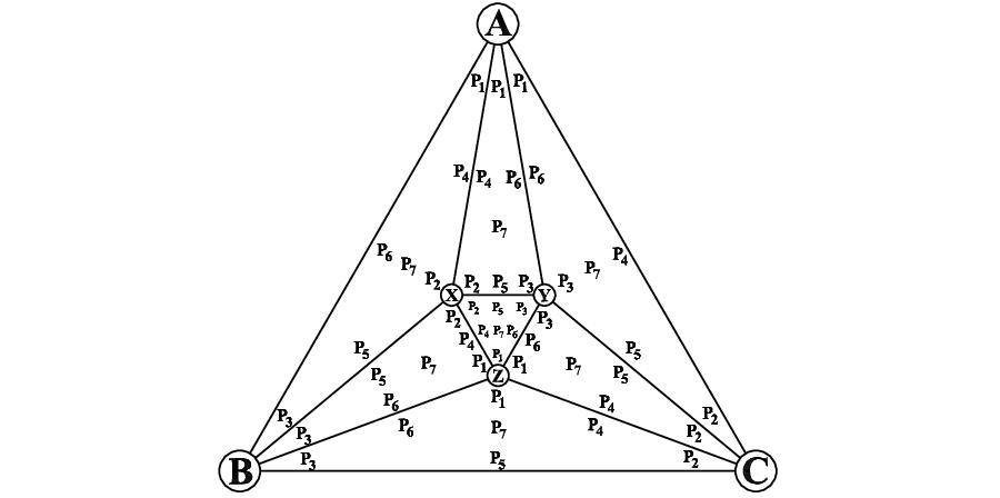
To calculate the crossing distance $\Delta_{t}^{1,2}$ , $\Delta_{t}^{1,3}$ , $\Delta_{t}^{1,4}$ , and $\sum_{j\in\Omega_{t}^{4}}d_{Aj}$ , we classify interior nodes in network $F_{t+1}$ into seven different parts according to their shortest path lengths to each of the three peripheral nodes (i.e. $A$ , $B$ , $C$ ). Notice that nodes $A$ , $B$ , $C$ themselves are not partitioned into any of the seven parts represented as $P_{1}$ , $P_{2}$ , $P_{3}$ , $P_{4}$ , $P_{5}$ , $P_{6}$ , and $P_{7}$ , respectively. The classification of nodes is shown in figure 6. For any interior node $v$ , we denote the shortest path lengths from $v$ to $A$ , $B$ , $C$ as $a$ , $b$ , and $c$ , respectively. By construction, $a$ , $b$ , $c$ can differ by at most $1$ since vertices $A$ , $B$ , $C$ are adjacent. Then the classification function $class(v)$ of node $v$ is defined to be

class(v)=\left\{\begin{array}[]{lc}{\displaystyle{P_{1}}}&\quad\hbox{for}\ a<b=c,\\ {\displaystyle{P_{2}}}&\quad\hbox{for}\ b<a=c,\\ {\displaystyle{P_{3}}}&\quad\hbox{for}\ c<a=b,\\ {\displaystyle{P_{4}}}&\quad\hbox{for}\ a=c<b,\\ {\displaystyle{P_{5}}}&\quad\hbox{for}\ a=b<c,\\ {\displaystyle{P_{6}}}&\quad\hbox{for}\ b=c<a,\\ {\displaystyle{P_{7}}}&\quad\hbox{for}\ a=b=c.\\ \end{array}\right.

(15)

It should be mentioned that the definition of node classification is recursive. For instance, class $P_{1}$ and $P_{4}$ in $F_{t}^{(1)}$ belong to class $P_{1}$ in $F_{t+1}$ , class $P_{3}$ and $P_{5}$ in $F_{t}^{(1)}$ belong to class $P_{2}$ in $F_{t+1}$ , class $P_{2}$ , $P_{6}$ , and $P_{7}$ in $F_{t}^{(1)}$ belong to class $P_{5}$ in $F_{t+1}$ . Since the three nodes $A$ , $B$ , and $C$ are symmetrical, in the network we have the following equivalent relations from the viewpoint of class cardinality: classes $P_{1}$ , $P_{2}$ , and $P_{3}$ are equivalent to one another, and it is the same with classes $P_{4}$ , $P_{5}$ , and $P_{6}$ . We denote the number of nodes in network $F_{t}$ that belong to class $P_{1}$ as $N_{t,P_{1}}$ , the number of nodes in class $P_{2}$ as $N_{t,P_{2}}$ , and so on. By symmetry, we have $N_{t,P_{1}}=N_{t,P_{2}}=N_{t,P_{3}}$ and $N_{t,P_{4}}=N_{t,P_{5}}=N_{t,P_{6}}$ . Therefore in the following computation we will only consider $N_{t,P_{1}}$ , $N_{t,P_{4}}$ , and $N_{t,P_{7}}$ . It is easy to conclude that

	$\displaystyle N_{t}$	$\displaystyle=N_{t,P_{1}}+N_{t,P_{2}}+N_{t,P_{3}}+N_{t,P_{4}}+N_{t,P_{5}}+N_{t,P_{6}}+N_{t,P_{7}}+3$
		$\displaystyle=3\,N_{t,P_{1}}+3\,N_{t,P_{4}}+N_{t,P_{7}}+3.$		(16)

Considering the self-similar structure of the network, we can easily know that at time $t+1$ , the quantities $N_{t+1,P_{1}}$ , $N_{t+1,P_{4}}$ , and $N_{t+1,P_{7}}$ evolve according to the following recursive equations

\displaystyle\left\{\begin{array}[]{ccc}N_{t+1,P_{1}}&=&3\,N_{t,P_{1}}+4\,N_{t,P_{4}}+N_{t,P_{7}}\,,\\ N_{t+1,P_{4}}&=&4\,N_{t,P_{1}}+N_{t,P_{4}}+N_{t,P_{7}}+1\,,\\ N_{t+1,P_{7}}&=&6\,N_{t,P_{4}}+N_{t,P_{7}}\,,\\ \end{array}\right.

where we have used the equivalent relations $N_{t,P_{1}}=N_{t,P_{2}}=N_{t,P_{3}}$ and $N_{t,P_{4}}=N_{t,P_{5}}=N_{t,P_{6}}$ . With the initial condition $N_{2,P_{1}}=4$ , $N_{2,P_{4}}=2$ , and $N_{2,P_{7}}=6$ , we can solve the recursive equation (III.3.3) to obtain

\displaystyle\left\{\begin{array}[]{ccc}N_{t,P_{1}}&=&\frac{1}{124}\left[-62+10\cdot 7^{t}+26\left(-1-\sqrt{2}\right)^{t}+26\left(-1+\sqrt{2}\right)^{t}+11\sqrt{2}\left(-1+\sqrt{2}\right)^{t}-11\sqrt{2}\left(-1-\sqrt{2}\right)^{t}\right]\,,\\ N_{t,P_{4}}&=&\frac{1}{124}\left[8\cdot 7^{t}-4\left(-1-\sqrt{2}\right)^{t}-4\left(-1+\sqrt{2}\right)^{t}+15\sqrt{2}\left(-1+\sqrt{2}\right)^{t}-15\sqrt{2}\left(-1-\sqrt{2}\right)^{t}\right],\\ N_{t,P_{7}}&=&\frac{1}{62}\left[62+4\cdot 7^{t}-33\left(-1-\sqrt{2}\right)^{t}-33\left(-1+\sqrt{2}\right)^{t}+39\sqrt{2}\left(-1-\sqrt{2}\right)^{t}-39\sqrt{2}\left(-1+\sqrt{2}\right)^{t}\right].\\ \end{array}\right.

For a node $v$ in network $F_{t+1}$ , we are also interested in the smallest value of the shortest path length from $v$ to any of the three peripheral nodes $A$ , $B$ , and $C$ . We denote the shortest distance as $f_{v}$ , which can be defined to be

f_{v}=min(a,b,c).

(25)

Let $d_{t,P_{1}}$ denote the sum of $f_{v}$ of all nodes belonging to class $P_{1}$ in network $F_{t}$ . Analogously, we can also define the quantities $d_{t,P_{2}}$ , $d_{t,P_{3}}$ , $\cdots$ , $d_{t,P_{7}}$ . Again by symmetry, we have $d_{t,P_{1}}=d_{t,P_{2}}=d_{t,P_{3}}$ , $d_{t,P_{4}}=d_{t,P_{5}}=d_{t,P_{6}}$ , and $d_{t,P_{1}}$ , $d_{t,P_{4}}$ , $d_{t,P_{7}}$ can be written recursively as follows:

\displaystyle\left\{\begin{array}[]{ccc}d_{t+1,P_{1}}&=&3\,d_{t,P_{1}}+4\,d_{t,P_{4}}+d_{t,P_{7}}\,,\\ d_{t+1,P_{4}}&=&4\,d_{t,P_{1}}+d_{t,P_{4}}+d_{t,P_{7}}+4\,N_{t,P_{1}}+1\,,\\ d_{t+1,P_{7}}&=&6\,(d_{t,P_{4}}+N_{t,P_{4}})+(d_{t,P_{7}}+N_{t,P_{7}})\,.\\ \end{array}\right.

Substituting equation (III.3.3) into equation (III.3.3), and considering the initial condition $d_{2,P_{1}}=4$ , $d_{2,P_{4}}=2$ , and $d_{2,P_{7}}=12$ , equation (III.3.3) is solved inductively

\displaystyle\left\{\begin{array}[]{ccc}d_{t,P_{1}}&=&\frac{1}{5004888}\Big[7\left(-3\left(-1+\sqrt{2}\right)^{t}\left(20082+18235\sqrt{2}\right)+\left(-1-\sqrt{2}\right)^{t}\left(-60246+54705\sqrt{2}\right)+4\left(29791+3327^{t}\right)\right)\\ &&+93\left(1760\times 7^{t}-7\left(-1+\sqrt{2}\right)^{t}\left(1256+1149\sqrt{2}\right)+\left(-1-\sqrt{2}\right)^{t}\left(-8792+8043\sqrt{2}\right)\right)t\Big],\\ d_{t,P_{4}}&=&\frac{1}{5004888}\Big[14\left(-59582+13700\times 7^{t}+\left(22941-56145\sqrt{2}\right)\left(-1-\sqrt{2}\right)^{t}+3\left(-1+\sqrt{2}\right)^{t}\left(7647+18715\sqrt{2}\right)\right)\\ &&+93\left(1408\times 7^{t}-7\left(-1+\sqrt{2}\right)^{t}\left(1042+107\sqrt{2}\right)+\left(-1-\sqrt{2}\right)^{t}\left(-7294+749\sqrt{2}\right)\right)t\Big],\\ d_{t,P_{7}}&=&\frac{1}{5004888}\Big[7\left(9\left(-1-\sqrt{2}\right)^{t}\left(-16540+33393\sqrt{2}\right)-9\left(-1+\sqrt{2}\right)^{t}\left(16540+33393\sqrt{2}\right)+8\left(29791+7424\times 7^{t}\right)\right)\\ &&+186\left(704\times 7^{t}-21\left(-1-\sqrt{2}\right)^{t}\left(-1149+628\sqrt{2}\right)+21\left(-1+\sqrt{2}\right)^{t}\left(1149+628\sqrt{2}\right)\right)t\Big].\end{array}\right.

III.3.4 Calculation of crossing distances

Having obtained the quantities $N_{t,P_{i}}$ and $d_{t,P_{i}}$ ( $i=1,2,\cdots,7$ ), we now begin to determine the crossing distance $\Delta_{t}^{1,2}$ , $\Delta_{t}^{1,3}$ , $\Delta_{t}^{1,4}$ , and $\sum_{j\in\Omega_{t}^{4}}d_{Aj}$ expressed as a function of $N_{t,P_{i}}$ and $d_{t,P_{i}}$ . Here we only give the computation details of $\Delta_{t}^{1,2}$ , while the computing processes of $\Delta_{t}^{1,3}$ , $\Delta_{t}^{1,4}$ , and $\sum_{j\in\Omega_{t}^{4}}d_{Aj}$ are similar. For convenience of computation, we use $\Gamma_{t}^{\eta,i}$ to denote the set of interior nodes belonging to class $P_{i}$ in $F_{t}^{(\eta)}$ . Then $\Delta_{t}^{1,2}$ can be written as

\Delta_{t}^{1,2}=\sum_{\stackrel{{\scriptstyle u\in\Gamma_{t}^{1,i},\,i\in\{1,2,3,4,5,6,7\}}}{{v\in F_{t}^{(2)},\,v\neq A,X,Y}}}d_{uv}.

(37)

The seven terms on the right-hand side of equation (37) are represented consecutively as $\delta_{t}^{i}$ ( $i=1,2,\cdots,7$ ). Next we will calculate the quantities $\delta_{t}^{i}$ . By symmetry, $\delta_{t}^{1}=\delta_{t}^{2}$ , $\delta_{t}^{5}=\delta_{t}^{6}$ . Therefore, we need only to compute $\delta_{t}^{1}$ , $\delta_{t}^{3}$ , $\delta_{t}^{4}$ , $\delta_{t}^{5}$ and $\delta_{t}^{7}$ . Firstly, we evaluate $\delta_{t}^{1}$ . By definition,

$\displaystyle\delta_{t}^{1}$	$\displaystyle=$	$\displaystyle\sum_{\stackrel{{\scriptstyle u\in\Gamma_{t}^{1,1},\,v\in F_{t}^{(2)}}}{{v\neq A,X,Y}}}d_{uv}$	(38)
	$\displaystyle=$	$\displaystyle\sum_{\stackrel{{\scriptstyle u\in\Gamma_{t}^{1,1},v\in\Gamma_{t}^{2,i}}}{{i\in\{1,4,6,7\}}}}(d_{uA}+d_{Av})+\sum_{\stackrel{{\scriptstyle u\in\Gamma_{t}^{1,1}}}{{v\in\Gamma_{t}^{2,3}}}}(d_{uA}+d_{AY}+d_{Yv})+\sum_{\stackrel{{\scriptstyle u\in\Gamma_{t}^{1,1}}}{{v\in\Gamma_{t}^{2,2}\bigcup\Gamma_{t}^{2,5}}}}(d_{uA}+d_{AX}+d_{Xv})$
	$\displaystyle=$	$\displaystyle N_{t,P_{1}}(3d_{t,P_{1}}+3d_{t,P_{4}}+d_{t,P_{7}}+2N_{t,P_{1}}+N_{t,P_{4}})+d_{t,P_{1}}(3N_{t,P_{1}}+3N_{t,P_{4}}+N_{t,P_{7}}).$

Proceeding similarly, we obtain

\displaystyle\delta_{t}^{3}=N_{t,P_{1}}(3d_{t,P_{1}}+3d_{t,P_{4}}+d_{t,P_{7}}+4N_{t,P_{1}}+3N_{t,P_{4}}+N_{t,P_{7}})+d_{t,P_{1}}(3N_{t,P_{1}}+3N_{t,P_{4}}+N_{t,P_{7}}),

(39)

\displaystyle\delta_{t}^{4}=N_{t,P_{2}}(3d_{t,P_{1}}+3d_{t,P_{4}}+d_{t,P_{7}}+N_{t,P_{1}})+d_{t,P_{2}}(3N_{t,P_{1}}+3N_{t,P_{4}}+N_{t,P_{7}}),

(40)

\displaystyle\delta_{t}^{5}=N_{t,P_{2}}(3d_{t,P_{1}}+3d_{t,P_{4}}+d_{t,P_{7}}+2N_{t,P_{1}}+N_{t,P_{4}})+d_{t,P_{2}}(3N_{t,P_{1}}+3N_{t,P_{4}}+N_{t,P_{7}}),

(41)

and

\displaystyle\delta_{t}^{7}=N_{t,P_{3}}(3d_{t,P_{1}}+3d_{t,P_{4}}+d_{t,P_{7}}+N_{t,P_{1}})+d_{t,P_{7}}(3N_{t,P_{1}}+3N_{t,P_{4}}+N_{t,P_{7}}).

(42)

With the obtained results for $\delta_{t}^{i}$ , we have

	$\displaystyle\Delta_{t}^{1,2}$	$\displaystyle=$	$\displaystyle 2(3d_{t,P_{1}}+3d_{t,P_{4}}+d_{t,P_{7}})(3N_{t,P_{1}}+3N_{t,P_{4}}+N_{t,P_{7}})+N_{t,P_{1}}(3N_{t,P_{1}}+3N_{t,P_{4}}+N_{t,P_{7}})$		(43)
			$\displaystyle+2(N_{t,P_{1}}+N_{t,P_{4}})(2N_{t,P_{1}}+N_{t,P_{4}})+N_{t,P_{1}}(N_{t,P_{4}}+N_{t,P_{7}})+(N_{t,P_{1}})^{2}.$		(43)

Analogously, we find

	$\displaystyle\Delta_{t}^{1,3}$	$\displaystyle=$	$\displaystyle 2(3d_{t,P_{1}}+3d_{t,P_{4}}+d_{t,P_{7}})(3N_{t,P_{1}}+3N_{t,P_{4}}+N_{t,P_{7}})+2(N_{t,P_{1}})^{2}+2N_{t,P_{1}}(3N_{t,P_{1}}+3N_{t,P_{4}}+N_{t,P_{7}})$		(44)
			$\displaystyle+N_{t,P_{4}}(3N_{t,P_{1}}+3N_{t,P_{4}}+N_{t,P_{7}})+(N_{t,P_{1}}+2N_{t,P_{4}}+N_{t,P_{7}})(2N_{t,P_{1}}+N_{t,P_{4}}),$		(44)

\displaystyle\Delta_{t}^{1,4}=2(3d_{t,P_{1}}+3d_{t,P_{4}}+d_{t,P_{7}})(3N_{t,P_{1}}+3N_{t,P_{4}}+N_{t,P_{7}})+(3N_{t,P_{1}}+3N_{t,P_{4}}+N_{t,P_{7}})^{2}+3(N_{t,P_{1}})^{2},

(45)

and

\sum_{j\in\Omega_{t}^{4}}d_{Aj}=(3d_{t,P_{1}}+3d_{t,P_{4}}+d_{t,P_{7}})+(3N_{t,P_{1}}+3N_{t,P_{4}}+N_{t,P_{7}})+N_{t,P_{1}}.

(46)

Substituting equations (43), (44), (45), and (46) into equation (14), we the final expression for cross distances $\Delta_{t}$ ,

$\displaystyle\Delta_{t}=\frac{1}{3844}$	$\displaystyle\Big[$	$\displaystyle 5766+2728\times 7^{t}+30290\times 49^{t}-10974\left(-1+\sqrt{2}\right)^{t}$	(47)
	$\displaystyle-$	$\displaystyle 9300\sqrt{2}\left(-1+\sqrt{2}\right)^{t}+3114\left(-1+\sqrt{2}\right)^{2t}$
	$\displaystyle+$	$\displaystyle 1017\sqrt{2}\left(-1+\sqrt{2}\right)^{2t}+186\left(-1-\sqrt{2}\right)^{t}\left(-59+50\sqrt{2}\right)$
	$\displaystyle-$	$\displaystyle 9\left(-1-\sqrt{2}\right)^{2t}\left(-346+113\sqrt{2}\right)+16368t\times 49^{t}\Big].$

III.3.5 Exact result for average path length

With the above-obtained results and recursion relations, we now readily calculate the sum of the shortest path lengths between all pairs of nodes. Inserting equation (47) into equation (12) and using the initial condition $D_{2}=717$ , equation (12) is solved inductively,

$\displaystyle D_{t}=\frac{1}{161448}$	$\displaystyle\bigg[$	$\displaystyle 201810+215270\times 7^{t}+11194\times 7^{2t}$	(48)
	$\displaystyle+$	$\displaystyle 72072\left(-1-\sqrt{2}\right)^{t}-57834\sqrt{2}\left(-1-\sqrt{2}\right)^{t}$
	$\displaystyle-$	$\displaystyle 44037\left(-1-\sqrt{2}\right)^{2t}-11340\sqrt{2}\left(-1-\sqrt{2}\right)^{2t}$
	$\displaystyle+$	$\displaystyle 72072\left(-1+\sqrt{2}\right)^{t}+57834\sqrt{2}\left(-1+\sqrt{2}\right)^{t}$
	$\displaystyle-$	$\displaystyle 44037\left(-1+\sqrt{2}\right)^{2t}+11340\sqrt{2}\left(-1+\sqrt{2}\right)^{2t}$
	$\displaystyle+$	$\displaystyle 16368t\times 7^{t}+16368t\times 7^{2t}\bigg].$

Substituting equation (48) into equation (10) yields the exactly analytic expression for average path length

$\displaystyle d_{t}=$		$\displaystyle\frac{1}{20181(15+8\times 7^{t}+7^{2t})}\bigg[201810$	(49)
	$\displaystyle+$	$\displaystyle 215270\times 7^{t}+11194\times 7^{2t}$
	$\displaystyle+$	$\displaystyle 72072\left(-1-\sqrt{2}\right)^{t}-57834\sqrt{2}\left(-1-\sqrt{2}\right)^{t}$
	$\displaystyle-$	$\displaystyle 44037\left(-1-\sqrt{2}\right)^{2t}-11340\sqrt{2}\left(-1-\sqrt{2}\right)^{2t}$
	$\displaystyle+$	$\displaystyle 72072\left(-1+\sqrt{2}\right)^{t}+57834\sqrt{2}\left(-1+\sqrt{2}\right)^{t}$
	$\displaystyle-$	$\displaystyle 44037\left(-1+\sqrt{2}\right)^{2t}+11340\sqrt{2}\left(-1+\sqrt{2}\right)^{2t}$
	$\displaystyle+$	$\displaystyle 16368t\times 7^{t}+16368t\times 7^{2t}\bigg].$

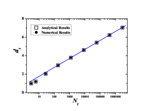
In the large $t$ limit, $d_{t}\sim t$ , while the network order $N_{t}\sim 7^{t}$ which is obvious from equation (1). Thus, the average path length grows logarithmically with increasing order of the network. We have checked our analytic result provided by equation (49) against numerical calculations for different network order up to $t=8$ which corresponds to $N_{8}=1\,007\,772$ . In all the cases we obtain a complete agreement between our theoretical formula and the results of numerical investigation, see figure 7.

Recently, it has been suggested that for random uncorrelated scale-free networks (SFNs) with degree exponent $\gamma<3$ and network order $N$ , their average distance $d(N)$ behaves as a double logarithmic scaling with $N$ : $d(N)\sim\ln\ln N$ [53, 52]. However, for the deterministic network considered here, in despite of the fact that its degree exponent $\gamma=1+\frac{\ln 7}{\ln 3}<3$ , its average path length scales as a logarithmic scaling with network order, showing a obvious difference from that of the stochastic scale-free counterparts. The logarithmic scaling of $d_{t}$ with $N_{t}$ for our network as well as the Apollonian networks [41] shows that previous relation between APL and the network order obtained for uncorrelated SFNs [53, 52] is not valid for disassortative SFNs [53, 52], at least for some spatial networks, e.g., the Apollonian networks and the network considered here. This leads us to the conclusion that degree exponent itself does not suffice to characterize the APL of SFNs.

III.4 Degree correlations

An interesting quantity related to degree correlations is the average degree of the nearest neighbors for nodes with degree $k$ , denoted as $k_{\rm nn}(k)$ , which is a function of node degree $k$ [54, 55]. When $k_{\rm nn}(k)$ increases with $k$ , it means that nodes have a tendency to connect to nodes with a similar or larger degree. In this case the network is defined as assortative [5]. In contrast, if $k_{\rm nn}(k)$ is decreasing with $k$ , which implies that nodes of large degree are likely to have near neighbors with small degree, then the network is said to be disassortative. If correlations are absent, $k_{\rm nn}(k)=const$ .

We can exactly calculate $k_{\rm nn}(k)$ for network $F_{t}$ using equations (3) and (4) to work out how many links are made at a particular step to nodes with a particular degree. By construction, we have the following expression [56, 57]

	$\displaystyle k_{\rm nn}(k)$	$\displaystyle=$	$\displaystyle{1\over L_{v}(t_{i})k(t_{i},t)}\Bigg[\sum_{t^{\prime}_{i}=0}^{t^{\prime}_{i}=t_{i}-1}2L_{v}(t^{\prime}_{i})L_{\Delta}(t^{\prime}_{i},t_{i}-1)k(t^{\prime}_{i},t)$		(50)
			$\displaystyle+\sum_{t^{\prime}_{i}=t_{i}+1}^{t^{\prime}_{i}=t}2L_{v}(t_{i})L_{\Delta}(t_{i},t^{\prime}_{i}-1)k(t^{\prime}_{i},t)\Bigg]+2$		(50)

for $k=4\times 3^{t-t_{i}}$ ( $t_{i}\geq 1$ ), where $k(t_{i},t)$ is the degree of a node $i$ at time $t$ that was born at step $t_{i}$ . Here the first sum on the right-hand side accounts for the links made to nodes with larger degree (i.e. $t^{\prime}_{i}<t_{i}$ ) when the node was generated at $t_{i}$ . The second sum describes the links made to the current smallest degree nodes at each step $t^{\prime}_{i}>t_{i}$ . The last term 2 accounts for the two links connected to two simultaneously emerging nodes. After some algebraic manipulations, we can rewrite equation (50) in term of $k$ to obtain

\displaystyle k_{\rm nn}(k)=\frac{(3^{2\,t+1}+3^{t-1})\left(\frac{4}{k}\right)^{2-\ln 7/\ln 3}}{2\times 7^{t-1}}+\frac{8\ln(\frac{k}{4})}{3\ln 3}-10.

(51)

For $k=3^{t}+1$ ( $t_{i}=0$ ), we have

	$\displaystyle k_{\rm nn}(k)$	$\displaystyle=$	$\displaystyle{1\over k(t_{i},t)}\Bigg[\sum_{t^{\prime}_{i}=t_{i}+1}^{t^{\prime}_{i}=t}2L_{\Delta}(t_{i},t^{\prime}_{i}-1)k(t^{\prime}_{i},t)\Bigg]+2$		(52)
		$\displaystyle=$	$\displaystyle\frac{8t\times 3^{t}}{3^{t+1}+3}+2.$		(52)

Therefore, for large $t$ and $k$ , $k_{\rm nn}(k)$ is approximately a power law function of $k$ as $k_{\rm nn}(k)\sim k^{-\omega}$ with $\omega=2-\frac{\ln 7}{\ln 3}\simeq 0.229$ , which shows that the network is disassortative. Note that $k_{\rm nn}(k)$ of the Internet exhibits a similar power-law scaling with exponent $\omega=0.5$ [54].

IV Conclusion

In summary, motivated by the disk packing and Apollonian networks, we have presented a model for spatial planar networks introducing the influence of geography encoded in the disk packing. According to the construction, we have studied analytically the main structural features of the network. We have shown that the network has a power law distribution with exponent $\gamma=1+\frac{\ln 7}{\ln 3}$ , it has a large clustering coefficient 0.603, its APL scales logarithmically with the number of network nodes, and it is disassortative with the average degree of the nearest neighbors for nodes having degree $k$ being roughly a power-law function of $k$ with exponent -0.229.

Note that although both the network considered here and the Apollonian network [38, 56] are translated from disk packings, and both networks have qualitatively similar topologies, their structural characteristics are quantitatively different. For example, the exponent of degree distribution is $1+\frac{\ln 7}{\ln 3}$ for our network, while for Apollonian network it is $1+\frac{\ln 3}{\ln 2}$ ; the average clustering coefficients for our network and Apollonian network are 0.603 and 0.828, respectively. In addition, the average path length [41] and the degree correlations [56] for both networks are also of quantitative difference. These disparities of the two networks show that the ways of disk packing lead to different spatial constrains of network nodes, which in turn have a significant impact on network properties and thus dynamics running on networks, such as cascading failing [25], random walks [58], and so on. Thus, we can conclude that for spatial networks the positions, where nodes are geographically located, matter greatly and should be incorporated when modeling such networks. Ignoring the geography will lead to miss some important attributes and properties of the systems.

Acknowledgment

We would like to thank Yichao Zhang and Ming Yin for their help. This research was supported by the National Basic Research Program of China under grant No. 2007CB310806, the National Natural Science Foundation of China under Grant Nos. 60704044, 60873040 and 60873070, Shanghai Leading Academic Discipline Project No. B114, and the Program for New Century Excellent Talents in University of China (NCET-06-0376).

References

[1] R. Albert and A.-L. Barabási, Rev. Mod. Phys. 74, 47 (2002).
[2] S. N. Dorogovtsev and J.F.F. Mendes, Adv. Phys. 51, 1079 (2002).
[3] A.-L. Barabási and R. Albert, Science 286, 509 (1999).
[4] D.J. Watts and H. Strogatz, Nature (London) 393, 440 (1998).
[5] M. E. J. Newman, Phys. Rev. Lett. 89, 208701 (2002).
[6] M. E. J. Newman, SIAM Review 45, 167 (2003).
[7] S. Boccaletti, V. Latora, Y. Moreno, M. Chavez, and D.-U. Hwanga, Phy. Rep. 424, 175 (2006).
[8] S. N. Dorogovtsev, A. V. Goltsev and J.F.F. Mendes, Rev. Mod. Phys. 80, 1275 (2008).
[9] S.N. Dorogovtsev, J.F.F. Mendes, A.N. Samukhin, Phys. Rev. Lett. 85, 4633 (2000).
[10] L.A.N. Amaral, A. Scala, M. Barthélémy, H.E. Stanley, Proc. Natl. Acad. Sci. U.S.A. 97, 11149 (2000).
[11] G. Bianconi, A.-L. Barabási, Europhys. Lett. 54, 436 (2001).
[12] F. Chung, L.Y. Lu, T.G. Dewey, D.J. Galas, Biology 10, 677 (2003).
[13] A. Barrat, M. Barthélemy, and A. Vespignani, Phys. Rev. Lett. 92, 228701 (2004).
[14] W.-X. Wang, B.-H. Wang, B. Hu, G. Yan, Q. Ou, Phys. Rev. Lett. 94, 188702 (2005).
[15] J. S. Mattick and M. J. Gagen, Science 307, 856 (2005).
[16] Z. Z. Zhang, L. J. Fang, S. G. Zhou, and J. H. Guan, Physica A 388, 225 (2009).
[17] T. Gross and B. Blasius, J. R. Soc. Interface 5, 259 (2008).
[18] L. Lacasa, B. Luque, F. Ballesteros, J. Luque, and J. C. Nuño, Proc. Natl. Acad. Sci. U.S.A. 105, 4972 (2008).
[19] M. E. J. Newman, Proc. Natl. Acad. Sci. U.S.A. 98, 404 (2001).
[20] H. Jeong, B. Tombor, R. Albert, Z. N. Oltvai and A.-L. Barabási, Nature 407, 651 (2000).
[21] M. Faloutsos, P. Faloutsos and C. Faloutsos, Comput. Commun. Rev. 29, 251 (1999).
[22] R. Albert, I. Albert, and G. L. Nakarado, Phys. Rev. E 69, 025103(R) (2004).
[23] A. Barrat, M. Barthélemy, R. Pastor-Satorras, and A. Vespignani, Proc. Natl. Acad. Sci. U.S.A. 101, 3747 (2004).
[24] Y. Hayashi and J. Matsukubo, Phys. Rev. E 73, 066113 (2006).
[25] L. Huang, L. Yang, and K. Yang, Phys. Rev. E 73, 036102 (2006).
[26] C.-Y. Yin, B.-H. Wang, W.-X. Wang and G. R. Chen, Phys. Rev. E 77, 027102 (2008).
[27] C. P. Warren, L. M. Sander, and I. M. Sokolov, Phys. Rev. E 66, 056105 (2002).
[28] A. Cardillo, S. Scellato, V. Latora, and S. Porta, Phys. Rev. E 73, 066107 (2006).
[29] R. Ferrer-i-Cancho, C. Janssen, and R. V. Solé, Phys. Rev. E 64, 046119 (2001).
[30] J. Buhl, J. Gautrais, J. Louis Deneubourg, P. Kuntz, and G. Theraulaz, J. Theor. Biol. 243, 287 (2006).
[31] O. Sporns, Complexity 8, 56 (2003).
[32] A. F. Rozenfeld, R. Cohen, D. ben-Avraham, and S. Havlin, Phys. Rev. Lett. 89, 218701 (2002).
[33] S. S. Manna and P. Sen, Phys. Rev. E 66, 066114 (2002).
[34] M. Barthélemy, Europhys. Lett. 63, 915 (2003).
[35] N. Masuda, H. Miwa, and N. Konno, Phys. Rev. E 71, 036108 (2005).
[36] M. T. Gastner and M. E. J. Newman, Eur. Phys. J. B 49, 247 (2006).
[37] K. Kosmidis, S. Havlin, and A. Bunde, EPL 82, 48005 (2008).
[38] J.S. Andrade Jr., H.J. Herrmann, R.F.S. Andrade and L.R.da Silva, Phys. Rev. Lett. 94, 018702 (2005).
[39] Z.Z. Zhang, F. Comellas, G. Fertin and L.L. Rong, J. Phys. A: Math. Gen. 39, 1811 (2006).
[40] Z. Z. Zhang, L. L. Rong, and S. G. Zhou, Phys. Rev. E, 74, 046105 (2006).
[41] Z. Z. Zhang, L. C. Chen, S. G. Zhou, L. J. Fang, J. H. Guan, and T. Zou, Phys. Rev. E 77, 017102 (2008).
[42] A. P. Vieira, J. S. Andrade, Jr., H. J. Herrmann, and R. F. S. Andrade, Phys. Rev. E 76, 026111 (2007).
[43] I. N. de Oliveira, F. A. B. F. de Moura, M. L. Lyra, J. S. Andrade, Jr., and E. L. Albuquerque, Phys. Rev. E 79, 016104 (2009).
[44] H. J. Herrmann, G. Mantica and D. Bessis, Phys. Rev. Lett. 65, 3223 (1990).
[45] S. S. Manna and H.J. Herrmann, J. Phys. A: Math. Gen. 24, L481 (1991).
[46] D. W. Boyd, Canadian Journal of Mathematics 25, 303 (1973).
[47] D.B. West, Introduction to Graph Theory (Prentice-Hall, Upper Saddle River, NJ, 2001).
[48] E. Ravasz and A.-L. Barabási, Phys. Rev. E 67, 026112 (2003).
[49] M. Hinczewski and A. N. Berker, Phys. Rev. E 73, 066126 (2006).
[50] Z. Z. Zhang, S. G. Zhou, and T. Zou, Eur. Phys. J. B 58, 337 (2007).
[51] Z. Z. Zhang, S. G. Zhou, Z. Y. Wang, and Z. Shen, J. Phys. A: Math. Theor. 40, 11863 (2007).
[52] F. Chung and L. Lu, Proc. Natl. Acad. Sci. U.S.A. 99, 15879 (2002).
[53] R. Cohen and S. Havlin, Phys. Rev. Lett. 90, 058701 (2003).
[54] R. Pastor-Satorras, A. Vázquez and A. Vespignani, Phys. Rev. Lett. 87, 258701 (2001).
[55] A. Vázquez, R. Pastor-Satorras and A. Vespignani, Phys. Rev. E 65, 066130 (2002).
[56] J. P. K. Doye and C. P. Massen, Phys. Rev. E 71, 016128 (2005).
[57] Z. Z. Zhang, L. L. Rong, S. G. Zhou, Physica A 377, 329 (2007).
[58] Z. Z. Zhang, J. H. Guan, W. L. Xie, Y. Qi, and S. G. Zhou, EPL 86, 10006 (2009).