e-mail jernej.mravlje@ijs.si
XXXX
[height=3.1cm,keepaspectratio]Fig1.eps \titlefigurecaptionSketch of the model device. The overlap integrals between the molecular orbital and the leads ( for left, right lead, respectively) are modulated by the position of the molecule. The energy of the molecular level is determined by the gate voltage.
Kondo effect in oscillating molecules
Abstract
\abstcolWe consider electronic transport through break-junctions bridged by a single molecule in the Kondo regime. We describe the system by a two-channel Anderson model. We take the tunneling matrix elements to depend on the position of the molecule. It is shown, that if the modulation of the tunneling by displacement is large, the potential confining the molecule to the central position between the leads is softened and the position of the molecule is increasingly susceptible to external perturbations that break the inversion symmetry. In this regime, the molecule is attracted to one of the leads and as a consequence the conductance is small. We argue on semi-classical grounds why the softening occurs and corroborate our findings by numerical examples obtained by Wilson’s numerical renormalization group and Schönhammer-Gunnarsson’s variational method.
pacs
72.15.Qm,73.23.-b,73.22.-f1 Introduction and model
In recent years considerable advance has been achieved in manufacturing mesoscopic systems, which due to their tunability with external electrodes provide a playground for research in the correlated electron systems. For example, the Kondo effect – generic name for phenomena related to increased scattering off impurities with internal degrees of freedom – was observed in measurements of electron transport through quantum dots [1], atoms, and molecules [2, 3, 4, 5, 6, 7, 8].
Unlike in experiments with quantum dots, the transport through break junctions is strongly affected by the molecular vibrational modes, because the frequency of the oscillations is of comparable magnitude than other energy scales, such as Coulomb repulsion. For example, the side-peaks in the non-linear conductance [4, 5, 6] were observed indicating the transfer of energy from the oscillations to the electron current. By comparing the observed frequencies to the frequencies of the molecular internal modes it was shown [4], that in some cases also the oscillations of the molecule with respect to the leads have to be taken into account.
In this work we concentrate on such a case. The tunneling is generally dependent on the overlap between the wave-functions. This motivates us to investigate the effects of the modulation of the tunneling matrix elements by molecular oscillations.
More specifically, we describe the break junction by a model consisting of two metallic leads (half-filled bands of non-interacting electrons). The leads are bridged by a single molecule which we assume is confined harmonically to the center between the leads. The position of the molecule determines the tunneling matrix elements. Assuming the leads are identical and the displacement of the molecule from the center of inversion is small [9], the tunneling matrix elements towards left and right leads read .
The Hamiltonian consists of several parts
| (1) |
The first two terms describe the isolated leads
| (2) |
is the lead index, is the spin index and the wave-vector index; (as well as to be introduced below) denote the fermion creation operators. The precise form of the band dispersion is not important for the results presented here, provided the density of states is smooth and symmetric around the Fermi surface; nevertheless for definiteness we note that in our calculations we used flat (NRG simulations) and tight-binding bands (simulations with Schönhammer-Gunnarsson wave functions).
The second term describes the molecular orbital (we assume a single molecular level participates actively in the transport),
| (3) |
where counts the number of electrons occupying the orbital, the energy of the orbital relative to the chemical potential of the leads, is the Coulomb repulsion. We concentrate on the particle-hole symmetric case . describes the phonon mode ( is the phonon creation operator).
The coupling between the leads, the molecular orbital and also phonons is described by
| (4) | |||||
Here we introduced a constant , which we will use to test for the influence of the breaking of the inversion symmetry; for the Hamiltonian is symmetric with respect to operation ; finite breaks this symmetry.
In the model with no coupling to phonons () for only the even combination of the operators, i.e. (other indeces are suppressed) in the leads is coupled to the molecular orbital. The life time of electrons on the orbital is finite due to the tunneling to the leads; the hybridization (inverse life-time) for the flat band reads , where is the density of states in each of the two leads (for flat band of half-width , . The odd linear combinations are decoupled. For and still a particular linear combination of the states in the leads is decoupled and the system can be described by the single-channel model.
For finite this no longer holds and the molecule is coupled to both conduction channels. Rewriting the coupling term in the even-odd basis,
| (5) |
makes it manifest that we are dealing with a two-channel Anderson model. No linear combination of the conduction electrons can be integrated out because the coupling to the odd channel is mediated by phonons. This occurs because the modulation of tunneling is antisymmetric with respect to inversion; if the modulation of tunneling is symmetric [10, 11] the orbital is still coupled only to the even channel.
It is difficult to access the low temperature (Kondo) regime because of the presence of exponentially small energy scale ( is the magnitude of the exchange coupling). Only few methods [12] reproduce the increase of conductance towards the unitary limit for temperatures smaller than accurately. On the other hand, in the high-temperature regime (relevant for nanoelectromechanical systems [13, 14, 15]) it is adequate to ignore the Kondo correlations and take only lowest orders in tunneling into account.
For the work on this model in the Kondo regime, which was originally stimulated by Ref. [16], we refer the reader to Refs. [17, 18, 19, 9]. Another very recent paper discusses a similar model as an example of two-level system [20].
In the following section we first demonstrate that the confining potential is weakened by the electron-phonon coupling and can even be driven to a form of the double-well. Then we give numerical examples on how the emergence of the double-well potential affects static and dynamic properties of the molecule. Finally, we show that when the inversion symmetry is not perfect (), the electron-phonon coupling will drive the molecule away from the central position. As a consequence, in this regime the conductance can be significantly suppressed.
2 The emergence of a double well potential
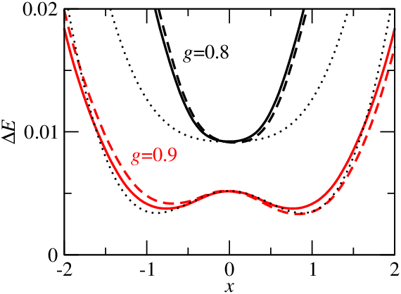
It is easy to demonstrate that a double well effective oscillator potential may form under the influence of a sufficient electron-phonon coupling , where we define the delimiting value of the coupling constant. For we can make a simple estimate on the form of the effective oscillator potential by a substitution , where is a real-valued constant. In the wide-band limit ( small) the energy gain due to the hybridization is [21] , where we use the effective displacement-dependent hybridization . The elastic energy cost is , hence in this semi-classical approximation the dependence of energy on can be written in a closed form
| (6) |
The prefactor of the -term in the small- expansion is equal to , hence for increasing the elastic potential is softened and a double well effective potential emerges for
| (7) |
We plot for and in Fig. 1 (thin, dotted lines).
We estimate the effective potential also numerically using a variational method based on the Schönhammer-Gunnarsson [22, 23] wave fuction (the details of our implementation are given in our previous work [24, 25, 11]). Briefly, the idea is to find an auxiliary non-interacting Hamiltonian [of the same form as in Eq. (1), but for and renormalized parameters ], which minimizes the variational ground state energy . The variational function is expressed in the basis of projection operators acting on the Hartree-Fock ground state (which includes the phonon vacuum) of the auxiliary Hamiltonian ,
| (8) |
To obtain the ground state, we minimize energy with respect to all the parameters of . On the other hand, by restricting the minimization to a particular subspace (for example, by fixing the ratio ) we obtain the variational wave-function for which the expectation value is a function of . The pairs constitute our estimate of the effective potential and are plotted in Fig. 1 for (full lines) and (dashed lines). The agreement between the semi-classical estimate and numerical results is reasonable.
The perturbation breaks the inversion symmetry, therefore the right minima in regime in this case is lower in energy. In this regime, the molecule will predominantly reside near the right lead. Conversely, for the potential is only slightly perturbed.
3 NRG results
Having established well the emergence of the double well effective potential we now check how it is reflected first in the static properties and then the dynamical response of the system. To obtain these quantities, we have performed the numerical simulations using the well known Wilson’s numerical renormalization group [26, 27](NRG) method. We restrict ourselves to the limit of zero temperature (). The details of the calculations are given in Ref. [9].

3.1 Static quantities
We begin by looking at the static quantities. The average displacement for vanishes (as expected for an operator of odd parity under inversion in a state of well-defined parity). The fluctuations of displacement , shown in Fig. 2 (full line) increase monotonically with . The slope of is increased considerably at [or , see Ref. [9]], where the double well like effective potential is formed. This change of slope is driven by the increased hybridization in the odd-channel.
For the absence of inversion symmetry is reflected in the nonvanishing average displacement (dashed-dotted), which monotonically increases with increasing . Therefore the fluctuations of displacement (dashed) in this case reach a maximum and then decrease with increasing .
For comparison, we plot also the position of the minimum of the potential (dotted line) obtained from the semi-classical estimate Eq. (6),
| (9) |
3.2 Phonon propagator

Now we turn to the renormalization of the phonon propagator by the electron-phonon coupling. The dynamical information about oscillator is contained in the displacement Green’s function. The displacement spectral function
| (10) |
is an odd function of due to the hermiticity of . Since is in NRG evaluated for a finite system it consists of several -peaks of different weights. To obtain a smooth spectral function we have used the Gaussian broadening on the logarithmic scale [28], where the Dirac function is broadened according to
| (11) |
and we used in our calculations.
In Fig. 3 we plot for various and . The width of the high frequency peaks is overestimated due to the broadening procedure described above (for example, the width of the peak at for should vanish). We could use the Dyson equation [29, 30] to obtain sharper peaks but we avoid this complication because on one hand there is no a priori guarantee that such a procedure gives more accurate results for large and on the other hand in this work we are interested only in the position and not the width of the peaks.
For intermediate (starting at for the parameters used here) the vibrational mode begins to soften; the characteristic frequency of the oscillations is decreased. At still larger two peaks emerge. The high frequency peak corresponds to the oscillations within each of the minima of the double-well potential, and the low-frequency peak (we denote its position by ) corresponds to the slow tunneling between the degenerate (or near-degenerate for ) minima.
The propagators for finite and look alike, provided is small enough that does not decrease below the frequency given by the energy difference between the minima of the two wells.
For larger the high frequency behaviour remains similar but as shown in Fig. 4 which decreases for exponentially (full line), for finite (dashed) saturates to the value of the energy difference between the minima. In this regime, the tunneling of the oscillator between the minima as characterized by the weight of the soft-mode peak in the phonon propagator (shown dotted) is suppressed.

3.3 Conductance

We show the conductance calculated by NRG in Fig. 5. In the particle-hole symmetric point and at zero temperature the system is in the unitary limit, hence the conductance (in units of ) is for near unity (reduced only due to small breaking of inversion symmetry for a value of order ). For increasing it decreases and at if drops to zero. This occurs because the molecular orbital is increasingly hybridized only to the right lead and the coupling to left lead becomes small. The point where the conductance is zero corresponds to the decoupling of the left lead, , on the average.
Surprisingly, for larger still, the conductance increases again. This is due to the overlap with the negative amplitude when states for which contribute considerably to the transport. As discussed in more detail in Ref. [9] this regime is an artifact of linearization and cannot be observed in the break-junction experiments. Here we remark only, that in the large- regime the spin is screened by the odd channel. At the delimiting value of (which we denote by ) the spin is simultaneously screened by the both channels and the resulting state is characterized by the non-Fermi liquid two-channel Kondo fixed point in the NRG flow.
4 Conclusions
In this report we considered a metallic break-junction bridged by a molecule. We were interested in the electron transport through the break-junction, which is influenced by the modulation of tunneling between the molecular orbital and the leads due to the oscillations of the molecule with respect to the leads.
We have shown that due to the electron-phonon coupling the harmonic potential confining the molecule to the center-of-inversion evolves to the double well effective potential. The change in the form of confining potential is reflected in dynamical properties – e.g. a low-frequency peak emerges in the phonon propagator – as well as in the static properties – e.g. the fluctuations of displacement are increased.
The emergence of the double well effective potential makes the system strongly susceptible to perturbations breaking the inversion symmetry. When the frequency of the soft-mode decreases below the energy scale of such a perturbation, the molecule is attracted to one of the leads. As a consequence, the conductance is suppressed.
There are many points which we have not discussed in detail, including the breakdown of the linearization and the physics of the two-channel Kondo fixed point. The more comprehensive analysis of this interesting system will appear elsewhere [9].
We acknowledge the use of R. Žitko’s NRG http://nrgljubljana.ijs.si and T. Rejec’s SG code.
References
- [1] D. Goldhaber-Gordon, H. Shtrikman, D. Mahalu, D. Abusch-Magder, U. Meirav, and M. A. Kastner, Nature 391, 156 (1998).
- [2] V. Madhavan, W. Chen, T. Jamneala, M. F. Crommie, and N. S. Wingreen, Science 280, 567 (1998).
- [3] W. Liang, M. P. Shores, M. Bockrath, J. R. Long, and H. Park, Nature 417, 725 (2002).
- [4] J. Park, A. N. Pasupathy, J. I.Goldsmith, C. Chang, Y. Yaish, J. R. Petta, M. Rinkoski, J. P. Sethna, H. D. Abrunas, P. L. McEuen, and D. C. Ralph, Nature 417, 722 (2002).
- [5] L. H. Yu and D. Natelson, Nano Lett. 4, 79 (2005).
- [6] A. N. Pasupathy, J. Park, C. Chang, A. V. Soldatov, S. Lebedkin, R. C. Bialczak, J. E. Grose, L. A. K. Donev, J. P. Sethna, D. C. Ralph, and P. L. McEuen, Nano Lett. 5, 203 (2005).
- [7] A. Zhao, Q. Li, L. Chen, H. Xiang, W. Wang, S. Pan, B. Wang, X. Xiao, J. Yang, J. G. Hou, and Q. Zhu, Science 309(5740), 1542 (2005).
- [8] L. H. Yu, Z. K. Keane, J. W. Ciszek, L. Cheng, J. M. Tour, T. Baruah, M. R. Pederson, and D. Natelson, Phys. Rev. Lett. 95, 256803 (2005).
- [9] In J. Mravlje and A. Ramšak, Phys. Rev. B. 78, 235416 (2008) a more general case of modulation is considered.
- [10] P. S. Cornaglia, D. R. Grempel, and H. Ness, Phys. Rev. B 71(7), 075320 (2005).
- [11] J. Mravlje, A. Ramšak, and T. Rejec, Phys. Rev. B 72, 121403(R) (2005).
- [12] J. Bonča, A. Ramšak, and T. Rejec, unpublished (2004), arXiv:cond-mat/0407590.
- [13] T. Novotný, A. Donarini, C. Flindt, and A. P. Jauho, Phys. Rev. Lett. 92(24), 248302 (2004).
- [14] J. Twamley, D. W. Utami, H. S. Goan, and G. Milburn, New J. Phys. 8(5), 63 (2006).
- [15] J. R. Johansson, L. G. Mourokh, A. Y. Smirnov, and F. Nori, Phys. Rev. B 77(3), 035428 (2008).
- [16] K. A. Al-Hassanieh, C. A. Büsser, G. Martins, and E. Dagotto, Phys. Rev. Lett. 95, 256807 (2005).
- [17] C. A. Balseiro, P. S. Cornaglia, and D. R. Grempel, Phys. Rev. B 74(23), 235409 (2006).
- [18] J. Mravlje, A. Ramšak, and T. Rejec, Phys. Rev. B 74(20), 205320 (2006).
- [19] J. Mravlje, A. Ramšak, and R. Žitko, Physica B 403, 1484 (2008).
- [20] P. Lucignano, G. E. Santoro, M. Fabrizio, and E. Tosatti, Phys. Rev. B 78, 155418 (2008).
- [21] M. Fabrizio, Lectures on the physics of strongly correlated systems, (AIP, 2007), chap. I, edited by A. Avella and F. Mancini, p. 3.
- [22] K. Schönhammer, Phys. Rev. B 13(10), 4336 (1976).
- [23] O. Gunnarsson and K. Schönhammer, Phys. Rev. B 31(8), 4815 (1985).
- [24] T. Rejec and A. Ramšak, Phys. Rev. B 68, 033306 (2003).
- [25] T. Rejec and A. Ramšak, Phys. Rev. B 68(3), 035342 (2003).
- [26] K. G. Wilson, Rev. Mod. Phys. 47, 773 (1975).
- [27] R. Bulla, T. A. Costi, and T. Pruschke, Rev. Mod. Phys. 80(2), 395 (2008).
- [28] R. Bulla, T. A. Costi, and D. Vollhardt, Phys. Rev. B 64(4), 045103 (2001).
- [29] A. C. Hewson, R Bulla, and T. Pruschke, J. Phys: Condens. Matter 10(37), 8365 (1998).
- [30] G. S. Jeon, T. H. Park, and H. Y. Choi, Phys. Rev. B 68(4), 045106 (2003).