Relaxation of Josephson qubits due to strong coupling to two-level systems

First, we consider the simplest case, in which only the TLF is coupled to a dissipative bath and this coupling is transverse. The coupling operator in Eq. (2) takes the form

where the bath variable $\hat{X}_{f,\perp}$ is characterized by the (non-symmetrized) correlation function $C_{f,\perp}(t)\equiv\left\langle\hat{X}_{f,\perp}(t)\hat{X}_{f,\perp}(0)\right\rangle$. In thermal equilibrium we have $C_{f,\perp}(-\omega)=e^{-\omega/T}C_{f,\perp}(\omega)$. We assume here that $T\ll\epsilon_{f}$, i.e., that the temperature is effectively zero, so that we can neglect excitations.

We solve the Bloch-Redfield equations [28, 29] for the coupled system using the secular approximation. As the initial condition we take the qubit in the excited state and the TLF in its thermal equilibrium state. Tracing out the TLF’s degrees of freedom we find the dynamics of $\left\langle\sigma_{z}\right\rangle$ (Fig. 2).

For the expectation value $\left\langle\sigma_{z}\right\rangle$ we find the following expression

where $\left\langle\sigma_{z}\right\rangle_{\infty}\approx-1$ is the zero-temperature equilibrium value. We can separate the right-hand side of Eq. (4) into damped oscillations, with decay rate $\Gamma_{osc}$, and a purely decaying part. The amplitude and the decay rate of the oscillating part are given by

Here the rate

is the relaxation rate of the fluctuator. We observe that the decay rate of the oscillations, $\Gamma_{osc}$, is independent of the coupling strength $v_{\perp}$ and of the detuning $\delta\omega$. Note that the physics considered here is only relevant near the resonance $\epsilon_{f}\approx\epsilon_{q}$, and we assume that the spectrum $C_{f,\perp}(\omega)$ is sufficiently smooth in this region, so that $C_{f,\perp}(\epsilon_{f})\approx C_{f,\perp}(\epsilon_{q})$.

For the purely decaying part we find

where $\Gamma_{10}^{f}$ and $\Gamma_{20}^{f}$ are the rates with which the states $\left|1\right\rangle$ and $\left|2\right\rangle$ decay into the ground state $\left|0\right\rangle$ (cf. Fig. 3).

As we can see, the decay law for $\left\langle\sigma_{z}(t)\right\rangle-\left\langle\sigma_{z}\right\rangle_{\infty}$ is given by a sum of several exponents. It is sometimes useful, e.g., for comparison with experiments where no fitting to a specific decay law was performed, to define a single decay rate for the whole process. If a function $f(t)$ decays from $f(t=0)=a$ to $f(t\rightarrow\infty)=0$, we can define the single decay rate $\Gamma$ from $\int_{0}^{\infty}f(t)dt=a/\Gamma$.

We can introduce the single decay rate in two different ways, either effectively averaging over the oscillations or including all parts and describing the envelope curve (cf. Fig. 2). In the first case, averaging over the oscillations, we choose $f(t)=a_{\downarrow,1}\>e^{-\Gamma_{\downarrow,1}\>t}+a_{\downarrow,2}\>e^{-\Gamma_{\downarrow,2}\>t}$ and obtain for the amplitude and the decay rate

This gives a quasi-Lorentzian line shape of $\Gamma_{av}(\delta\omega)$ with the width of the order of the coupling $v_{\perp}$ and the maximum value at resonance of $\Gamma_{av}(\delta\omega=0)=\frac{1}{2}\>\gamma_{1}^{f}$.

Figure 4 shows the amplitudes and rates characterizing the decay of the oscillations (dashed red) and of the purely decaying part (solid blue) of the qubits $\left\langle\sigma_{z}\right\rangle$.

To describe the envelope we choose $f(t)=a_{\downarrow,1}\>e^{-\Gamma_{\downarrow,1}\>t}+a_{\downarrow,2}\>e^{-\Gamma_{\downarrow,2}\>t}+a_{osc}\>e^{-\Gamma_{osc}\>t}$ (Fig. 2). This gives

with amplitude $a_{env}=a_{\downarrow,1}+a_{\downarrow,2}+a_{osc}=2$. This again gives a quasi-Lorentzian peak with height $\Gamma_{env}(\delta\omega=0)=\frac{1}{2}\>\gamma_{1}^{f}$ and width similar to that of Eq. (10).

The results presented above are valid in the regime when the coupling between the qubit and the TLF is stronger then the decay rates due to the interaction with the bath, $v_{\perp}\gg\gamma_{1}^{f}$. In the opposite limit the Golden rule results hold, with the relaxation rate $\sim v_{\perp}^{2}/\gamma_{1}^{f}$ (cf. Refs. 18, 30, 20).

We now provide the results for the general case, when both the qubit and TLF are coupled to heat baths. The coupling in Eq. (2) is given by

It includes both transverse ($\perp$) and longitudinal ($\parallel$) coupling for both the qubit and the fluctuator. The temperature is still assumed to be well below the level splitting $\epsilon_{q}\approx\epsilon_{f}$ so that we can neglect excitation processes from the ground state.

We specify now the main ingredients of the Bloch-Redfield tensor of the problems. As in Eq. (8) the relaxation rates from the states $\left|1\right\rangle$ and $\left|2\right\rangle$ to the ground state due to the transverse coupling of the fluctuator are given by

Similarly the transverse qubit coupling gives rise to new rates,

The longitudinal coupling to the baths, $\propto\sigma_{z},\tau_{z}$, gives two types of additional rates in the Redfield tensor, a pure dephasing rate, $\Gamma_{\varphi}$, and the transition rates between the states $\left|1\right\rangle$ and $\left|2\right\rangle$,

where $\gamma_{\varphi}^{f}$ is the pure dephasing rate of the TLF:

Here $S_{f,\parallel}(\omega)=\frac{1}{2}\left[C_{f,\parallel}(\omega)+C_{f,\parallel}(-\omega)\right]$ is the symmetrized correlator.

Similarly, the rates due to the qubit’s longitudinal coupling to the bath are given by

Figure 5 gives an illustration of the processes involved in the formation of the Redfield tensor.

For $\left\langle\sigma_{z}(t)\right\rangle$ we again obtain the decay law, Eq. (4). The amplitude of the oscillating part, $a_{osc}$, is still given by Eq. (5). The decay rate of the oscillations is, however, modified:

The rates without a superscript represent the sum of the respective rates for the qubit and TLF:

The purely decaying part is given by a slightly more complicated expression. Defining

we obtain

In the limit $\beta_{q,\parallel}=\beta_{f,\parallel}=\beta_{q,\perp}=0$, we reproduce the results of the previous section.

The decay of the average is again characterized by

We work in the experimentally relevant limit $\omega_{osc}\ll T$. Then we obtain

where

The decay rate of the average then reads

where $\Gamma_{v}=\Gamma_{v}^{f}+\Gamma_{v}^{q}$.

At resonance the resulting relaxation rate $\Gamma_{av}$ is the mean of the decay rates of the qubit and TLF. Thus, if the TLF relaxes slower than the qubit (as was the case in Ref. 16), $\Gamma_{av}$ decreases. Figure 6 shows the average decay rate $\Gamma_{av}$ for the two cases with $\gamma_{1}^{f}$ bigger (solid blue) and smaller (dotted red) than $\gamma_{1}^{q}$. The double-peaked structure in the first case is due to the contribution $\Gamma_{v}$ of the longitudinal coupling to the baths. Exactly in resonance and far away from resonance the effect of $\Gamma_{v}$ vanishes, while for $\delta\omega\sim v_{\perp}$ it produces somewhat faster relaxation.

As a first step towards the analysis of the effect of many TLFs, we examine now the case when two fluctuators are simultaneously at resonance with the qubit. This situation in the weak coupling regime was considered, e.g., in Ref [32]. In this regime the fluctuators act as independent channels of decoherence and thus the contributions from different TLF are additive. However, in the regime of strong coupling between the qubit and the fluctuators, which is the focus of this paper, we do not expect the decoherence effects of the two fluctuators to simply add up. This means that the resulting relaxation rate is not given by the sum of two single-fluctuator rates. The Hamiltonian of the problem reads

where $\hat{H}_{\rm Bath}$ contains now the coupling of each of the fluctuators to its respective bath. In the regime of our interest, $\epsilon_{q}\approx\epsilon_{f,1}\approx\epsilon_{f,2}\gg v_{\perp,1},v_{\perp,2}$, the spectrum splits into four parts. The ground state is well approximated by $\left|g\uparrow\uparrow\right\rangle$. Analogously, the highest excited state is close to $\left|e\downarrow\downarrow\right\rangle$. The coupling $v_{\perp,n}$ is mainly relevant within two almost degenerate triplets. The first triplet is spanned by the states with one excitation: $\left\{\left|e\uparrow\uparrow\right\rangle,\left|g\downarrow\uparrow\right\rangle,\left|g\uparrow\downarrow\right\rangle\right\}$. In the second triplet, spanned by $\left\{\left|g\downarrow\downarrow\right\rangle,\left|e\uparrow\downarrow\right\rangle,\left|e\downarrow\uparrow\right\rangle\right\}$, there are two excitations. At low temperatures and for the initial state in which the qubit is excited and the fluctuators are in their ground states, only the first triplet and the global ground state are relevant. Within the first triplet the Hamiltonian reads

where the energy is counted from the ground state.

First, we consider the two fluctuators exactly in resonance with each other, $\epsilon_{f,1}=\epsilon_{f,2}=\epsilon_{f}$, and approximately at resonance with the qubit: $\epsilon_{q}\approx\epsilon_{f}$. We perform a rotation in the two-state subspace spanned by the states, where one of the TLF is excited, by applying the unitary transformation

Choosing the angle $\alpha=\arccos{\frac{v_{\perp,1}}{\sqrt{v_{\perp,1}^{2}+v_{\perp,2}^{2}}}}$, we arrive at the transformed Hamiltonian

Figure 7 gives an illustration of what happens. After the rotation [Eq. (25)] the qubit is coupled to only one effective state $\left|1\right\rangle$, whereas it is completely decoupled from the “dark” state $\left|2\right\rangle$. For symmetric coupling $v_{\perp,1}=v_{\perp,2}$ the states $\left|1\right\rangle$ and $\left|2\right\rangle$ are just symmetric and antisymmetric superpositions of $\left|g\downarrow\uparrow\right\rangle$ and $\left|g\uparrow\downarrow\right\rangle$.

Thus, the rotation demonstrates that the situation is equivalent to only one effective TLF coupled to the qubit with the coupling strength

Analyzing the coupling of the effective TLF to the dissipative baths (of both fluctuators), we conclude that the effective TLF is characterized by the relaxation rate

At this point we can apply all the results of Sec. IV.1 with $v_{\perp}$ replaced by the renormalized $\tilde{v}_{\perp}$ and the relaxation rate $\gamma^{f}_{1}$ replaced by $\tilde{\gamma}^{f}_{1}$. In particular, using the formulas (9) and (10) we introduce

Here the superscript $(2)$ stands for coupling to two fluctuators. The function $\Gamma_{av}^{(2)}(\delta\omega)$ is peaked around $\delta\omega=0$. The height and the width of the peak depend on the relations between the coupling strengths and the relaxation rates of the two fluctuators. In the limiting cases of ‘clear domination’, e.g., for $v_{\perp,1}\gg v_{\perp,2}$ and $\gamma_{1}^{f_{1}}\gg\gamma_{1}^{f_{2}}$, everything is determined by a single fluctuator. In the opposite limit of identical fluctuators, i.e., for $v_{\perp,1}=v_{\perp,2}$ and $\gamma_{1}^{f_{1}}=\gamma_{1}^{f_{2}}$, the height of the peak [Eq. (26)] is given by $\gamma_{1}^{f_{1}}/2=\gamma_{1}^{f_{2}}/2$, exactly as in the case of a single fluctuator. The width of the peak is, however, $\sqrt{2}$ times larger since $\tilde{v}_{\perp}=\sqrt{2}v_{\perp,1}=\sqrt{2}v_{\perp,2}$. Clearly, the relaxation rate of the qubit is not given by a sum of two relaxation rates due to the two fluctuators.

If the fluctuators are not exactly in resonance, this result still holds as long as their detuning $\delta\epsilon_{f}=\epsilon_{f,1}-\epsilon_{f,2}$ is smaller than the renormalized coupling $\tilde{v}_{\perp}$. For much larger detuning, the rate is given by the sum of two single-TLF contributions.

For a higher number of fluctuators in resonance, i.e., $\epsilon_{f,n}=\epsilon_{f}$, the argument presented above is still valid, and the resulting decoherence of the qubit’s state is the same as for a single TLF with a renormalized coupling strength of

and an effective TLF relaxation rate

It should be stressed that this equivalence holds only within the one-excitation subspace of the system.

If the system with many fluctuators is excited more than once it is no longer equivalent to a system with one effective TLF. Multiple excitation could be achieved e.g., by following the procedure used in Ref. [33] or that of Ref. [16] repeatedly, i.e., exciting the qubit while out of resonance, transferring its state to the TLFs, exciting the qubit again and so forth. The simplest case is when all the fluctuators have equal couplings to the qubit $v_{\perp,n}=v_{\perp}$. The system’s Hamiltonian reads then

where $S_{\alpha}\equiv(1/2)\sum_{n}\tau_{\alpha,n}$.

For procedures of the type used in Ref. [16, 33], i.e., when only the qubit can be addressed, the TLFs will remain in the spin representation of $S_{\alpha}$ in which they were originally prepared. If the TLFs are all initially in their ground states, the accessible part of the Hilbert space is that of a qubit coupled to a spin $N/2$, where $N$ is the number of TLFs. For the procedure similar to that of [33] the oscillation periods with $k$ excitations would be given by $2\pi/\tilde{v}_{\perp,k}$, where $\tilde{v}_{\perp,k}=\sqrt{k\>\left(N+1-k\right)}\cdot v_{\perp}$.

In this regime the relaxation rate $\Gamma$ is given by a sum of single-fluctuator contributions. For a given realization of the ensemble we obtain

Integrating over the TLF energy splittings $\epsilon_{f,n}$, we obtain the average relaxation rate

Here $d^{N}\epsilon=d\epsilon_{f,1}\dots\>d\epsilon_{f,N}$, and the probability distribution $p^{(N)}=\prod_{n}p_{n}$ is given by the product of single-TLF distribution functions, $p_{n}=\frac{1}{\Delta E}=\frac{\nu_{0}}{N}$.

We also find the variance

Thus

This result can be expected. In the regime $\bar{\nu}\ll 1$ in each realization of the environment the function $\Gamma(\epsilon_{q})$ is a collection of rare peaks of height $\frac{1}{2}\gamma_{1}^{f}$ and width $v_{\perp}$. The average value of $\Gamma$ is, thus, small, but the fluctuations are large. As expected, the relative variance decreases as the effective density $\bar{\nu}$ increases.

As we have seen in Sec. IV.3, the contribution from two TLFs in resonance differs from the sum of two single-TLF contributions. This effect leads to modifications of Eqs. (29) and (30) with the further increase in the spectral density $\bar{\nu}$ of the fluctuators. The relaxation rate becomes lower than the result, Eq. (29), in the approximation of independent fluctuators, and the straightforward estimate gives:

Similarly, for the variance (which is close to the mean square) we find

Here both prefactors $c_{1},c_{2}\sim 1$. For example, $c_{1}=2-\sqrt{2},c_{2}\approx 1.71$ in the rough approximation, when we (i) account for correlations by using the rate [Eq. (26)] for two resonant TLFs to describe the joint effect of two fluctuators, $n$ and $m$, in a certain range around resonance, i.e., when their energy splittings differ by less than the coupling strength, $|\epsilon_{f,n}-\epsilon_{f,m}|<v_{\perp}$; and (ii) neglect correlations for larger detunings $|\epsilon_{f,n}-\epsilon_{f,m}|$.

Figure 8 shows the relaxation rate $\Gamma$ for one possible realization of the TLF distribution at $\bar{\nu}=0.5$. The solid blue line corresponds to the approximation of independent fluctuators [Eq. (28)], while the dashed red line is calculated using the approximation described.

We see, that the experimental data, where “random” behavior of the relaxation rate as a function of the qubit’s energy splitting was observed, could be consistent with the situation depicted in Fig. 8, i.e, with $\bar{\nu}\sim 1$.

For higher densities $\bar{\nu}$ the calculations above are no longer valid. In this section we discuss the limit of very high spectral densities, $\bar{\nu}\gg 1$. In the following we restrict ourselves to the one-excitation subspace of the system and neglect the couplings to the baths. Thus we consider the one-excitation subspace of the following Hamiltonian

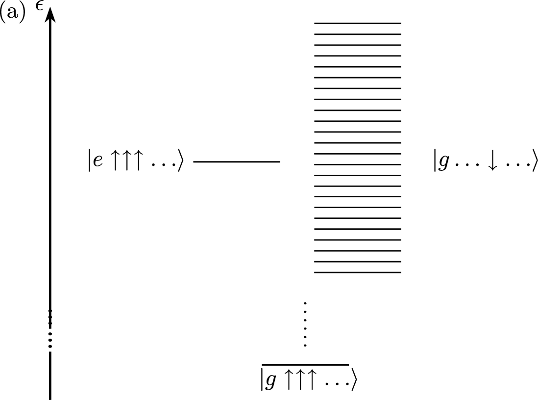
Our purpose is to diagonalize the Hamiltonian in the one-excitation subspace and to find the overlap of the initial state $\left|i\right\rangle$ (qubit excited, all fluctuators in the ground state) with the eigenstates $\left|\phi_{k}\right\rangle$, labeled by an index $k$ and having the eigenenergies $E_{k}$. This allows us to obtain the time evolution of the initial state:

We begin with the case of a completely uniform spectral distribution. This case is well known in quantum optics as the Wigner-Weisskopf theory [34]. We obtain a Lorentzian shape of the overlap function. Figure 9 shows the overlap $\left|\left\langle\phi_{k}|i\right\rangle\right|^{2}$ for an effective density $\bar{\nu}=1$ as a function of $E_{k}$. We arrive at the probability amplitude to find the qubit still excited after time $t>0$:

where $\Gamma=\frac{\pi}{2}\,\bar{\nu}\cdot v_{\perp}$. Thus the decay of the initially excited qubit in this situation is described by a simple exponential decay, $|\left\langle i|i(t)\right\rangle|^{2}=e^{-\Gamma t}$. The width $\Gamma$ of the Lorentzian in Fig. 9 determines the decay rate of the excited state.

Note, that we did not include here the coupling of either the qubit or the fluctuators to the dissipative baths. These couplings will broaden each of the eigenstates by an amount $\sim\gamma_{1}^{f}$. As long as this broadening is smaller than the resulting decay rate $\Gamma=\frac{\pi}{2}\,\bar{\nu}\cdot v_{\perp}$ (for strongly coupled fluctuators ($v_{\perp}\gg\gamma_{1}^{f}$) and $\bar{\nu}>1$ this is always the case), the dissipative broadening has little effect. Thus the system of the coupled qubit and fluctuators remains for a long time ($\sim 1/\gamma_{1}^{f}$) in the one-excitation subspace, but the qubit relaxes much faster and the energy resides in the fluctuators.

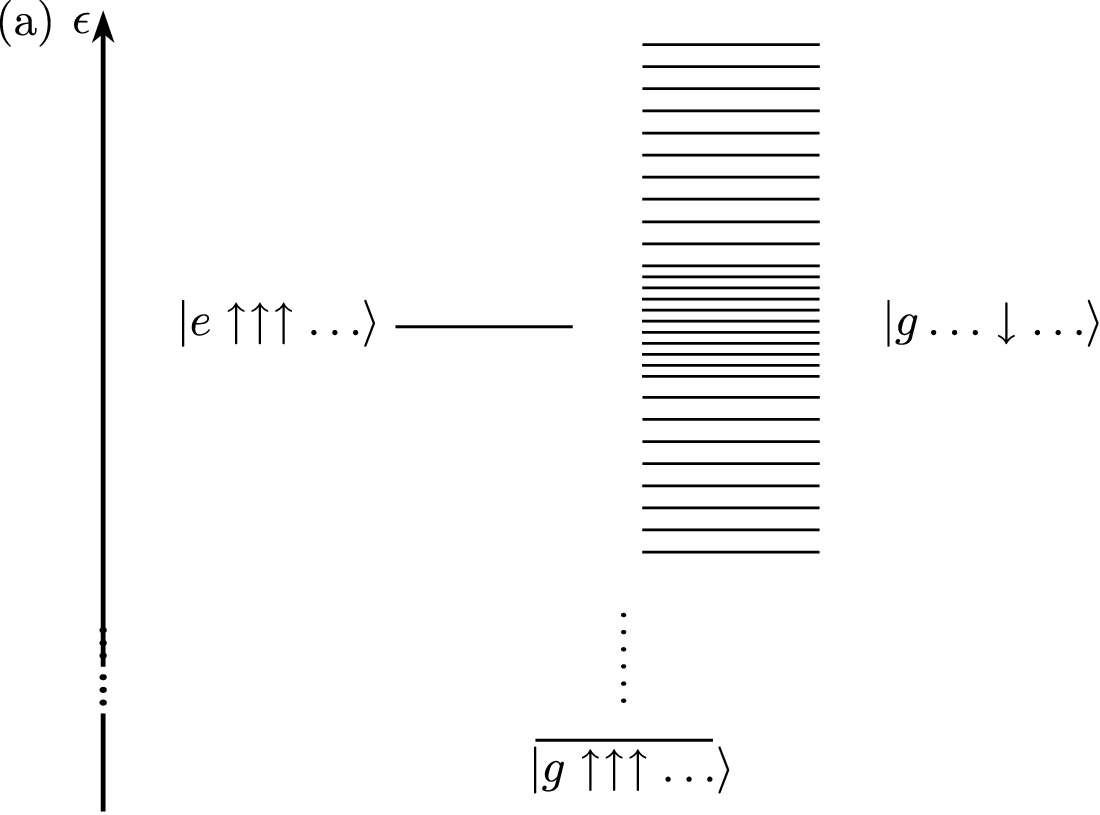
Further, we analyze the situation with a large number of TLFs, whose energy splittings are accumulated near some value. For instance, this behavior may originate from the microscopic nature of the fluctuators. As we have seen above, a collection of resonant TLFs is equivalent, within the single-excitation subspace, to one effective TLF with a much stronger coupling to the qubit. This results in two energy levels, separated by this new strong effective coupling constant. As we discussed above, this may be the origin of the visible properties of strongly coupled TLFs. To illustrate this setting, we show typical numerical results in Fig. 10. The data are shown for the situation, where instead of many resonant TLFs we have a large collection of TLFs distributed in a certain energy range. On top of the homogeneous distribution with density $\bar{\nu}=1$, we assume, locally, a higher density ($\bar{\nu}=10$) of fluctuators with energies close to that of the qubit. We obtain a double-peak structure for the overlap $\left|\left\langle\phi_{k}|i\right\rangle\right|^{2}$. Performing again a calculation of Eq. (36), we obtain oscillations with frequency given by the energy splitting of the two peaks in Fig. 10. The widths of the peaks (set at this level by the local density) determine the decay rate of the oscillations. If these peaks are wider than the dissipative broadening, the latter can be neglected. Thus, the effect of the fluctuator bath with strong density variations on the qubit is equivalent to that of a single TLF with an effective coupling strength $\tilde{v}_{\perp}$, much stronger than the couplings $v_{\perp,n}$ between the qubit and the individual physical TLFs.

References

- [1] G. Ithier, E. Collin, P. Joyez, P. J. Meeson, D. Vion, D. Esteve, F. Chiarello, A. Shnirman, Y. Makhlin, J. Schriefl, and G. Schön, Phys. Rev. B 72, 134519 (2005).
- [2] J. Koch, T. M. Yu, J. Gambetta, A. A. Houck, D. I. Schuster, J. Majer, A. Blais, M. H. Devoret, S. M. Girvin, and R. J. Schoelkopf, Phys. Rev. A 76, 042319 (2007a).
- [3] A. A. Houck, J. A. Schreier, B. R. Johnson, J. M. Chow, J. Koch, J. M. Gambetta, D. I. Schuster, L. Frunzio, M. H. Devoret, S. M. Girvin, et al., Phys. Rev. Lett. 101, 080502 (2008).
- [4] O. Astafiev, Y. A. Pashkin, Y. Nakamura, T. Yamamoto, and J. S. Tsai, Phys. Rev. Lett. 93, 267007 (2004).
- [5] D. J. Van Harlingen, T. L. Robertson, B. L. T. Plourde, P. A. Reichardt, T. A. Crane, and J. Clarke, Phys. Rev. B 70, 064517 (2004).
- [6] L. Faoro, J. Bergli, B. L. Altshuler, and Y. M. Galperin, Phys. Rev. Lett. 95, 046805 (2005).
- [7] L. Faoro and L. B. Ioffe, Phys. Rev. Lett. 96, 047001 (2006).
- [8] R. H. Koch, D. P. DiVincenzo, and J. Clarke, Phys. Rev. Lett. 98, 267003 (2007b).
- [9] L. Faoro and L. B. Ioffe, Phys. Rev. B 75, 132505 (2007).
- [10] A. Shnirman, G. Schön, I. Martin, and Y. Makhlin, Phys. Rev. Lett. 94, 127002 (2005).
- [11] P. Dutta and P. M. Horn, Rev. Mod. Phys. 53, 497 (1981).
- [12] L. Faoro and L. B. Ioffe, Phys. Rev. Lett. 100, 227005 (2008).
- [13] S. Sendelbach, D. Hover, A. Kittel, M. Mück, J. M. Martinis, and R. McDermott, Phys. Rev. Lett. 100, 227006 (2008).
- [14] R. W. Simmonds, K. M. Lang, D. A. Hite, S. Nam, D. P. Pappas, and J. M. Martinis, Phys. Rev. Lett. 93, 077003 (2004).
- [15] K. B. Cooper, M. Steffen, R. McDermott, R. W. Simmonds, S. Oh, D. A. Hite, D. P. Pappas, and J. M. Martinis, Phys. Rev. Lett. 93, 180401 (2004).
- [16] M. Neeley, M. Ansmann, R. C. Bialczak, M. Hofheinz, N. Katz, E. Lucero, A. O’Connel, H. Wang, A. N. Cleland, and J. M. Martinis, Nat. Phys. 4, 523 (2008).
- [17] A. M. Zagoskin, S. Ashhab, J. R. Johansson, and F. Nori, Phys. Rev. Lett. 97, 077001 (2006).
- [18] E. Paladino, L. Faoro, G. Falci, and R. Fazio, Phys. Rev. Lett. 88, 228304 (2002).
- [19] R. de Sousa, K. B. Whaley, F. K. Wilhelm, and J. von Delft, Phys. Rev. Lett. 95, 247006 (2005).
- [20] A. Grishin, I. V. Yurkevich, and I. V. Lerner, Phys. Rev. B 72, 060509 (R) (2005).
- [21] U. Weiss, Quantum Dissipative Systems (World Scientific, Singapore, 2008).
- [22] Y. Nakamura, private communication.
- [23] A. Lupascu, P. Bertet, E. F. C. Driessen, C. J. P. M. Harmans, and J. E. Mooij, arXiv:0810.0590 (2008).
- [24] M. Hofheinz, private communication.
- [25] J. Lisenfeld, private communication.
- [26] Y. M. Galperin, B. L. Altshuler, J. Bergli, and D. V. Shantsev, Phys. Rev. Lett. 96, 1 (2006).
- [27] J. Schriefl, Y. Makhlin, A. Shnirman, and G. Schön, New J. Phys. 8, 1 (2006).
- [28] F. Bloch, Phys. Rev. 105, 1206 (1957).
- [29] A. G. Redfield, IBM Journal of Research and Development 1, 19 (1957).
- [30] Y. Makhlin, G. Schön, and A. Shnirman, in New Directions in Mesoscopic Physics (Towards Nanoscience), edited by R. Fazio, V. F. Gantmakher, and Y. Imry (Kluwer, Dordrecht, 2003), pp. 197–224.
- [31] Y. Makhlin and A. Shnirman, Phys. Rev. Lett. 92, 178301 (2004).
- [32] S. Ashhab, J. R. Johansson, and F. Nori, Physica C 444, 45 (2006).
- [33] M. Hofheinz, H. Wang, M. Ansmann, R. C. Bialczak, E. Lucero, M. Neeley, A. D. O’Connell, D. Sank, J. Wenner, J. M. Martinis, et al., Nature 459, 546 (2009).
- [34] V. Weisskopf and E. Wigner, Z. Phys. 63, 54 (1930).