跳到论文正文
W Papers独立论文阅读器 arXiv:0905.2116 论文正文 计算阅读时间 · 0%
引用这篇论文根据当前论文元数据生成,正式投稿前建议核对。


License: arXiv.org perpetual non-exclusive license
arXiv:0905.2116v2 [math.GT] 15 Mar 2012

The homotopy and cohomology of spaces
of locally convex curves in the sphere — II

Nicolau C. Saldanha
Abstract

A smooth curve γ:[0,1]→𝕊2\gamma:[0,1]\to{\mathbb{S}}^{2} is locally convex if its geodesic curvature is positive at every point. J. A. Little showed that the space of all locally positive curves γ\gamma with γ⁡(0)=γ⁡(1)=e1\gamma(0)=\gamma(1)=e_{1} and γ′​(0)=γ′​(1)=e2\gamma^{\prime}(0)=\gamma^{\prime}(1)=e_{2} has three connected components ℒ−1,c{\cal L}_{-1,c}, ℒ+1{\cal L}_{+1}, ℒ−1,n{\cal L}_{-1,n}. The space ℒ−1,c{\cal L}_{-1,c} is known to be contractible but the topology of the other two connected components is not well understood. We prove that all connected components of ℒI{\cal L}_{I} are simply connected, that H2​(ℒ+1,ℤ)=ℤ2H^{2}({\cal L}_{+1};{\mathbb{Z}})={\mathbb{Z}}^{2} and H2​(ℒ−1,n,ℤ)=ℤH^{2}({\cal L}_{-1,n};{\mathbb{Z}})={\mathbb{Z}}.

1 Introduction

†† 2000 Mathematics Subject Classification. Primary 57N65, 53C42; Secondary 34B05. Keywords and phrases Convex curves, topology in infinite dimension, periodic solutions of linear ODEs.

A curve γ:[0,1]→𝕊2\gamma:[0,1]\to{\mathbb{S}}^{2} is called locally convex if its geodesic curvature is always positive, or, equivalently, if det(γ⁡(t),γ′​(t),γ′′​(t))>0\det(\gamma(t),\gamma^{\prime}(t),\gamma^{\prime\prime}(t))>0 for all tt. Let ℒI{\cal L}_{I} be the space of all locally convex curves γ\gamma with γ⁡(0)=γ⁡(1)=e1\gamma(0)=\gamma(1)=e_{1} and γ′​(0)=γ′​(1)=e2\gamma^{\prime}(0)=\gamma^{\prime}(1)=e_{2}. J. A. Little [2] showed that ℒI{\cal L}_{I} has three connected components ℒ−1,c{\cal L}_{-1,c}, ℒ+1{\cal L}_{+1}, ℒ−1,n{\cal L}_{-1,n}: we call these the Little spaces. Figure 1 shows examples of curves in ℒ−1,c{\cal L}_{-1,c}, ℒ+1{\cal L}_{+1} and ℒ−1,n{\cal L}_{-1,n}, respectively. The space ℒ−1,c{\cal L}_{-1,c} is known to be contractible ([7]) but the topology of the other two connected components is not well understood. In this series of papers we present new results concerning the homotopy and cohomology of the Little spaces. A more ambitious aim would be to determine the homotopy type of these spaces (which we hope to accomplish in [3]).

Refer to caption
Figure 1: Curves in ℒ−1,c{\cal L}_{-1,c}, ℒ+1{\cal L}_{+1} and ℒ−1,n{\cal L}_{-1,n}.

Let ℐI{\cal I}_{I} be the space of immersed curves γ:[0,1]→𝕊2\gamma:[0,1]\to{\mathbb{S}}^{2}, γ⁡(0)=γ⁡(1)=e1\gamma(0)=\gamma(1)=e_{1}, γ′​(0)=γ′​(1)=e2\gamma^{\prime}(0)=\gamma^{\prime}(1)=e_{2}. For each γ∈ℐI\gamma\in{\cal I}_{I}, consider its Frenet frame 𝔉γ:[0,1]→S​O​(3){\mathfrak{F}}_{\gamma}:[0,1]\to SO(3) and its lift 𝔉~γ:[0,1]→𝕊3\tilde{\mathfrak{F}}_{\gamma}:[0,1]\to{\mathbb{S}}^{3}. The value of 𝔉~γ​(1)\tilde{\mathfrak{F}}_{\gamma}(1) defines the two connected components of ℐI{\cal I}_{I}: γ∈ℐ+1\gamma\in{\cal I}_{+1} if and only if 𝔉~γ​(1)=1\tilde{\mathfrak{F}}_{\gamma}(1)=1. It is well know that each space ℐ±1{\cal I}_{\pm 1} is homotopically equivalent to Ω​𝕊3\Omega{\mathbb{S}}^{3}. In particular each ℐ±1{\cal I}_{\pm 1} is connected, simply connected and there is an element 𝐱∈H2​(ℐ±1,ℤ){\bf x}\in H^{2}({\cal I}_{\pm 1};{\mathbb{Z}}) such that each H2​k​(ℐ±1,ℤ)=ℤH^{2k}({\cal I}_{\pm 1};{\mathbb{Z}})={\mathbb{Z}} is generated by 𝐱k{\bf x}^{k}. Let ℒ+1=ℐ+1∩ℒI{\cal L}_{+1}={\cal I}_{+1}\cap{\cal L}_{I}, ℒ−1=ℒ−1,c⊔ℒ−1,n=ℐ−1∩ℒI{\cal L}_{-1}={\cal L}_{-1,c}\sqcup{\cal L}_{-1,n}={\cal I}_{-1}\cap{\cal L}_{I}. In the first paper ([4]) we saw that the inclusions ℒ±1⊂ℐ±1{\cal L}_{\pm 1}\subset{\cal I}_{\pm 1} are homotopically surjective but not homotopy equivalences. Indeed, we constructed elements 𝐟2​k∈H2​k​(ℒ(−1)(k+1),ℤ){\bf f}_{2k}\in H^{2k}({\cal L}_{(-1)^{(k+1)}};{\mathbb{Z}}) and maps 𝐠2​k:𝕊2​k→ℒ(−1)(k+1){\bf g}_{2k}:{\mathbb{S}}^{2k}\to{\cal L}_{(-1)^{(k+1)}} with 𝐟2​k​(𝐠2​k)=1{\bf f}_{2k}({\bf g}_{2k})=1, 𝐠2​k{\bf g}_{2k} homotopic to a constant in ℐ(−1)(k+1){\cal I}_{(-1)^{(k+1)}} and 𝐟2​k{\bf f}_{2k} not in (the image of) H2​k​(ℐ(−1)(k+1),ℤ)H^{2k}({\cal I}_{(-1)^{(k+1)}};{\mathbb{Z}}). In other words, there we give lower estimates for the groups H2​k​(ℒ±1,ℤ)H^{2k}({\cal L}_{\pm 1};{\mathbb{Z}}) and π2​k​(ℒ±1)\pi_{2k}({\cal L}_{\pm 1}). In the present paper we give upper estimates which imply the following theorem.

Theorem 1

The connected components of ℒI{\cal L}_{I} are simply connected. Furthermore, H2​(ℒ−1,n,ℤ)H^{2}({\cal L}_{-1,n};{\mathbb{Z}}) is generated by 𝐱{\bf x} and H2​(ℒ+1,ℤ)H^{2}({\cal L}_{+1};{\mathbb{Z}}) is generated by 𝐱{\bf x} and 𝐟2{\bf f}_{2}. Also, π2​(ℒ−1,n)=ℤ\pi_{2}({\cal L}_{-1,n})={\mathbb{Z}} and π2​(ℒ+1)=ℤ2\pi_{2}({\cal L}_{+1})={\mathbb{Z}}^{2} is generated by 𝐠2{\bf g}_{2} and 𝐠~2\tilde{\bf g}_{2}.

Notice that ℒp​e​r{\cal L}_{per}, the set of all 11-periodic locally convex curves γ~:ℝ→𝕊2\tilde{\gamma}:{\mathbb{R}}\to{\mathbb{S}}^{2} is homeomorphic to S​O​(3)×ℒISO(3)\times{\cal L}_{I}: define Ψ:ℒp​e​r→S​O​(3)×ℒI\Psi:{\cal L}_{per}\to SO(3)\times{\cal L}_{I} by Ψ⁡(γ~)=(𝔉γ~​(0),(𝔉γ~​(0))−1​γ~|[0,1])\Psi(\tilde{\gamma})=({\mathfrak{F}}_{\tilde{\gamma}}(0),({\mathfrak{F}}_{\tilde{\gamma}}(0))^{-1}\tilde{\gamma}|_{[0,1]}). We usually prefer to work in ℒI{\cal L}_{I} but sometimes move to ℒp​e​r{\cal L}_{per}.

In Section 2 we review some known results. Section 3 contains an algebraic description of the all-important construction Δ♯\Delta^{\sharp}; pulling one loop around is a special case of Δ♯\Delta^{\sharp}. Section 4 discusses the uses and limitations of Δ♯\Delta^{\sharp} to prove that a map f:K→ℒIf:K\to{\cal L}_{I} is homotopic to ν2∗f\nu_{2}\ast f (which essentially reduces the problem to the well-understood scenario of immersions). In Section 5 the discussion becomes more geometric and less algebraic as we discuss loops and the set 𝒯0⊂ℒ+1{\cal T}_{0}\subset{\cal L}_{+1} of stars: roughly, once 𝒯0{\cal T}_{0} is removed, ℒ+1∖𝒯0{\cal L}_{+1}\smallsetminus{\cal T}_{0} rather resembles ℐ+1{\cal I}_{+1}. Section 6 polishes a few nasty configurations so that we can complete the proof of our main results in Section 7. Section 8 is a very short conclusion.

The author would like to thank Dan Burghelea and Boris Shapiro for helpful conversations. The author acknowledges the hospitality of The Mathematics Department of The Ohio State University during the winter quarters of 2004 and 2009 and the support of CNPq, Capes and Faperj (Brazil).

2 Previous results

One of the fundamental constructions in Little’s argument is that if the curve γ∈ℒI\gamma\in{\cal L}_{I} has a loop, we can add a pair of loops as in Figure 2: in (a), the loop moves one full turn along a geodesic and in (b) the large loops are shrunk (we will discuss (c) later).

Refer to caption
Figure 2: How to go from γ\gamma to γ♯\gamma^{\sharp}

Let 𝒞0{\cal C}_{0} be the circle with diameter e1​e3e_{1}e_{3}, parametrized by ν1∈ℒI\nu_{1}\in{\cal L}_{I},

ν1​(t)=(1+cos⁡(2​π​t)2,22​sin⁡(2​π​t),1−cos⁡(2​π​t)2).\nu_{1}(t)=\left(\frac{1+\cos(2\pi t)}{2},\frac{\sqrt{2}}{2}\sin(2\pi t),\frac{1-\cos(2\pi t)}{2}\right).

For positive nn, let νn​(t)=ν1​(n​t)\nu_{n}(t)=\nu_{1}(nt) so that ν1∈ℒ−1,c\nu_{1}\in{\cal L}_{-1,c} and, for n>1n>1, νn∈ℒ(−1)n\nu_{n}\in{\cal L}_{(-1)^{n}}.

For γ1∈ℐσ1\gamma_{1}\in{\cal I}_{\sigma_{1}}, γ2∈ℐσ2\gamma_{2}\in{\cal I}_{\sigma_{2}}, σi∈{+1,−1}\sigma_{i}\in\{+1,-1\}, let γ1∗γ2∈ℐσ1​σ2\gamma_{1}\ast\gamma_{2}\in{\cal I}_{\sigma_{1}\sigma_{2}} be defined by

(γ1∗γ2)​(t)={γ1​(2​t),0≤t≤1/2,γ2​(2​t−1),1/2≤t≤1.(\gamma_{1}\ast\gamma_{2})(t)=\begin{cases}\gamma_{1}(2t),&0\leq t\leq 1/2,\\ \gamma_{2}(2t-1),&1/2\leq t\leq 1.\end{cases}

Notice that if γ1,γ2∈ℒI\gamma_{1},\gamma_{2}\in{\cal L}_{I} then γ1∗γ2∈ℒI\gamma_{1}\ast\gamma_{2}\in{\cal L}_{I}. For f:K→ℐIf:K\to{\cal I}_{I}, let νn∗f:K→ℐI\nu_{n}\ast f:K\to{\cal I}_{I} be defined by (νn∗f)​(p)=νn∗(f⁡(p))(\nu_{n}\ast f)(p)=\nu_{n}\ast(f(p)). Intuitively, νn∗f\nu_{n}\ast f is obtained from ff by adding nn loops to f⁡(p)f(p) at the point f​(p)​(0)f(p)(0). We may want to spread out nn loops along the curve: for γ∈ℐσ\gamma\in{\cal I}_{\sigma} and for large nn, define (Fn​(γ))​(t)=𝔉γ​(t)​νn​(t)(F_{n}(\gamma))(t)={\mathfrak{F}}_{\gamma}(t)\nu_{n}(t). For small nn, the above function from [0,1][0,1] to 𝕊2{\mathbb{S}}^{2} may not be an immersion. For sufficiently large nn, however, Fn​(γ)∈ℒ(−1)n​σF_{n}(\gamma)\in{\cal L}_{(-1)^{n}\sigma}.

By the above construction, it is clear that given γ∈ℒ+1⊔ℒ−1,n\gamma\in{\cal L}_{+1}\sqcup{\cal L}_{-1,n} there exist Ha,Hb:[0,1]→ℒ±1H_{a},H_{b}:[0,1]\to{\cal L}_{\pm 1}, Ha​(0)=Hb​(0)=γH_{a}(0)=H_{b}(0)=\gamma, Ha​(1)=ν2∗γH_{a}(1)=\nu_{2}\ast\gamma, Hb​(1)=F2​n​(γ)H_{b}(1)=F_{2n}(\gamma). The construction is not uniform, however: is depends on the choice of the loop. In other words, given a compact set KK and a map f:K→ℒ+1⊔ℒ−1,nf:K\to{\cal L}_{+1}\sqcup{\cal L}_{-1,n}, the existence of H:[0,1]×K→ℒ+1⊔ℒ−1,nH:[0,1]\times K\to{\cal L}_{+1}\sqcup{\cal L}_{-1,n}, H⁡(0,⋅)=fH(0,\cdot)=f, H⁡(1,⋅)=ν2∗fH(1,\cdot)=\nu_{2}\ast f or H⁡(1,⋅)=F2​n∘fH(1,\cdot)=F_{2n}\circ f is not clear at this point. Indeed, the existence (or not) of such a homotopy is the crucial point in this paper. The following proposition helps clarify the situation.

Proposition 2.1 ([4])

Let KK be a compact set and let f:K→ℒI⊂ℐIf:K\to{\cal L}_{I}\subset{\cal I}_{I} a continuous function.

  1. (a)

    For sufficiently large nn, the functions ν2∗f\nu_{2}\ast f and F2​n∘fF_{2n}\circ f are homotopic in ℒI{\cal L}_{I}.

  2. (b)

    If f=ν1∗f~f=\nu_{1}\ast\tilde{f} (for some f~\tilde{f}) then ff is homotopic to ν2∗f\nu_{2}\ast f.

  3. (c)

    The function ff is homotopic to a constant in ℐI{\cal I}_{I} if and only if ν2∗f\nu_{2}\ast f is homotopic to a constant in ℒI{\cal L}_{I}.

  4. (d)

    There exists a map 𝐠2:𝕊2→ℒ+1{\bf g}_{2}:{\mathbb{S}}^{2}\to{\cal L}_{+1} such that ν2∗𝐠2\nu_{2}\ast{\bf g}_{2} is homotopic to a constant in ℒ+1{\cal L}_{+1} but 𝐠2{\bf g}_{2} is not.

3 Bruhat cells and the set 𝒲{\cal W}

Given a locally convex curve γ:[0,1]→𝕊2\gamma:[0,1]\to{\mathbb{S}}^{2} and a 3×33\times 3 matrix AA with positive determinant, the curve γA:[0,1]→𝕊2\gamma^{A}:[0,1]\to{\mathbb{S}}^{2},

γA​(t)=A​γ​(t)|A​γ​(t)|\gamma^{A}(t)=\frac{A\gamma(t)}{|A\gamma(t)|}

is also locally convex. Furthermore, 𝔉γA​(t)=A​𝔉γ​(t)​U{\mathfrak{F}}_{\gamma^{A}}(t)=A{\mathfrak{F}}_{\gamma}(t)U for U∈𝒰+U\in{\cal U}^{+}, where 𝒰+{\cal U}^{+} is the group of upper triangular 3×33\times 3 matrices with positive off-diagonal entries.

Let 𝒰1⊂𝒰+{\cal U}^{1}\subset{\cal U}^{+} be the group of upper triangular matrices with unit diagonal. Recall that S​O​(3)SO(3) is divided in Bruhat cells by the following equivalence relation: Q1Q_{1} and Q2Q_{2} are equivalent if and only if there exist U1∈𝒰1U_{1}\in{\cal U}^{1} and U2∈𝒰+U_{2}\in{\cal U}^{+} with Q1=U1​Q2​U2Q_{1}=U_{1}Q_{2}U_{2}. The group Weyl group D3⊂S​O​(3)D_{3}\subset SO(3) of signed permutation matrices with positive determinant has one element per cell. The four open cells 𝒥1,𝒥2,𝒥3,𝒥4{\cal J}_{1},{\cal J}_{2},{\cal J}_{3},{\cal J}_{4} have respective representatives

J1=(00−1010100),J2=(0010−10100),\displaystyle J_{1}=\begin{pmatrix}0&0&-1\\ 0&1&0\\ 1&0&0\end{pmatrix},\quad J_{2}=\begin{pmatrix}0&0&1\\ 0&-1&0\\ 1&0&0\end{pmatrix},
J3=(001010−100),J4=(00−10−10−100).\displaystyle J_{3}=\begin{pmatrix}0&0&1\\ 0&1&0\\ -1&0&0\end{pmatrix},\quad J_{4}=\begin{pmatrix}0&0&-1\\ 0&-1&0\\ -1&0&0\end{pmatrix}.

Further recall ([6], [7], [5]) that given Q∈S​O​(3)Q\in SO(3) there exists a convex curve γ:[0,1]\gamma:[0,1] with 𝔉γ​(0)=I{\mathfrak{F}}_{\gamma}(0)=I and 𝔉γ​(1)=Q{\mathfrak{F}}_{\gamma}(1)=Q if and only if QQ belongs to 𝒥2{\cal J}_{2} or to one of the 55 lower dimensional cells in its boundary corresponding to the following matrices:

(100010001),(010−100001),(1000010−10),(001−1000−10),(010001100).\begin{pmatrix}1&0&0\\ 0&1&0\\ 0&0&1\end{pmatrix},\quad\begin{pmatrix}0&1&0\\ -1&0&0\\ 0&0&1\end{pmatrix},\quad\begin{pmatrix}1&0&0\\ 0&0&1\\ 0&-1&0\end{pmatrix},\quad\begin{pmatrix}0&0&1\\ -1&0&0\\ 0&-1&0\end{pmatrix},\quad\begin{pmatrix}0&1&0\\ 0&0&1\\ 1&0&0\end{pmatrix}.

As a consequence, given Q∈S​O​(3)Q\in SO(3), there exists γ∈ℒ−1,c\gamma\in{\cal L}_{-1,c} with 𝔉γ​(1/2)=Q{\mathfrak{F}}_{\gamma}(1/2)=Q if and only if Q∈𝒥2Q\in{\cal J}_{2}. Similarly, Q0−1​Q1∈𝒥4Q_{0}^{-1}Q_{1}\in{\cal J}_{4} if and only if there exists a convex curve γ:[0,1]→𝕊2\gamma:[0,1]\to{\mathbb{S}}^{2} with γ⁡(0)=γ⁡(1)=Q0​e1\gamma(0)=\gamma(1)=Q_{0}e_{1}, γ′​(0)=γ′​(1)=−Q0​e2\gamma^{\prime}(0)=\gamma^{\prime}(1)=-Q_{0}e_{2}, γ⁡(1/2)=Q1​e1\gamma(1/2)=Q_{1}e_{1}, γ′​(1/2)=−Q1​e2\gamma^{\prime}(1/2)=-Q_{1}e_{2}.

Let 𝒲⊂ℒI×𝕊1×𝕊1{\cal W}\subset{\cal L}_{I}\times{\mathbb{S}}^{1}\times{\mathbb{S}}^{1} be the set of triples (γ,t0,t1)(\gamma,t_{0},t_{1}) such that (𝔉γ​(t0))−1​𝔉γ​(t1)∈𝒥4({\mathfrak{F}}_{\gamma}(t_{0}))^{-1}{\mathfrak{F}}_{\gamma}(t_{1})\in{\cal J}_{4}. Define U1:𝒲→𝒰1U_{1}:{\cal W}\to{\cal U}^{1} and U2:𝒲→𝒰+U_{2}:{\cal W}\to{\cal U}^{+} so that (𝔉γ​(t0))−1​𝔉γ​(t1)=U1​J4​U2({\mathfrak{F}}_{\gamma}(t_{0}))^{-1}{\mathfrak{F}}_{\gamma}(t_{1})=U_{1}J_{4}U_{2}. Alternatively, (γ,t0,t1)∈𝒲(\gamma,t_{0},t_{1})\in{\cal W} if and only if there exists a convex curve α:𝕊1→𝕊2\alpha:{\mathbb{S}}^{1}\to{\mathbb{S}}^{2}, α⁡(0)=γ⁡(t0)\alpha(0)=\gamma(t_{0}), α′​(0)=−γ′​(t0)\alpha^{\prime}(0)=-\gamma^{\prime}(t_{0}), α⁡(1)=γ⁡(t1)\alpha(1)=\gamma(t_{1}), α′​(1)=−γ′​(t1)\alpha^{\prime}(1)=-\gamma^{\prime}(t_{1}). Notice that 𝒲{\cal W} is an open subset of ℒI×𝕊1×𝕊1{\cal L}_{I}\times{\mathbb{S}}^{1}\times{\mathbb{S}}^{1}; (γ,t0,t1)∈𝒲(\gamma,t_{0},t_{1})\in{\cal W} implies t0≠t1t_{0}\neq t_{1} and (γ,t1,t0)∈𝒲(\gamma,t_{1},t_{0})\in{\cal W}.

We now define the function Δ♯:[0,+∞)×𝒲→ℒI\Delta^{\sharp}:[0,+\infty)\times{\cal W}\to{\cal L}_{I}, one of our main technical tools throughout the paper.

Definition 3.1

Let (γ,t0,t1)∈𝒲(\gamma,t_{0},t_{1})\in{\cal W} and t∙∈𝕊1t_{\bullet}\in{\mathbb{S}}^{1} with t∙<t0<t1<t∙+1t_{\bullet}<t_{0}<t_{1}<t_{\bullet}+1. Take ϵ♯>0\epsilon^{\sharp}>0, ϵ♯<(1/20)​min⁡(t0−t∙,t1−t0,t∙+1−t1)\epsilon^{\sharp}<(1/20)\min(t_{0}-t_{\bullet},t_{1}-t_{0},t_{\bullet}+1-t_{1}). Let Q0=𝔉γ​(t0)Q_{0}={\mathfrak{F}}_{\gamma}(t_{0}), Q1=𝔉γ​(t1)Q_{1}={\mathfrak{F}}_{\gamma}(t_{1}), U1=U1​(γ,t0,t1)U_{1}=U_{1}(\gamma,t_{0},t_{1}), U2=U2​(γ,t0,t1)U_{2}=U_{2}(\gamma,t_{0},t_{1}) so that Q0−1​Q1=U1​J4​U2Q_{0}^{-1}Q_{1}=U_{1}J_{4}U_{2}. Let α=γU1−1​Q0−1\alpha=\gamma^{U_{1}^{-1}Q_{0}^{-1}}, i.e.,

α⁡(t)=U1−1​Q0−1​γ​(t)|U1−1​Q0−1​γ​(t)|;\alpha(t)=\frac{U_{1}^{-1}Q_{0}^{-1}\gamma(t)}{|U_{1}^{-1}Q_{0}^{-1}\gamma(t)|};

α\alpha is locally convex with 𝔉α​(t0)=I{\mathfrak{F}}_{\alpha}(t_{0})=I, 𝔉α​(t1)=J4{\mathfrak{F}}_{\alpha}(t_{1})=J_{4}. For s∈[0,+∞)s\in[0,+\infty), let Ts=min⁡(s,2)T_{s}=\min(s,2); define an increasing piecewise linear homeomorphisms ha,s:[0,Ts​ϵ♯]→[0,s]h_{a,s}:[0,T_{s}\epsilon^{\sharp}]\to[0,s] whose graph is a polygonal line with vertices (0,0)(0,0), (ϵ♯,1)(\epsilon^{\sharp},1) (if s≥1s\geq 1) and (Ts​ϵ♯,s)(T_{s}\epsilon^{\sharp},s). Similarly, let the graph of hb,s:[t0+ϵ♯​Ts,t1−ϵ♯​Ts]→[t0,t1]h_{b,s}:[t_{0}+\epsilon^{\sharp}T_{s},t_{1}-\epsilon^{\sharp}T_{s}]\to[t_{0},t_{1}] have vertices (t0+Ts​ϵ♯,t0)(t_{0}+T_{s}\epsilon^{\sharp},t_{0}), (t0+4​ϵ♯,t0+4​ϵ♯)(t_{0}+4\epsilon^{\sharp},t_{0}+4\epsilon^{\sharp}) (t1−4​ϵ♯,t1−4​ϵ♯)(t_{1}-4\epsilon^{\sharp},t_{1}-4\epsilon^{\sharp}) and (t1−Ts​ϵ♯,t1)(t_{1}-T_{s}\epsilon^{\sharp},t_{1}). Define αs:[t0,t1]→𝕊2\alpha_{s}:[t_{0},t_{1}]\to{\mathbb{S}}^{2} by

αs​(t)={ν1​(ha,s​(t−t0)),t0≤t≤t0+Ts​ϵ♯,𝔉ν1​(s)​α​(hb,s​(t)),t0+Ts​ϵ♯≤t≤t1−Ts​ϵ♯,J4​ν1​(−ha,s​(t1−t)),t1−Ts​ϵ♯≤t≤t1.\alpha_{s}(t)=\begin{cases}\nu_{1}\left(h_{a,s}(t-t_{0})\right),&t_{0}\leq t\leq t_{0}+T_{s}\epsilon^{\sharp},\\ {\mathfrak{F}}_{\nu_{1}}(s)\alpha\left(h_{b,s}(t)\right),&t_{0}+T_{s}\epsilon^{\sharp}\leq t\leq t_{1}-T_{s}\epsilon^{\sharp},\\ J_{4}\nu_{1}\left(-h_{a,s}(t_{1}-t)\right),&t_{1}-T_{s}\epsilon^{\sharp}\leq t\leq t_{1}.\end{cases}

Finally,

Q​Δ♯​(s,γ,t0,t1)={γ⁡(t),t∙≤t≤t0​ or ​t1≤t≤t∙,(αs)Q0​U1​(t),t0≤t≤t1,Q\Delta^{\sharp}(s,\gamma,t_{0},t_{1})=\begin{cases}\gamma(t),&t_{\bullet}\leq t\leq t_{0}\textrm{ or }t_{1}\leq t\leq t_{\bullet},\\ (\alpha_{s})^{Q_{0}U_{1}}(t),&t_{0}\leq t\leq t_{1},\end{cases}

where Q∈S​O​(3)Q\in SO(3) is uniquely chosen so that 𝔉Δ♯​(s,γ,t0,t1)​(0)=I{\mathfrak{F}}_{\Delta^{\sharp}(s,\gamma,t_{0},t_{1})}(0)=I.

A few remarks are in order. The curve αs\alpha_{s} is obtained from α\alpha by attaching an arc of circle of angle 2​π​s2\pi s to either end, rotating the curve to keep the same endpoints and reparametrizing. Similarly, Δ♯​(s,γ,t0,t1)\Delta^{\sharp}(s,\gamma,t_{0},t_{1}) is obtained from γ\gamma by inserting an arc of 2​π​s2\pi s at positions t0t_{0} and t1t_{1}; if ss is not an integer, the portion of γ\gamma between t0t_{0} and t1t_{1} will be “rotated”. Up to minor deformations, the path Δ♯​(s,γ,t0,t1)\Delta^{\sharp}(s,\gamma,t_{0},t_{1}), s∈[0,1]s\in[0,1], from γ\gamma to γt0,t1♯=Δ♯​(1,γ,t0,t1)\gamma^{\sharp}_{t_{0},t_{1}}=\Delta^{\sharp}(1,\gamma,t_{0},t_{1}) is exemplified in Figure 2 (in a situation where 0<t0<t1<10<t_{0}<t_{1}<1). The loop between t0t_{0} and t1t_{1} is pushed along a geodesic all the way, until it comes back (a). The two long chunks of curve (in the figure, very nearly geodesics) are then shrunk (b) and rounded (c) so that we obtain γt0,t1♯\gamma^{\sharp}_{t_{0},t_{1}}. Notice that the portion of γ\gamma outside the interval [t0,t1][t_{0},t_{1}] is unaltered throughout the process.

Strictly speaking, the definition of Δ♯\Delta^{\sharp} depends on the choice of ϵ♯\epsilon^{\sharp}: the only difference, however, when you change ϵ♯\epsilon^{\sharp} is that functions get reparametrized. Similarly, we ask that U1∈𝒰1U_{1}\in{\cal U}^{1} so that U1U_{1} and U2U_{2} become uniquely determined. The function hsh_{s} in Definition 3.1 is chosen so that the following technical result holds.

Lemma 3.2

Let KK be a compact set and (f,t0,t1):K→𝒲(f,t_{0},t_{1}):K\to{\cal W} a continuous map; there exists ϵ♯>0\epsilon^{\sharp}>0 which suits the definition of Δ♯​(s,f⁡(p),t0​(p),t1​(p))\Delta^{\sharp}(s,f(p),t_{0}(p),t_{1}(p)) for all ss.

Let 𝒦⊂ℒI{\cal K}\subset{\cal L}_{I} be the compact set of all curves of the form Δ♯​(s,f⁡(p),t0​(p),t1​(p))\Delta^{\sharp}(s,f(p),t_{0}(p),t_{1}(p)), p∈Kp\in K, s∈[0,3]s\in[0,3]. For s>0s>0, let n=⌊s−3⌋n=\lfloor s-3\rfloor, s~=s−n\tilde{s}=s-n. For p∈Kp\in K, let γ=Δ♯​(s,f⁡(p),t0​(p),t1​(p))\gamma=\Delta^{\sharp}(s,f(p),t_{0}(p),t_{1}(p)), γ~=Δ♯​(s~,f⁡(p),t0​(p),t1​(p))\tilde{\gamma}=\Delta^{\sharp}(\tilde{s},f(p),t_{0}(p),t_{1}(p)). Let

h⁡(t)={0,t∙≤t≤t0,n⁡(t−t0)/ϵ♯,t0≤t≤t0+ϵ♯,n,t0+ϵ♯≤t≤t1−ϵ♯,2​n−n⁡(t1−t)/ϵ♯,t1−ϵ♯≤t≤t1,2​n,t1≤t≤t∙.h(t)=\begin{cases}0,&t_{\bullet}\leq t\leq t_{0},\\ n(t-t_{0})/{\epsilon^{\sharp}},&t_{0}\leq t\leq t_{0}+\epsilon^{\sharp},\\ n,&t_{0}+\epsilon^{\sharp}\leq t\leq t_{1}-\epsilon^{\sharp},\\ 2n-n(t_{1}-t)/{\epsilon^{\sharp}},&t_{1}-\epsilon^{\sharp}\leq t\leq t_{1},\\ 2n,&t_{1}\leq t\leq t_{\bullet}.\end{cases}

Then γ~∈𝒦\tilde{\gamma}\in{\cal K} and

γ⁡(t)=Q​𝔉γ~​(t)​ν1U1​(p)​(h⁡(t)),Q∈S​O​(3),\gamma(t)=Q{\mathfrak{F}}_{\tilde{\gamma}}(t)\nu^{U_{1}(p)}_{1}(h(t)),\quad Q\in SO(3),

where U1​(p)=U1​(f⁡(p),t0​(p),t1​(p))U_{1}(p)=U_{1}(f(p),t_{0}(p),t_{1}(p)).

Proof: This is a straightforward computation.     ■\blacksquare

The functions Δ♯​(s~,(Δ♯​(s,γ,t0,t1),t0,t1))\Delta^{\sharp}(\tilde{s},(\Delta^{\sharp}(s,\gamma,t_{0},t_{1}),t_{0},t_{1})) and Δ♯​(s+s~,γ,t0,t1)\Delta^{\sharp}(s+\tilde{s},\gamma,t_{0},t_{1}) differ by reparametrization only. Under suitable hypothesis, a related identity holds for distinct points (γ,t0,t1)(\gamma,t_{0},t_{1}), (γ,t2,t3)(\gamma,t_{2},t_{3}). Two points (γ,t0,t1),(γ,t2,t3)∈𝒲(\gamma,t_{0},t_{1}),(\gamma,t_{2},t_{3})\in{\cal W} are disjoint if the intervals [t0,t1],[t2,t3]⊂𝕊1[t_{0},t_{1}],[t_{2},t_{3}]\subset{\mathbb{S}}^{1} are disjoint, or, equivalently, if t0<t1<t2<t3<t0+1t_{0}<t_{1}<t_{2}<t_{3}<t_{0}+1 or t2<t3<t0<t1<t2+1t_{2}<t_{3}<t_{0}<t_{1}<t_{2}+1.

Lemma 3.3

If (γ,t0,t1),(γ,t2,t3)∈𝒲(\gamma,t_{0},t_{1}),(\gamma,t_{2},t_{3})\in{\cal W} are disjoint then, for any s,s~∈[0,1]s,\tilde{s}\in[0,1],

(Δ♯​(s,γ,t0,t1),t2,t3),(Δ♯​(s~,γ,t2,t3),t0,t1)∈𝒲.(\Delta^{\sharp}(s,\gamma,t_{0},t_{1}),t_{2},t_{3}),(\Delta^{\sharp}(\tilde{s},\gamma,t_{2},t_{3}),t_{0},t_{1})\in{\cal W}.

Furthermore,

Δ♯​(s~,(Δ♯​(s,γ,t0,t1),t2,t3))=Δ♯​(s,(Δ♯​(s~,γ,t2,t3),t0,t1)).\Delta^{\sharp}(\tilde{s},(\Delta^{\sharp}(s,\gamma,t_{0},t_{1}),t_{2},t_{3}))=\Delta^{\sharp}(s,(\Delta^{\sharp}(\tilde{s},\gamma,t_{2},t_{3}),t_{0},t_{1})).

Proof: This follows directly from the construction of Δ♯\Delta^{\sharp} and of the function γs∗\gamma^{\ast}_{s} in the definition. Indeed, γs∗\gamma^{\ast}_{s} for (t0,t1)(t_{0},t_{1}) coincides with γ\gamma in an open interval containing (t2,t3)(t_{2},t_{3}) (and vice versa).     ■\blacksquare

4 Disjoint covers

Recall that one of our aims is to decide whether a continuous map f:K→ℒIf:K\to{\cal L}_{I} is homotopic to ν2∗f\nu_{2}\ast f. In this section, we present several situations where this is the case and one example where this is not the case. We start with a simple example.

Lemma 4.1

Let KK be a compact set and f:K→ℒIf:K\to{\cal L}_{I} a continuous map. If there is a continuous function t1:K→𝕊1t_{1}:K\to{\mathbb{S}}^{1} such that for all p∈Kp\in K we have (f⁡(p),0,t1​(p))∈𝒲(f(p),0,t_{1}(p))\in{\cal W} then ff is homotopic to ν2∗f\nu_{2}\ast f.

Proof: Let H:[0,1]×K→ℒIH:[0,1]\times K\to{\cal L}_{I} be defined by H⁡(s,p)=Δ♯​(2​s,f⁡(p),0,t1​(p))H(s,p)=\Delta^{\sharp}(2s,f(p),0,t_{1}(p)). Up to reparametrization, H⁡(1,p)=ν2∗f~​(p)H(1,p)=\nu_{2}\ast\tilde{f}(p), where f~​(p)\tilde{f}(p) is obtained from f⁡(p)f(p) by inserting two turns at t1​(p)t_{1}(p). Since ν2\nu_{2} and ν4\nu_{4} are in the same connected component, ν2∗f~\nu_{2}\ast\tilde{f} is homotopic to ν2∗(ν2∗f~)\nu_{2}\ast(\nu_{2}\ast\tilde{f}) and therefore to ν2∗f\nu_{2}\ast f.     ■\blacksquare

Given this result, some questions are natural:

  • •

    If there exist continuous functions t0,t1:K→𝕊1t_{0},t_{1}:K\to{\mathbb{S}}^{1} with (f⁡(p),t0​(p),t1​(p))∈𝒲(f(p),t_{0}(p),t_{1}(p))\in{\cal W}, does it follow that ff is homotopic to ν2∗f\nu_{2}\ast f?

  • •

    If for every pp there exist t0,t1∈𝕊1t_{0},t_{1}\in{\mathbb{S}}^{1} such that (f⁡(p),t0,t1)∈𝒲(f(p),t_{0},t_{1})\in{\cal W}, does it follow that ff is homotopic to ν2∗f\nu_{2}\ast f?

As we shall see, the answers are yes and no, respectively. Before we attack these problems, however, we introduce a few concepts.

Define

𝒪={γ∈ℒI|∀t0,t1∈𝕊1,(γ,t0,t1)∉𝒲}:{\cal O}=\{\gamma\in{\cal L}_{I}\;|\;\forall t_{0},t_{1}\in{\mathbb{S}}^{1},(\gamma,t_{0},t_{1})\notin{\cal W}\}:

the set 𝒪{\cal O} is clearly a closed subset of ℒI{\cal L}_{I}. A double point of a curve γ∈ℒI\gamma\in{\cal L}_{I} is a pair (t0,t1)∈(𝕊1)2(t_{0},t_{1})\in({\mathbb{S}}^{1})^{2}, t0≠t1t_{0}\neq t_{1}, with γ⁡(t0)=γ⁡(t1)\gamma(t_{0})=\gamma(t_{1}). Similarly, an nn-tuple point is an nn-tuple (t0,t1,…,tn−1)(t_{0},t_{1},\ldots,t_{n-1}), 0≤t0<t1<⋯<tn−1<10\leq t_{0}<t_{1}<\cdots<t_{n-1}<1, such that γ⁡(t0)=γ⁡(t1)=⋯=γ⁡(tn−1)\gamma(t_{0})=\gamma(t_{1})=\cdots=\gamma(t_{n-1}). We identify the double point (t1,t0)(t_{1},t_{0}) with (t0,t1)(t_{0},t_{1}). A double point (t0,t1)(t_{0},t_{1}) is a self-tangency if γ′​(t0)\gamma^{\prime}(t_{0}) and γ′​(t1)\gamma^{\prime}(t_{1}) are parallel and transversal otherwise. A self-tangency (t0,t1)(t_{0},t_{1}) is positive if γ′​(t1)\gamma^{\prime}(t_{1}) is a positive multiple of γ′​(t0)\gamma^{\prime}(t_{0}) (and negative otherwise).

If (t0,t1)(t_{0},t_{1}) is a positive self-tangency, the normal vector 𝐧γ​(t)=𝔉γ​(t)​e3{\bf n}_{\gamma}(t)={\mathfrak{F}}_{\gamma}(t)e_{3} satisfies 𝐧γ​(t0)=𝐧γ​(t1){\bf n}_{\gamma}(t_{0})={\bf n}_{\gamma}(t_{1}). Define h1​(t)=⟨γ⁡(t),𝔉γ​(t)​e2⟩h_{1}(t)=\langle\gamma(t),{\mathfrak{F}}_{\gamma}(t)e_{2}\rangle, h2​(t)=⟨γ⁡(t),𝐧γ​(t0)⟩h_{2}(t)=\langle\gamma(t),{\bf n}_{\gamma}(t_{0})\rangle: notice that h1​(t0)=h1​(t1)=h2​(t0)=h2​(t1)=0h_{1}(t_{0})=h_{1}(t_{1})=h_{2}(t_{0})=h_{2}(t_{1})=0, h2′​(t0)=h2′​(t1)=0h_{2}^{\prime}(t_{0})=h_{2}^{\prime}(t_{1})=0, h1′​(t0)>0h_{1}^{\prime}(t_{0})>0 and h1′​(t1)>0h_{1}^{\prime}(t_{1})>0. There exists ϵ>0\epsilon>0 such that h1|(t0−ϵ,t0+ϵ)h_{1}|_{(t_{0}-\epsilon,t_{0}+\epsilon)} and h1|(t1−ϵ,t1+ϵ)h_{1}|_{(t_{1}-\epsilon,t_{1}+\epsilon)} are invertible. Let g0=h2∘(h1|(t0−ϵ,t0+ϵ))−1g_{0}=h_{2}\circ(h_{1}|_{(t_{0}-\epsilon,t_{0}+\epsilon)})^{-1} and g1=h2∘(h1|(t1−ϵ,t1+ϵ))−1g_{1}=h_{2}\circ(h_{1}|_{(t_{1}-\epsilon,t_{1}+\epsilon)})^{-1}: near the origin, the graph of gig_{i} is the orthogonal projection of the image of the curve γ\gamma near γ⁡(ti)\gamma(t_{i}) to the tangent plane, using γ′​(ti)/|γ′​(ti)|\gamma^{\prime}(t_{i})/|\gamma^{\prime}(t_{i})| and 𝐧γ​(ti){\bf n}_{\gamma}(t_{i}) as basis. By construction, g0​(0)=g1​(0)=0g_{0}(0)=g_{1}(0)=0 and g0′​(0)=g1′​(0)=0g_{0}^{\prime}(0)=g_{1}^{\prime}(0)=0. By convexity, g0′′​(0)>0g_{0}^{\prime\prime}(0)>0, g1′′​(0)>0g_{1}^{\prime\prime}(0)>0. The self-tangency (t0,t1)(t_{0},t_{1}) has order nn if g0(n)​(0)≠g1(n)​(0)g_{0}^{(n)}(0)\neq g_{1}^{(n)}(0) but g0(j)​(0)=g1(j)​(0)g_{0}^{(j)}(0)=g_{1}^{(j)}(0) for any j<nj<n and order +∞+\infty if g0(j)​(0)=g1(j)​(0)g_{0}^{(j)}(0)=g_{1}^{(j)}(0) for any jj. A self-osculating point is a positive self-tangency of order 33 or more.

Lemma 4.2

Let (t0,t1)(t_{0},t_{1}) be a double point of γ∈ℒI\gamma\in{\cal L}_{I}. If (t0,t1)(t_{0},t_{1}) is either transversal or a negative self-tangency then for any ϵ>0\epsilon>0 there exist t~0,t~1\tilde{t}_{0},\tilde{t}_{1}, |t~0−t0|+|t~1−t1|<ϵ|\tilde{t}_{0}-t_{0}|+|\tilde{t}_{1}-t_{1}|<\epsilon, (γ,t0,t1)∈𝒲(\gamma,t_{0},t_{1})\in{\cal W}.

Proof: First consider transversal double points. Assume without loss of generality that det(γ⁡(t0),γ′​(t0),γ′​(t1))>0\det(\gamma(t_{0}),\gamma^{\prime}(t_{0}),\gamma^{\prime}(t_{1}))>0. For small ϵ\epsilon we may take t~0=t0+ϵ/4\tilde{t}_{0}=t_{0}+\epsilon/4, t~1=t1−ϵ/4\tilde{t}_{1}=t_{1}-\epsilon/4: this is a straightforward computation but is probably best verified geometrically in Figure 3: the dashed convex curves tangent to γ\gamma validate the geometric characterization of 𝒲{\cal W}.

Refer to caption
Figure 3: Obtaining (t~0,t~1)(\tilde{t}_{0},\tilde{t}_{1}) such that (γ,t~0,t~1)∈𝒲(\gamma,\tilde{t}_{0},\tilde{t}_{1})\in{\cal W}.

For a negative self-tangency and small ϵ\epsilon we may take either t~0=t0+ϵ/4\tilde{t}_{0}=t_{0}+\epsilon/4, t~1=t1−ϵ/4\tilde{t}_{1}=t_{1}-\epsilon/4 or t~0=t0−ϵ/4\tilde{t}_{0}=t_{0}-\epsilon/4, t~1=t1+ϵ/4\tilde{t}_{1}=t_{1}+\epsilon/4: this is again verified in Figure 3.     ■\blacksquare

It follows directly from this result that if γ∈𝒪\gamma\in{\cal O} then all double points of γ\gamma are positive self-tangencies.

Refer to caption
Figure 4: A curve in 𝒪2{\cal O}_{2}.

The following proposition settles the second question raised at the beginning of this section. Recall ([4]) that 𝐠+,2:𝕊2→ℒ+1{\bf g}_{+,2}:{\mathbb{S}}^{2}\to{\cal L}_{+1} is an explicit function such that 𝐠+,2{\bf g}_{+,2} and ν2∗𝐠+,2\nu_{2}\ast{\bf g}_{+,2} are not homotopic in ℒ+1{\cal L}_{+1} (even though they are homotopic in ℐ+1{\cal I}_{+1}).

Proposition 4.3

There is a map f:𝕊2→ℒ+1∖𝒪f:{\mathbb{S}}^{2}\to{\cal L}_{+1}\smallsetminus{\cal O} which is homotopic (in ℒ+1{\cal L}_{+1}) to 𝐠2{\bf g}_{2}. In particular, ff and ν2∗f\nu_{2}\ast f are not homotopic.

Proof: Let 𝕊1{\mathbb{S}}^{1} be the unit circle in the complex plane and let D⊂ℂD\subset{\mathbb{C}} be the closed disk of radius 1/41/4. For s∈Ds\in D, let gs:𝕊1→ℝ2g_{s}:{\mathbb{S}}^{1}\to{\mathbb{R}}^{2} be defined by

gs​(z)=−i​z2−i10​z−3+s​z−1;g_{s}(z)=-iz^{2}-\frac{i}{10}z^{-3}+sz^{-1};

some such curves are drawn in Figure 5 (the curve corresponding to s=0s=0 is in position (6,5)(6,5), i.e., sixth row, fifth column).

Refer to caption
Figure 5: A family of convex curves.

A straightforward computation verifies that these curves are locally convex in the plane: central projection obtains a similar family of locally convex curves in the sphere. Notice that there are 55 curves with self-osculating points (approximately in positions (3,5)(3,5), (5,2)(5,2), (5,8)(5,8), (9,3)(9,3) and (9,7)(9,7)) but none of them lie in 𝒪{\cal O} since they all have transversal double points.

Remove a small disk near ν2\nu_{2} in the function 𝐠+,2{\bf g}_{+,2} corresponding to the region below the bottom row in Figure 9 of [4]; the above family can be used to plug the hole. The resulting function if homotopic to 𝐠+,2{\bf g}_{+,2} and its image is contained in ℒ+1∖𝒪{\cal L}_{+1}\smallsetminus{\cal O}.     ■\blacksquare

Before we answer the first question, we present another situation where ff is guaranteed to be homotopic to ν2∗f\nu_{2}\ast f.

Lemma 4.4

Let KK be a compact manifold and f:K→ℒIf:K\to{\cal L}_{I} be a continuous map. Assume there exist functions t0,t1:K→(0,1)t_{0},t_{1}:K\to(0,1) such that, for all p∈Kp\in K:

  1. (a)

    0<t0​(p)<t1​(p)<10<t_{0}(p)<t_{1}(p)<1;

  2. (b)

    f⁡(p)|[0,t0​(p)]f(p)|_{[0,t_{0}(p)]} and f⁡(p)|[t0​(p),t1​(p)]f(p)|_{[t_{0}(p),t_{1}(p)]} are convex;

  3. (c)

    there exists a convex curve α⁡(p):[0,1]→𝕊2\alpha(p):[0,1]\to{\mathbb{S}}^{2} with 𝔉α⁡(p)​(0)=𝔉f⁡(p)​(t0​(p)){\mathfrak{F}}_{\alpha(p)}(0)={\mathfrak{F}}_{f(p)}(t_{0}(p)), 𝔉α⁡(p)​(1/2)=𝔉f⁡(p)​(0){\mathfrak{F}}_{\alpha(p)}(1/2)={\mathfrak{F}}_{f(p)}(0), 𝔉α⁡(p)​(1)=𝔉f⁡(p)​(t1​(p)){\mathfrak{F}}_{\alpha(p)}(1)={\mathfrak{F}}_{f(p)}(t_{1}(p)).

Then ff is homotopic to ν2∗f\nu_{2}\ast f.

Proof: Define H:[0,1]→ℒIH:[0,1]\to{\cal L}_{I} for s∈[0,1/2]s\in[0,1/2] with H⁡(0,p)=f⁡(p)H(0,p)=f(p) and

H⁡(1/2,p)​(t)={f​(p)​(t),t∈[0,t0​(p)]∪[t1​(p),1],α​(p)​(t−t0​(p)t1​(p)−t0​(p)),t∈[t0​(p),t1​(p)].H(1/2,p)(t)=\begin{cases}f(p)(t),&t\in[0,t_{0}(p)]\cup[t_{1}(p),1],\\ \alpha(p)\left(\frac{t-t_{0}(p)}{t_{1}(p)-t_{0}(p)}\right),&t\in[t_{0}(p),t_{1}(p)].\end{cases}

Contractibility of the space of convex curves with prescribed initial and final value and direction guarantees that this can be done. Let t1/2​(0)=(t0​(p)+t1​(p))/2t_{1/2}(0)=(t_{0}(p)+t_{1}(p))/2: notice that H⁡(1/2,p)|[0,t1/2​(p)]H(1/2,p)|_{[0,t_{1/2}(p)]} is a closed convex curve. Set

H⁡(1,p)​(t)={ν1​(2​t),t∈[0,1/2],H​(1/2,p)​(t−t1/2​(p)1−t1/2​(p)),t∈[1/2,1];H(1,p)(t)=\begin{cases}\nu_{1}(2t),&t\in[0,1/2],\\ H(1/2,p)\left(\frac{t-t_{1/2}(p)}{1-t_{1/2}(p)}\right),&t\in[1/2,1];\end{cases}

contractibility of ℒ−1,c{\cal L}_{-1,c} guarantees that this can be done. Now f~:K→ℒI\tilde{f}:K\to{\cal L}_{I}, f~​(p)=H​(1,p)\tilde{f}(p)=H(1,p), is of the form f~=ν1∗(something)\tilde{f}=\nu_{1}\ast\textrm{(something)}. The result now follows from Proposition 2.1, item (b).     ■\blacksquare

For a function f:K→ℒIf:K\to{\cal L}_{I}, a finite open cover K=⋃i=1,…,NViK=\bigcup_{i=1,\ldots,N}V_{i} together with functions t0,i,t1,i:Vi→𝕊1t_{0,i},t_{1,i}:V_{i}\to{\mathbb{S}}^{1} is a disjoint cover of ff if:

  1. (a)

    if p∈Vip\in V_{i} then (f⁡(p),t0,i​(p),t1,i​(p))∈𝒲(f(p),t_{0,i}(p),t_{1,i}(p))\in{\cal W};

  2. (b)

    if p∈Vi∩Vjp\in V_{i}\cap V_{j} then the points (f⁡(p),t0,i​(p),t1,i​(p)),(f⁡(p),t0,j​(p),t1,j​(p))∈𝒲(f(p),t_{0,i}(p),t_{1,i}(p)),(f(p),t_{0,j}(p),t_{1,j}(p))\in{\cal W} are either equal or disjoint.

The following lemma settles the fist question; it is actually much stronger.

Lemma 4.5

Let KK be a compact manifold and f:K→ℒIf:K\to{\cal L}_{I} be a continuous map. If the function ff admits a disjoint cover then ff is homotopic to ν2∗f\nu_{2}\ast f.

It is instructive to verify directly that the function ff constructed in Proposition 4.3 does not admit a disjoint cover.

Proof: Consider a function ff and a cover by disjoint loops with the notation above. Recall that the support supp⁡(ϕ)\operatorname{supp}(\phi) of ϕ:K→[0,1]\phi:K\to[0,1] is the closure of ϕ−1​((0,1])\phi^{-1}((0,1]). Let ϕi:K→[0,1]\phi_{i}:K\to[0,1] be a partition of unit: supp⁡(ϕi)⊂Vi\operatorname{supp}(\phi_{i})\subset V_{i} and ∑iϕi​(p)=1\sum_{i}\phi_{i}(p)=1.

Intuitively, our first step is to apply Δ♯​(σ,⋯)\Delta^{\sharp}(\sigma,\cdots) to the points given by the cover; σ\sigma is a function which goes to zero together with ϕi\phi_{i}. More precisely, select ϵ♯>0\epsilon^{\sharp}>0 such that if ϕi1​(p),ϕi2​(p)>0\phi_{i_{1}}(p),\phi_{i_{2}}(p)>0 and t0,i1​(p)<t1,i1​(p)<t0,i2​(p)<t1,i2​(p)<1+t0,i1​(p)t_{0,i_{1}}(p)<t_{1,i_{1}}(p)<t_{0,i_{2}}(p)<t_{1,i_{2}}(p)<1+t_{0,i_{1}}(p) then

20​ϵ♯<min⁡(t1,i1​(p)−t0,i1​(p),t0,i2​(p)−t1,i1​(p),t1,i2​(p)−t0,i2​(p),1+t0,i1​(p)−t1,i2​(p)).20\epsilon^{\sharp}<\min(t_{1,i_{1}}(p)-t_{0,i_{1}}(p),t_{0,i_{2}}(p)-t_{1,i_{1}}(p),t_{1,i_{2}}(p)-t_{0,i_{2}}(p),1+t_{0,i_{1}}(p)-t_{1,i_{2}}(p)).

For p∈Kp\in K, let (t0,j,p,t1,j,p)(t_{0,j,p},t_{1,j,p}), j=1,…,Npj=1,\ldots,N_{p}, 1≤Np≤N1\leq N_{p}\leq N, be the distinct pairs for which there exists i∈{1,…,N}i\in\{1,\ldots,N\}, p∈Vip\in V_{i}, t0,j,p=t~0,i​(p)t_{0,j,p}=\tilde{t}_{0,i}(p), t1,j,p=t~1,i​(p)t_{1,j,p}=\tilde{t}_{1,i}(p). For each jj, let Ij⊂{1,…,N}I_{j}\subset\{1,\ldots,N\} be the set of indices ii for which the above conditions hold. Define

ψj​(p)=∑i∈Ijϕi​(p).\psi_{j}(p)=\sum_{i\in I_{j}}\phi_{i}(p).

For s∈[0,1/2]s\in[0,1/2], let σj​(s,p)=min⁡(2​M,12​M​N​s​ψj​(p))\sigma_{j}(s,p)=\min(2M,12MNs\psi_{j}(p)) where M>0M>0 is a large integer to be specified later. Let H0​(s,p)=f​(p)H_{0}(s,p)=f(p) and define recursively

Hj​(s,p)=Δ♯​(σj​(s,p),Hj−1​(s,p),t0,j,p,t1,j,p)H_{j}(s,p)=\Delta^{\sharp}(\sigma_{j}(s,p),H_{j-1}(s,p),t_{0,j,p},t_{1,j,p})

and H⁡(s,p)=HNp​(s,p)H(s,p)=H_{N_{p}}(s,p). By Lemma 3.3 the order of the indices does not matter.

Intuitively, we added many turns to each curve and must now spread them. Define U1:K×𝕊1→𝒰1U_{1}:K\times{\mathbb{S}}^{1}\to{\cal U}^{1} so that if p∈Vip\in V_{i}, t∈[t0,i​(p),t0,i​(p)+4​ϵ♯]∪[t1,i​(p)−4​ϵ♯,t1,i​(p)]t\in[t_{0,i}(p),t_{0,i}(p)+4\epsilon^{\sharp}]\cup[t_{1,i}(p)-4\epsilon^{\sharp},t_{1,i}(p)] then U1​(p,t)=U1​(f⁡(p),t0,i​(p),t1,i​(p))U_{1}(p,t)=U_{1}(f(p),t_{0,i}(p),t_{1,i}(p)). Write

R⁡(p,t,x)=U1​(p,t)​𝔉ν1​(x)​(U1​(p,t))−1;R(p,t,x)=U_{1}(p,t){\mathfrak{F}}_{\nu_{1}}(x)(U_{1}(p,t))^{-1};

notice that R⁡(p,t,x1)​R​(p,t,x2)=R⁡(p,t,x1+x2)R(p,t,x_{1})R(p,t,x_{2})=R(p,t,x_{1}+x_{2}). For any p∈Kp\in K there is at least one index jj such that ψj​(p)≥1/(3​N)\psi_{j}(p)\geq 1/(3N) and therefore σi​(1/2,p)=2​M\sigma_{i}(1/2,p)=2M: assume without loss of generality that these indices are j=1,…,N~pj=1,\ldots,\tilde{N}_{p}, 1≤N~p≤Np1\leq\tilde{N}_{p}\leq N_{p}. We define an auxiliary curve η⁡(p)∈ℒI\eta(p)\in{\cal L}_{I} by η0=f⁡(p)\eta_{0}=f(p), ηj=Δ♯​(M,ηj−1,t0,j,p,t1,j,p)\eta_{j}=\Delta^{\sharp}(M,\eta_{j-1},t_{0,j,p},t_{1,j,p}) for j=1,…,N~pj=1,\ldots,\tilde{N}_{p} and ηj=Δ♯​(σj​(1/2,p),ηj−1,t0,j,p,t1,j,p)\eta_{j}=\Delta^{\sharp}(\sigma_{j}(1/2,p),\eta_{j-1},t_{0,j,p},t_{1,j,p}) for j=N~p+1,…,Npj=\tilde{N}_{p}+1,\ldots,N_{p} and η⁡(p)=ηNp\eta(p)=\eta_{N_{p}} so that, by Lemma 3.2,

H⁡(1/2,p)​(t)=r⁡(p,t)​𝔉η⁡(p)​(t)​R​(p,t,M​∑j=1,…,N~p(β0,j​(t)+β1,j​(t)))​e1,H(1/2,p)(t)=r(p,t){\mathfrak{F}}_{\eta(p)}(t)R\left(p,t,M\sum_{j=1,\ldots,\tilde{N}_{p}}(\beta_{0,j}(t)+\beta_{1,j}(t))\right)e_{1},

where r⁡(p,t)∈(0,+∞)r(p,t)\in(0,+\infty) and

β0,j=β[t0,j,p,t0,j,p+ϵ♯],β1,j=β[t1,j,p−ϵ♯,t1,j,p],β[t−,t+]​(t)={0,t≤t−,t−t−t+−t−,t−≤t≤t+,1,t≥t+.\beta_{0,j}=\beta_{[t_{0,j,p},t_{0,j,p}+\epsilon^{\sharp}]},\quad\beta_{1,j}=\beta_{[t_{1,j,p}-\epsilon^{\sharp},t_{1,j,p}]},\quad\beta_{[t_{-},t_{+}]}(t)=\begin{cases}0,&t\leq t_{-},\\ \frac{t-t_{-}}{t_{+}-t_{-}},&t_{-}\leq t\leq t_{+},\\ 1,&t\geq t_{+}.\end{cases}

Given an interval [t−,t+]⊂𝕊1[t_{-},t_{+}]\subset{\mathbb{S}}^{1} define t∙=(t++t−−1)/2t_{\bullet}=(t_{+}+t_{-}-1)/2 so that t∙<t−<t+<t∙+1t_{\bullet}<t_{-}<t_{+}<t_{\bullet}+1. Given θ∈[0,1]\theta\in[0,1], let

[t−,t+]θ=[θ​t∙+(1−θ)​t−,θ⁡(t∙+1)+(1−θ)​t+][t_{-},t_{+}]^{\theta}=[\theta t_{\bullet}+(1-\theta)t_{-},\theta(t_{\bullet}+1)+(1-\theta)t_{+}]

so that if θ=1\theta=1 the interval degenerates to the whole circle. Let θj:[1/2,1]×K→[0,1]\theta_{j}:[1/2,1]\times K\to[0,1] be

θj​(s,p)={0,ψj​(p)≤13​N,(2​s−1)​(3​N​ψj​(p)−1),13​N≤ψj​(p)≤23​N,2​s−1,ψj​(p)≥23​N.\theta_{j}(s,p)=\begin{cases}0,&\psi_{j}(p)\leq\frac{1}{3N},\\ (2s-1)(3N\psi_{j}(p)-1),&\frac{1}{3N}\leq\psi_{j}(p)\leq\frac{2}{3N},\\ 2s-1,&\psi_{j}(p)\geq\frac{2}{3N}.\end{cases}

Define

β0,j,s=β[t0,j,p,t0,j,p+ϵ♯]θj​(s,p),β1,j,s=β[t1,j,p−ϵ♯,t1,j,p]θj​(s,p),\beta_{0,j,s}=\beta_{[t_{0,j,p},t_{0,j,p}+\epsilon^{\sharp}]^{\theta_{j}(s,p)}},\quad\beta_{1,j,s}=\beta_{[t_{1,j,p}-\epsilon^{\sharp},t_{1,j,p}]^{\theta_{j}(s,p)}},
H​(s,p)​(t)\displaystyle H(s,p)(t) =r⁡(p,s,t)​𝔉η⁡(p)​(t)​R​(p,t,M​∑j=1,…,N~p(β0,j,s​(t)+β1,j,s​(t)))​e1\displaystyle=r(p,s,t){\mathfrak{F}}_{\eta(p)}(t)R\left(p,t,M\sum_{j=1,\ldots,\tilde{N}_{p}}(\beta_{0,j,s}(t)+\beta_{1,j,s}(t))\right)e_{1}
=r⁡(p,s,t)​𝔉η⁡(p)​(t)​U1​(p,t)​ν1​(M​∑j=1,…,N~p(β0,j,s​(t)+β1,j,s​(t)))\displaystyle=r(p,s,t){\mathfrak{F}}_{\eta(p)}(t)U_{1}(p,t)\nu_{1}\left(M\sum_{j=1,\ldots,\tilde{N}_{p}}(\beta_{0,j,s}(t)+\beta_{1,j,s}(t))\right)

where r⁡(p,s,t)r(p,s,t) is a positive number chosen so that the expression has absolute value 11. For sufficiently large MM, all the functions constructed above will belong to ℒI{\cal L}_{I}, as required. Indeed, γ=H⁡(1/2,p)\gamma=H(1/2,p) is of the form γ⁡(t)=γ1​(t)/|γ1​(t)|\gamma(t)=\gamma_{1}(t)/|\gamma_{1}(t)|, γ1​(t)=𝔉η​(t)​U1​(p,t)​ν1​(h⁡(t))\gamma_{1}(t)={\mathfrak{F}}_{\eta}(t)U_{1}(p,t)\nu_{1}(h(t)) where η\eta belongs to a compact set 𝒦⊂ℒI{\cal K}\subset{\cal L}_{I} independent of the choice of MM. For s∈[1/2,1]s\in[1/2,1], γ=H⁡(s,p)\gamma=H(s,p) still has the same form; for any given tt, ss and pp, either h⁡(t)∈ℤh(t)\in{\mathbb{Z}}, h′​(t)=0h^{\prime}(t)=0 or h′​(t)>Mh^{\prime}(t)>M (up to a few transition points which need not concern us). In the first case, local convexity of γ\gamma follows from local convexity of H⁡(1/2,p)H(1/2,p). In the second case, expanding det(γ1​(t),γ1′​(t),γ1′′​(t))\det(\gamma_{1}(t),\gamma_{1}^{\prime}(t),\gamma_{1}^{\prime\prime}(t)) shows that this expression is positive provided MM is large enough.

Let f~:K→ℒI\tilde{f}:K\to{\cal L}_{I}, f~​(p)=H​(1,p)\tilde{f}(p)=H(1,p). We claim that if MM is large enough then f~\tilde{f} satisfies the hypothesis of Lemma 4.4. Indeed, for γ\gamma in the image of f~\tilde{f}, let

(g1​(t)g2​(t)g3​(t))=(2/202/2010−2/202/2)​(U1​(p,0))−1​(𝔉γ​(0))−1​γ​(t).\begin{pmatrix}g_{1}(t)\\ g_{2}(t)\\ g_{3}(t)\end{pmatrix}=\begin{pmatrix}\sqrt{2}/2&0&\sqrt{2}/2\\ 0&1&0\\ -\sqrt{2}/2&0&\sqrt{2}/2\end{pmatrix}(U_{1}(p,0))^{-1}({\mathfrak{F}}_{\gamma}(0))^{-1}\gamma(t).

From the above form for γ\gamma we have, for small tt,

(g1​(t)g2​(t)g3​(t))≈22​r​(p,s,t)​(cos⁡(2​π​h​(t))sin⁡(2​π​h​(t))1).\begin{pmatrix}g_{1}(t)\\ g_{2}(t)\\ g_{3}(t)\end{pmatrix}\approx\frac{\sqrt{2}}{2}r(p,s,t)\begin{pmatrix}\cos(2\pi h(t))\\ \sin(2\pi h(t))\\ 1\end{pmatrix}.

Let t0​(p)t_{0}(p) be the smallest t>0t>0 for which g1​(t)=0g_{1}(t)=0, g2​(t)<0g_{2}(t)<0; let t1​(p)t_{1}(p) be the smallest t>t0​(p)t>t_{0}(p) for which g1​(t)=0g_{1}(t)=0, g2​(t)>0g_{2}(t)>0. For sufficiently large MM these are continuously defined and the convexity hypothesis will hold. This completes the proof of the claim and of the lemma.     ■\blacksquare

5 Loops and stars

From now on our aim is to produce disjoint covers for functions f:K→ℒIf:K\to{\cal L}_{I} or, at least, to prove that ff is homotopic to f~\tilde{f} such that f~\tilde{f} admits a disjoint cover. We must therefore turn to the geometry of curves.

We now define nested dense open sets ℒ±1(k)⊂ℒ±1{\cal L}^{(k)}_{\pm 1}\subset{\cal L}_{\pm 1} for k≤3k\leq 3; the complement ℒ±1∖ℒ±1(k){\cal L}_{\pm 1}\smallsetminus{\cal L}^{(k)}_{\pm 1} has codimension kk.

Let ℒ±1⟨0⟩=ℒ±1(1)⊂ℒ±1{\cal L}^{\langle 0\rangle}_{\pm 1}={\cal L}^{(1)}_{\pm 1}\subset{\cal L}_{\pm 1} be the set of curves with no triple points or self-tangencies. Notice that the sets ℒ±1(1){\cal L}^{(1)}_{\pm 1} have infinitely many connected components since the number of double points does not change in a connected component of these sets. Let ℒ±1⟨1,a⟩⊂ℒ±1{\cal L}^{\langle 1,a\rangle}_{\pm 1}\subset{\cal L}_{\pm 1} be the set of curves with exactly one self-tangency of order 22, no triple points and no self-osculating points (and an arbitrary number of double points). Let ℒ±1⟨1,b⟩⊂ℒ±1{\cal L}^{\langle 1,b\rangle}_{\pm 1}\subset{\cal L}_{\pm 1} be the set of curves with exactly one triple point and no self-tangencies. The sets ℒ±1⟨1,a⟩,ℒ±1⟨1,b⟩⊂ℒ±1{\cal L}^{\langle 1,a\rangle}_{\pm 1},{\cal L}^{\langle 1,b\rangle}_{\pm 1}\subset{\cal L}_{\pm 1} are disjoint submanifolds of codimension 11. Generically, the passage from one connected component of ℒ±1(1){\cal L}^{(1)}_{\pm 1} to another crosses ℒ±1⟨1,∗⟩{\cal L}^{\langle 1,\ast\rangle}_{\pm 1} transversally and is a Reidemeister move of type II (resp. III) if ∗=a\ast=a (resp. ∗=b\ast=b; [1]); Reidemeister moves of type I are not allowed in ℒI{\cal L}_{I}. Figure 6 shows the possible Reidemeister moves in ℒI{\cal L}_{I}.

Refer to caption
Figure 6: Reidemeister moves: type II on first line, type III on second line.

Define ℒ±1(2)=ℒ±1(1)⊔ℒ±1⟨1⟩⊂ℒ±1{\cal L}^{(2)}_{\pm 1}={\cal L}^{(1)}_{\pm 1}\sqcup{\cal L}^{\langle 1\rangle}_{\pm 1}\subset{\cal L}_{\pm 1}. Let ℒ±1⟨2,∗⟩{\cal L}^{\langle 2,\ast\rangle}_{\pm 1} be the set of curves having:

  1. (a)

    exactly one self-tangency, which is positive and of order 33, and no triple points;

  2. (b)

    exactly two self-tangencies, both of order 22, and no triple points;

  3. (c)

    exactly one triple point where there is also a self-tangency of order 22;

  4. (d)

    exactly two (unrelated) triple points;

  5. (e)

    exactly one quadruple point;

Figure 7 illustrates these situations. These sets are submanifolds of codimension 22. Finally, define ℒ±1(3)=ℒ±1(2)⊔ℒ±1⟨2,a⟩⊔⋯⊔ℒ±1⟨2,e⟩⊂ℒ±1{\cal L}^{(3)}_{\pm 1}={\cal L}^{(2)}_{\pm 1}\sqcup{\cal L}^{\langle 2,a\rangle}_{\pm 1}\sqcup\cdots\sqcup{\cal L}^{\langle 2,e\rangle}_{\pm 1}\subset{\cal L}_{\pm 1}.

Refer to caption
Figure 7: Curves in ℒ±1⟨2,∗⟩{\cal L}^{\langle 2,\ast\rangle}_{\pm 1}.

We already saw examples curves in ℒ+1⟨2,a⟩{\cal L}^{\langle 2,a\rangle}_{+1} in Figures 4 and 5; the second one shows a surface transversal to ℒ+1⟨2,a⟩{\cal L}^{\langle 2,a\rangle}_{+1}. Notice that the self-osculating point may be perturbed to become one single transversal double point or three transversal double points (observe the central column); the reader should compare this with perturbations of the real polynomial P⁡(x)=x3P(x)=x^{3}, which may admit one or three real roots.

A loop of a curve γ∈ℒI\gamma\in{\cal L}_{I} is a transversal double point (t0,t1)(t_{0},t_{1}) such that the restriction γ|[t0,t1)\gamma|_{[t_{0},t_{1})} is injective. We sometimes think of the loop as the interval [t0,t1][t_{0},t_{1}], the restriction of γ\gamma to this interval or even the image of this restriction. A loop is direct (resp. reverse) if det(γ⁡(t0),γ′​(t0),γ′​(t1))\det(\gamma(t_{0}),\gamma^{\prime}(t_{0}),\gamma^{\prime}(t_{1})) is negative (resp. positive). Figure 8 shows examples of loops.

Refer to caption
Figure 8: A direct loop and a reverse loop.

A star is a curve γ\gamma in the same connected component of ℒ+1(1){\cal L}^{(1)}_{+1} as one of the infinite family of curves given in Figure 9. More precisely, a star has 2​k+12k+1 double points; if k>0k>0, their images in the sphere are the vertices of a convex polygon and, for any pair of adjacent vertices, there are two arcs of γ\gamma joining them. Alternatively, a star is a curve in ℒ+1(1){\cal L}^{(1)}_{+1} which admits loops (t0,t1)(t_{0},t_{1}) and (t1,t0+1)(t_{1},t_{0}+1).

Refer to caption
Figure 9: Stars (k=0,1,2,3,…k=0,1,2,3,\ldots).

Let 𝒯0{\cal T}_{0} be the closure (in ℒ+1{\cal L}_{+1}) of the set of stars and let 𝒯1{\cal T}_{1} be its boundary.

A curve γ∈ℒ+1⟨1,b⟩\gamma\in{\cal L}^{\langle 1,b\rangle}_{+1} with triple point (t0,t1,t2)(t_{0},t_{1},t_{2}) is a trefoil if (t0,t1)(t_{0},t_{1}), (t1,t2)(t_{1},t_{2}) and (t2,t0+1)(t_{2},t_{0}+1) are direct loops.

Lemma 5.1

The set 𝒯1{\cal T}_{1} is the set of trefoils and is a manifold of codimension 1. The set 𝒯0{\cal T}_{0} is contractible and 𝒯1{\cal T}_{1} is homotopically equivalent to 𝕊1{\mathbb{S}}^{1}.

Proof: We have to show that the only Reidemeister moves from a star to a generic γ\gamma which is not a star pass through a trefoil. In order to do this, we classify all possible Reidemeister moves starting at a star. Figure 10 shows how a Reidemeister move of type II takes a star to another star (changing the value of kk) and how a Reidemeister move of type III takes a star (k=1k=1) to a generic curve which is not a star passing through a trefoil. We prove that these are the only possible moves.

Refer to caption
Figure 10: Reidemeister moves starting at a star.

The only possible star from which a Reidemeister move of type III is possible is the one shown in figure 10 (k=1k=1): indeed, a Reidemeister move of type III is quite impossible if the curve does not form a combinatorial triangle. In order to see that the only possible Reidemeister moves of type II are those indicated in figure 10, notice that if γ\gamma is a star, its image is trapped in the union of triangles shown in figure 11 (where straight lines indicate geodesics in the sphere).

Refer to caption
Figure 11: A star is trapped in a union of triangles.

For γ∈ℒ+1(1)∩𝒯0\gamma\in{\cal L}_{+1}^{(1)}\cap{\cal T}_{0}, let K⁡(γ)⊂𝕊2K(\gamma)\subset{\mathbb{S}}^{2} be the closure of the region positively surrounded by γ\gamma. The set K⁡(γ)K(\gamma) is shaded in Figure 9. Clearly, K⁡(γ)K(\gamma) is a convex set. The definition of K⁡(γ)K(\gamma) can be continuously extended to 𝒯0{\cal T}_{0}: for γ∈𝒯1\gamma\in{\cal T}_{1}, K⁡(γ)K(\gamma) consists of the triple point only. Let k⁡(γ)∈K⁡(γ)k(\gamma)\in K(\gamma) be the baricenter of K⁡(γ)K(\gamma) (recall that in order to find the baricenter of a convex subset of 𝕊2{\mathbb{S}}^{2} we first find its baricenter in ℝ3{\mathbb{R}}^{3} and then radially project it onto the sphere). For γ∈𝒯1\gamma\in{\cal T}_{1}, k⁡(γ)k(\gamma) is the triple point. Figure 11 shows that γ⁡(t)≠±k⁡(γ)\gamma(t)\neq\pm k(\gamma) for any γ∈int⁡(𝒯0)\gamma\in\operatorname{int}({\cal T}_{0}) and any tt.

We construct a homotopy H:[0,1]×int⁡(𝒯0)→int⁡(𝒯0)H:[0,1]\times\operatorname{int}({\cal T}_{0})\to\operatorname{int}({\cal T}_{0}), H⁡(0,γ)=γH(0,\gamma)=\gamma, H⁡(1,⋅)H(1,\cdot) constant equal to ν2\nu_{2}. Given γ\gamma, let v1,v2,v3v_{1},v_{2},v_{3} be the only positively oriented orthonormal basis with v3=k⁡(γ)v_{3}=k(\gamma), γ⁡(0)\gamma(0) in the plane spanned by v1v_{1} and v3v_{3}. Reparametrizing, we may write

γ⁡(t)=11+(u⁡(t))2​((cos⁡(4​π​t))​v1+(sin⁡(4​π​t))​v2+u⁡(t)​v3).\gamma(t)=\frac{1}{\sqrt{1+(u(t))^{2}}}\;\left((\cos(4\pi t))v_{1}+(\sin(4\pi t))v_{2}+u(t)v_{3}\right).

The condition for such a curve to be locally convex is that u′′​(t)+16​π2​u​(t)>0u^{\prime\prime}(t)+16\pi^{2}u(t)>0. Set u⁡(s,t)=s​u​(t)+(1−s)u(s,t)=su(t)+(1-s) and (up to base point)

H⁡(s,γ)​(t)=11+(u⁡(s,t))2​((cos⁡(4​π​t))​v1+(sin⁡(4​π​t))​v2+u⁡(s,t)​v3).H(s,\gamma)(t)=\frac{1}{\sqrt{1+(u(s,t))^{2}}}\;\left((\cos(4\pi t))v_{1}+(\sin(4\pi t))v_{2}+u(s,t)v_{3}\right).

By the linearity of the above condition, all such curves are locally convex.

We construct the universal cover of 𝒯1{\cal T}_{1}. Let 𝒯~1\tilde{\cal T}_{1} be the set of pairs (γ~,t~0)(\tilde{\gamma},\tilde{t}_{0}) where γ~:ℝ→𝕊2\tilde{\gamma}:{\mathbb{R}}\to{\mathbb{S}}^{2} is a 11-periodic locally convex function with 𝔉γ~​(0)=I{\mathfrak{F}}_{\tilde{\gamma}}(0)=I, the restriction γ=γ~|[0,1]\gamma=\tilde{\gamma}|_{[0,1]} belongs to 𝒯1{\cal T}_{1} and t~0∈ℝ\tilde{t}_{0}\in{\mathbb{R}} is a triple point, i.e., there exist t~1,t~2∈R​R\tilde{t}_{1},\tilde{t}_{2}\in RR, t~0<t~1<t~2<t~0+1\tilde{t}_{0}<\tilde{t}_{1}<\tilde{t}_{2}<\tilde{t}_{0}+1, γ~​(t~0)=γ~​(t~1)=γ~​(t~2)\tilde{\gamma}(\tilde{t}_{0})=\tilde{\gamma}(\tilde{t}_{1})=\tilde{\gamma}(\tilde{t}_{2}). The projection Π:𝒯~1→𝒯1\Pi:\tilde{\cal T}_{1}\to{\cal T}_{1} takes (γ~,t~0)∈𝒯~1(\tilde{\gamma},\tilde{t}_{0})\in\tilde{\cal T}_{1} to γ=γ~|[0,1]∈𝒯1\gamma=\tilde{\gamma}|_{[0,1]}\in{\cal T}_{1}. This is a covering map by construction; the group of deck transformations is isomorphic to ℤ{\mathbb{Z}}, spanned by (γ~,t~0)↦(γ~,t~1)(\tilde{\gamma},\tilde{t}_{0})\mapsto(\tilde{\gamma},\tilde{t}_{1}) (where t~1\tilde{t}_{1} is defined as above).

We claim that 𝒯~1\tilde{\cal T}_{1} is contractible. A homotopy H:[0,1]×𝒯~1→𝒯~1H:[0,1]\times\tilde{\cal T}_{1}\to\tilde{\cal T}_{1} taking 𝒯~1\tilde{\cal T}_{1} to a point starts with, for s∈[0,1/4]s\in[0,1/4],

H⁡(s,γ~,t~0)=(γ~s,(1−4​s)​t~0),γ~s​(t)=(𝔉γ~​(4​s​t~0))−1​γ~​(t+4​s​t~0).H(s,\tilde{\gamma},\tilde{t}_{0})=(\tilde{\gamma}_{s},(1-4s)\tilde{t}_{0}),\quad\tilde{\gamma}_{s}(t)=({\mathfrak{F}}_{\tilde{\gamma}(4s\tilde{t}_{0})})^{-1}\tilde{\gamma}(t+4s\tilde{t}_{0}).

This defines a deformation retract from 𝒯~1\tilde{\cal T}_{1} to ℱ2{\cal F}_{2}, the set of flowers with 33 petals ([4]). We now use the interval s∈[1/4,1/2]s\in[1/4,1/2] to reparametrize our curves so that for s=1/2s=1/2 the triple point of H⁡(s,γ~,t~0)H(s,\tilde{\gamma},\tilde{t}_{0}) will be t0=0t_{0}=0, t1=1/3t_{1}=1/3, t2=2/3t_{2}=2/3. Next, for s∈[1/2,3/4]s\in[1/2,3/4], set H⁡(s,γ~,t~0)=(H⁡(1/2,γ~,t~0))UH(s,\tilde{\gamma},\tilde{t}_{0})=(H(1/2,\tilde{\gamma},\tilde{t}_{0}))^{U}, U=U⁡(γ~,t~0)∈𝒰1U=U(\tilde{\gamma},\tilde{t}_{0})\in{\cal U}^{1}, so that

𝔉H⁡(3/4,γ~,t~0)​(1/3)=(1000−12320−32−12),𝔉H⁡(3/4,γ~,t~0)​(2/3)=(1000−12−32032−12).{\mathfrak{F}}_{H(3/4,\tilde{\gamma},\tilde{t}_{0})}(1/3)=\begin{pmatrix}1&0&0\\ 0&-\frac{1}{2}&\frac{\sqrt{3}}{2}\\ 0&-\frac{\sqrt{3}}{2}&-\frac{1}{2}\end{pmatrix},\quad{\mathfrak{F}}_{H(3/4,\tilde{\gamma},\tilde{t}_{0})}(2/3)=\begin{pmatrix}1&0&0\\ 0&-\frac{1}{2}&-\frac{\sqrt{3}}{2}\\ 0&\frac{\sqrt{3}}{2}&-\frac{1}{2}\end{pmatrix}.

Finally, the loops H⁡(3/4,γ~,t~0)|IH(3/4,\tilde{\gamma},\tilde{t}_{0})|_{I}, I=[0,1/3],[1/3,2/3],[2/3,1]I=[0,1/3],[1/3,2/3],[2/3,1], are convex: we use s∈[3/4,1]s\in[3/4,1] to deform them to some fixed loop. This completes the proof of the claim. Thus π1​(𝒯1)=ℤ\pi_{1}({\cal T}_{1})={\mathbb{Z}} and 𝒯1{\cal T}_{1} has a contractible universal cover, proving that 𝒯1{\cal T}_{1} is homotopically equivalent to 𝕊1{\mathbb{S}}^{1} and completing the proof of the lemma.     ■\blacksquare

6 Eggs

A curve γ∈ℒI\gamma\in{\cal L}_{I} is an odd egg if there exists a reverse loop (t0,t1)(t_{0},t_{1}) such that the image of γ\gamma is contained in the closed disk positively surrounded by the loop (Figure 12, (a)). Notice that a star with a single double point is an odd egg. A curve γ∈ℒI\gamma\in{\cal L}_{I} is an even egg if there exist two transversal double points (t0,t1)(t_{0},t_{1}) and (t2,t3)(t_{2},t_{3}) with t0<t1<t2<t3<t0+1t_{0}<t_{1}<t_{2}<t_{3}<t_{0}+1, det(γ⁡(t0),γ′​(t0),γ′​(t1))<0\det(\gamma(t_{0}),\gamma^{\prime}(t_{0}),\gamma^{\prime}(t_{1}))<0 and det(γ⁡(t2),γ′​(t2),γ′​(t3))<0\det(\gamma(t_{2}),\gamma^{\prime}(t_{2}),\gamma^{\prime}(t_{3}))<0 such that γ|[t1,t2)∪[t3,t0+1)\gamma|_{[t_{1},t_{2})\cup[t_{3},t_{0}+1)} is injective and the image of γ\gamma is contained in the closed disk positively surrounded by the above restriction (Figure 12, (b)). Let ℰ⊂ℒI{\cal E}\subset{\cal L}_{I} be the set of all eggs (even and odd).

Refer to caption
Figure 12: Odd and even eggs.
Lemma 6.1

Let KK be a compact manifold and f:K→ℒI∖(ℒ−1,c∪𝒯0)f:K\to{\cal L}_{I}\smallsetminus({\cal L}_{-1,c}\cup{\cal T}_{0}) a continuous map. Then ff is homotopic in ℒI∖(ℒ−1,c∪𝒯0){\cal L}_{I}\smallsetminus({\cal L}_{-1,c}\cup{\cal T}_{0}) to some map f^:K→ℒI∖(ℒ−1,c∪𝒯0∪ℰ)\hat{f}:K\to{\cal L}_{I}\smallsetminus({\cal L}_{-1,c}\cup{\cal T}_{0}\cup{\cal E}).

Proof: Intuitively, we pull the creature out of the egg.

There exist open sets B1⊂B2⊂KB_{1}\subset B_{2}\subset K, B1¯⊂B2\overline{B_{1}}\subset B_{2}, such that:

  1. (a)

    if p∉B1p\notin B_{1} then f⁡(p)f(p) is not an odd egg;

  2. (b)

    there exist functions t0,t1:B2→𝕊1t_{0},t_{1}:B_{2}\to{\mathbb{S}}^{1} with (f⁡(p),t0​(p),t1​(p))∈𝒲(f(p),t_{0}(p),t_{1}(p))\in{\cal W} for all p∈B2p\in B_{2};

  3. (c)

    if f⁡(p)f(p) is an odd egg then f​(p)​(t0​(p))f(p)(t_{0}(p)) and f​(p)​(t1​(p))f(p)(t_{1}(p)) are approximately equal to the extrema of the reverse loop in the definition of odd eggs;

The functions t0t_{0} and t1t_{1} are indicated in Figure 12(a). Let ϕ:K→[0,1]\phi:K\to[0,1] be a continuous function with ϕ|B1=1\phi|_{B_{1}}=1, ϕ|K∖B2=0\phi|_{K\smallsetminus B_{2}}=0. Define

H⁡(s,p)={f⁡(p),p∉B2,Δ♯​(s​ϕ​(p),f⁡(p),t0​(p),t1​(p)),p∈B2.H(s,p)=\begin{cases}f(p),&p\notin B_{2},\\ \Delta^{\sharp}(s\phi(p),f(p),t_{0}(p),t_{1}(p)),&p\in B_{2}.\end{cases}

This opens all odd eggs.

In order to get rid of the even eggs the construction is similar but with a harmless subtlety. We can easily define B3⊂B4⊂KB_{3}\subset B_{4}\subset K, B3¯⊂B4\overline{B_{3}}\subset B_{4}, such that if p∉B3p\notin B_{3} then f⁡(p)f(p) is not an even egg. In B4B_{4} is not simply connected, it is not clear, however, that continuous functions t0,t1,t2,t3:B4→𝕊1t_{0},t_{1},t_{2},t_{3}:B_{4}\to{\mathbb{S}}^{1} can be defined since the two double points in the shell of the egg can trade places. Define therefore t0,t1,t2,t3:B~4→𝕊1t_{0},t_{1},t_{2},t_{3}:\tilde{B}_{4}\to{\mathbb{S}}^{1}, where B~4\tilde{B}_{4} is an appropriate double cover of B4B_{4}. Finally, define

H⁡(s,p)={f⁡(p),p∉B4,Δ♯​(s​ϕ​(p),Δ♯​(s​ϕ​(p),f⁡(p),t0​(p~),t1​(p~)),t2​(p~),t3​(p~)),p∈B4,H(s,p)=\begin{cases}f(p),&p\notin B_{4},\\ \Delta^{\sharp}(s\phi(p),\Delta^{\sharp}(s\phi(p),f(p),t_{0}(\tilde{p}),t_{1}(\tilde{p})),t_{2}(\tilde{p}),t_{3}(\tilde{p})),&p\in B_{4},\end{cases}

where p~∈B~4\tilde{p}\in\tilde{B}_{4} is one of the two lifts of pp; Lemma 3.3 guarantees that both choices of p~\tilde{p} obtain the same value for HH.     ■\blacksquare

Lemma 6.2

If γ∈ℒI(3)∖(ℒ−1,c∪𝒯0∪ℰ)\gamma\in{\cal L}_{I}^{(3)}\smallsetminus({\cal L}_{-1,c}\cup{\cal T}_{0}\cup{\cal E}) then γ\gamma has at least one direct loop; if γ∈ℒI(2)∖(ℒ−1,c∪𝒯0∪ℰ)\gamma\in{\cal L}_{I}^{(2)}\smallsetminus({\cal L}_{-1,c}\cup{\cal T}_{0}\cup{\cal E}) then γ\gamma has at least two direct loops.

Proof: We first consider the case γ∈ℒI(1)∖ℒ−1,c\gamma\in{\cal L}_{I}^{(1)}\smallsetminus{\cal L}_{-1,c}. Take t∗∈𝕊1t_{\ast}\in{\mathbb{S}}^{1}. Let

t1=sup{t∈𝕊1|γ|[t∗,t]​ is injective}.t_{1}=\sup\{t\in{\mathbb{S}}^{1}\;|\;\gamma|_{[t_{\ast},t]}\textrm{ is injective}\}.

There exists a unique t0∈[t∗,t1)t_{0}\in[t_{\ast},t_{1}) with γ⁡(t0)=γ⁡(t1)\gamma(t_{0})=\gamma(t_{1}). The desired loop is (t0,t1)(t_{0},t_{1}). Still in ℒI(1)∖ℒ−1,c{\cal L}_{I}^{(1)}\smallsetminus{\cal L}_{-1,c}, we prove the existence of a direct loop. Let (tc,tb)(t_{c},t_{b}) be a reverse loop. As in Figure 13 (a), draw a geodesic tangent to γ\gamma at γ⁡(tb)\gamma(t_{b}): the geodesic transversally intersects the image of γ\gamma at γ⁡(ta)\gamma(t_{a}), ta∈(tc,tb)t_{a}\in(t_{c},t_{b}). Take t∗∈(tc,ta)t_{\ast}\in(t_{c},t_{a}): we claim that the construction above obtains a direct loop. More generally, assume the restriction of γ\gamma to [t∗,tb][t_{\ast},t_{b}] is as in Figure 13 (b): an injective function such that the geodesic tangent to the image of γ\gamma at γ⁡(tb)\gamma(t_{b}) meets the image of γ\gamma transversally at γ⁡(ta)\gamma(t_{a}), ta∈[t∗,tb)t_{a}\in[t_{\ast},t_{b}); also, the image under γ\gamma of [ta,tb][t_{a},t_{b}] plus the segment of geodesic between γ⁡(tb)\gamma(t_{b}) and γ⁡(ta)\gamma(t_{a}) form the boundary of a convex closed disk D⁡(tb)⊂𝕊2D(t_{b})\subset{\mathbb{S}}^{2}. Then, as t~b\tilde{t}_{b} increases starting from tbt_{b} the above condition in preserved (and D⁡(t~b)D(\tilde{t}_{b}) becomes smaller) until γ⁡(t~a)=γ⁡(t~b)\gamma(\tilde{t}_{a})=\gamma(\tilde{t}_{b}), obtaining a direct loop.

Refer to caption
Figure 13: A configuration which obtains a direct loop.

The same construction and argument may be applied with time reversed: it follows that the only curves in ℒI(1)∖ℒ−1,c{\cal L}^{(1)}_{I}\smallsetminus{\cal L}_{-1,c} with a unique direct loop are those for which both constructions (original and with reversed time) lead to the same direct loop. Thus, the only curves with a unique direct loop are odd eggs.

If γ\gamma has no self-tangencies of odd order, perturb it near each self-tangency so as to destroy the self-tangency without creating new self-intersections. Consider a loop of the modified curve γ^\hat{\gamma}: we claim that the same double point is a loop for the original curve γ\gamma. It suffices to show that self-tangencies can not be created within loops. For direct loops this follows from the convexity of the restriction. For a reverse loop (t0,t1)(t_{0},t_{1}), take the two geodesics tangent to γ\gamma at t0t_{0} and t1t_{1} as in Figure 14 and a point γ⁡(t2)\gamma(t_{2}) between the intersections of these geodesics with the image of γ\gamma. Consider a projective transformation taking the tangent geodesic to γ\gamma at γ⁡(t2)\gamma(t_{2}) to infinity and the geodesic joining γ⁡(t0)=γ⁡(t1)\gamma(t_{0})=\gamma(t_{1}) with γ⁡(t2)\gamma(t_{2}). The image of γ\gamma under this projective transformation is the graph of a function, completing the proof in this case.
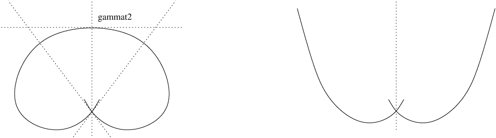
Refer to caption
Figure 14: A reverse loop and its image under a projective transformation.

If γ\gamma has a single self-tangency (t0,t1)(t_{0},t_{1}) of order 33 start by perturbing a neighborhood of the self-tangency in such a way as to create exactly one transversal double point. Any direct loop of γ^\hat{\gamma} except for (t0,t1)(t_{0},t_{1}) (if it is simple) yields a direct loop of γ\gamma. Thus, the only situation where γ\gamma does not have a direct loop is if (t0,t1)(t_{0},t_{1}) is the unique direct loop of γ^\hat{\gamma}; this completes the proof.     ■\blacksquare

Two loops (t0,t1)(t_{0},t_{1}) and (t~0,t~1)(\tilde{t}_{0},\tilde{t}_{1}) are disjoint if the intervals [t0,t1]⊂𝕊1[t_{0},t_{1}]\subset{\mathbb{S}}^{1} and [t~0,t~1]⊂𝕊1[\tilde{t}_{0},\tilde{t}_{1}]\subset{\mathbb{S}}^{1} are disjoint. Notice that this does not mean that the images of the intervals under γ\gamma are disjoint.

A curve γ∈ℒI(1)∖(ℒ−1,c∪𝒯0∪ℰ)\gamma\in{\cal L}^{(1)}_{I}\smallsetminus({\cal L}_{-1,c}\cup{\cal T}_{0}\cup{\cal E}) is a pseudo-egg if it belongs to the connected component of one of the curves in the infinite family indicated in Figure 15. More precisely, γ\gamma admits two non disjoint direct loops (t0,t1)(t_{0},t_{1}) and (t2,t3)(t_{2},t_{3}), t0<t2<t1<t3<t0+1t_{0}<t_{2}<t_{1}<t_{3}<t_{0}+1, and the restriction of γ\gamma to [t3,t0+1][t_{3},t_{0}+1] is injective. Let ℰ+{\cal E}^{+} be the set of eggs and pseudo-eggs.

Refer to caption
Figure 15: Pseudo-eggs
Lemma 6.3

Let KK be a compact manifold and f:K→ℒI∖(ℒ−1,c∪𝒯0∪ℰ)f:K\to{\cal L}_{I}\smallsetminus({\cal L}_{-1,c}\cup{\cal T}_{0}\cup{\cal E}) a continuous map. Then ff is homotopic in ℒI∖(ℒ−1,c∪𝒯0∪ℰ){\cal L}_{I}\smallsetminus({\cal L}_{-1,c}\cup{\cal T}_{0}\cup{\cal E}) to some map f^:K→ℒI∖(ℒ−1,c∪𝒯0∪ℰ+)\hat{f}:K\to{\cal L}_{I}\smallsetminus({\cal L}_{-1,c}\cup{\cal T}_{0}\cup{\cal E}^{+}).

Proof: Consider the innermost loop in the spiral and pull it (using Δ♯\Delta^{\sharp}) as in Figure 16: this will either do a Reidemeister move of type III or of type II, in either case destroying the pseudo-egg.     ■\blacksquare

Refer to caption
Figure 16: How to get rid of pseudo-eggs
Lemma 6.4

Consider a curve γ∈ℒI(1)∖(ℒ−1,c∪𝒯0∪ℰ+)\gamma\in{\cal L}^{(1)}_{I}\smallsetminus({\cal L}_{-1,c}\cup{\cal T}_{0}\cup{\cal E}^{+}). For every direct loop (t0,t1)(t_{0},t_{1}) of γ\gamma there is a disjoint direct loop (t2,t3)(t_{2},t_{3}). For every reverse loop (t0,t1)(t_{0},t_{1}) of γ\gamma there is a disjoint (reverse or direct) loop (t2,t3)(t_{2},t_{3}). Furthermore, given two non-disjoint direct loops (t0,t1)(t_{0},t_{1}) and (t2,t3)(t_{2},t_{3}), γ\gamma admits a loop (t4,t5)(t_{4},t_{5}) which is disjoint from both (t0,t1)(t_{0},t_{1}) and (t2,t3)(t_{2},t_{3}).

The second part does not always hold if (t0,t1)(t_{0},t_{1}) and (t2,t3)(t_{2},t_{3}) are reverse: see Figure 17, (a). In the last claim, the new loop in case (a) may be reverse: see Figure 17, (b).

Refer to caption
Figure 17: Non-disjoint loops (t0,t1)(t_{0},t_{1}) and (t2,t3)(t_{2},t_{3}).

Proof: Assume γ∈ℒI(1)\gamma\in{\cal L}^{(1)}_{I} so that every self-intersection is transversal. Let (t0,t1)(t_{0},t_{1}) be a loop. It (t1,t0+1)(t_{1},t_{0}+1) is a loop then γ\gamma is a star. Otherwise, take t∗=t1+ϵt_{\ast}=t_{1}+\epsilon (ϵ>0\epsilon>0, ϵ\epsilon small). As in Lemma 6.2, let t3t_{3} be the smallest t>t∗t>t_{\ast} such that γ|[t∗,t]\gamma|_{[t_{\ast},t]} is not injective and let t2∈[t∗,t3)t_{2}\in[t_{\ast},t_{3}) be such that γ⁡(t2)=γ⁡(t3)\gamma(t_{2})=\gamma(t_{3}), so that (t2,t3)(t_{2},t_{3}) is a loop. Since (t1,t0+1)(t_{1},t_{0}+1) is not a loop, t3<t0+1t_{3}<t_{0}+1 and (t2,t3)(t_{2},t_{3}) is disjoint from (t0,t1)(t_{0},t_{1}), as required.

Let (t0,t1)(t_{0},t_{1}), (t2,t3)(t_{2},t_{3}) be two non-disjoint loops. The case t0=t2t_{0}=t_{2}, t1=t3t_{1}=t_{3} was discussed in the previous paragraph; t2=t1t_{2}=t_{1}, t3=t0+1t_{3}=t_{0}+1 implies that γ\gamma is a star. We may therefore assume t0<t2<t1<t3<t0+1t_{0}<t_{2}<t_{1}<t_{3}<t_{0}+1, as in Figure 18.

Refer to caption
Figure 18: Two non-disjoint loops.

Notice that (𝔉γ​(t0))−1​𝔉γ​(t3)∈𝒥2({\mathfrak{F}}_{\gamma}(t_{0}))^{-1}{\mathfrak{F}}_{\gamma}(t_{3})\in{\cal J}_{2}. If the restriction γ|[t3,t0+1]\gamma|_{[t_{3},t_{0}+1]} is convex then γ\gamma is a star (Figure 18 (b)). If the restriction is injective but not convex then γ\gamma is either an egg or a pseudo-egg (Figure 18 (c)). Finally, if the above restriction is not injective then a new loop disjoint from (t0,t1)(t_{0},t_{1}) and (t2,t3)(t_{2},t_{3}) exists (Figure 18 (d)).     ■\blacksquare

7 Proof of the main results

Lemma 7.1

The connected components of ℒI∖(ℒ−1,c∪𝒯0){\cal L}_{I}\smallsetminus({\cal L}_{-1,c}\cup{\cal T}_{0}) are simply connected.

Proof: Let f:𝕊1→ℒI∖(ℒ−1,c∪𝒯0)f:{\mathbb{S}}^{1}\to{\cal L}_{I}\smallsetminus({\cal L}_{-1,c}\cup{\cal T}_{0}) be a continuous map. We prove that ff is homotopic to a point. By Lemma 6.1 and transversality we may assume f:𝕊1→ℒI(2)∖(ℒ−1,c∪𝒯0∪ℰ)f:{\mathbb{S}}^{1}\to{\cal L}^{(2)}_{I}\smallsetminus({\cal L}_{-1,c}\cup{\cal T}_{0}\cup{\cal E}) and that f⁡(p)∈ℒI(1)f(p)\in{\cal L}^{(1)}_{I} except for finitely many points p1,…,pM∈𝕊1p_{1},\ldots,p_{M}\in{\mathbb{S}}^{1}. In case M≤2M\leq 2 add a few points to the list to guarantee M≥3M\geq 3. Reparametrize so that pk=kM∈𝕊1p_{k}=\frac{k}{M}\in{\mathbb{S}}^{1}. By Lemma 6.2, for every p∈𝕊1p\in{\mathbb{S}}^{1} the curve f⁡(p)f(p) has a direct loop. Let Vk=(k−1M,k+1M)V_{k}=(\frac{k-1}{M},\frac{k+1}{M}) and use a direct loop of f⁡(kM)f(\frac{k}{M}) to define t0,k,t1,k:Vk→𝕊1t_{0,k},t_{1,k}:V_{k}\to{\mathbb{S}}^{1}. This is an open cover, but the loops are probably not disjoint.

Let Uk=(3​k−13​M,3​k+13​M)U_{k}=(\frac{3k-1}{3M},\frac{3k+1}{3M}). Let p⋆=2​k+12​Mp_{\star}=\frac{2k+1}{2M}, γ⋆=f⁡(p⋆)∈ℒI(1)\gamma_{\star}=f(p_{\star})\in{\cal L}^{(1)}_{I}, t0=t0,k​(p⋆)t_{0}=t_{0,k}(p_{\star}), t1=t1,k​(p⋆)t_{1}=t_{1,k}(p_{\star}), t2=t0,k+1​(p⋆)t_{2}=t_{0,k+1}(p_{\star}) and t3=t1,k+1​(p⋆)t_{3}=t_{1,k+1}(p_{\star}). If the loops (t0,t1)(t_{0},t_{1}) and (t2,t3)(t_{2},t_{3}) of γ⋆\gamma_{\star} are equal or disjoint, set Uk+1/2=(kM,k+1M)U_{k+1/2}=(\frac{k}{M},\frac{k+1}{M}) and t∗,k+1/2​(p)=t∗,k​(p)t_{\ast,k+1/2}(p)=t_{\ast,k}(p). If these two loops are not disjoint, use Lemma 6.4 to obtain two loops (t4,t5)(t_{4},t_{5}) and (t6,t7)(t_{6},t_{7}) of γ⋆\gamma_{\star} such that:

  1. 1.

    (t4,t5)(t_{4},t_{5}) is disjoint from (t0,t1)(t_{0},t_{1});

  2. 2.

    (t6,t7)(t_{6},t_{7}) is disjoint from (t2,t3)(t_{2},t_{3});

  3. 3.

    (t4,t5)(t_{4},t_{5}) and (t6,t7)(t_{6},t_{7}) are either equal or disjoint.

Set Uk+1/3=(kM,3​k+23​M)U_{k+1/3}=(\frac{k}{M},\frac{3k+2}{3M}) and Uk+2/3=(3​k+13​M,k+1M)U_{k+2/3}=(\frac{3k+1}{3M},\frac{k+1}{M}); use (t4,t5)(t_{4},t_{5}) and (t6,t7)(t_{6},t_{7}) to define (t0,k+1/3,t1,k+1/3)(t_{0,k+1/3},t_{1,k+1/3}) and (t0,k+2/3,t1,k+2/3)(t_{0,k+2/3},t_{1,k+2/3}), respectively. Thus, ff admits a cover by disjoint loops. From Lemma 4.5, ff is homotopic to ν2∗f\nu_{2}\ast f.

On the other hand, each connected component of ℐI{\cal I}_{I} is simply connected and therefore ff is homotopic to a point in ℐI{\cal I}_{I}. By Proposition 2.1 ff is homotopic to a point in ℒI{\cal L}_{I}. The homotopy can be constructed as follows: consider an extension f^:𝔻2→ℐI\hat{f}:{\mathbb{D}}^{2}\to{\cal I}_{I} of ff; use Δ♯\Delta^{\sharp} to pass from ff to FN∘fF_{N}\circ f and complete the homotopy with FN∘f^F_{N}\circ\hat{f}. For sufficiently large NN, this homotopy remains in ℒI∖(ℒ−1,c∪𝒯0){\cal L}_{I}\smallsetminus({\cal L}_{-1,c}\cup{\cal T}_{0}).     ■\blacksquare

Theorem 2

Each connected component of ℒI{\cal L}_{I} is simply connected.

Proof: It is well known that ℒ−1,c{\cal L}_{-1,c} is contractible. Since 𝒯0⊂ℒ+1{\cal T}_{0}\subset{\cal L}_{+1}, we just proved that in Lemma 7.1 that ℒ−1,n{\cal L}_{-1,n} is also simply connected. Finally, we use Seifert-Van Kampen to compute π1​(ℒ+1)\pi_{1}({\cal L}_{+1}). Let A=ℒ+1∖𝒯0A={\cal L}_{+1}\smallsetminus{\cal T}_{0} and fatten 𝒯0{\cal T}_{0} a bit to obtain an open set BB: since 𝒯0{\cal T}_{0} is contractible and 𝒯1=∂𝒯0{\cal T}_{1}=\partial{\cal T}_{0} is a connected submanifold of codimension 11, BB is simply connected and A∩BA\cap B is connected. Thus, ℒ+1=A∪B{\cal L}_{+1}=A\cup B is also simply connected.     ■\blacksquare

Lemma 7.2

Let γ∈ℒI(1)∖(ℒ−1,c∪𝒯0∪ℰ+)\gamma\in{\cal L}^{(1)}_{I}\smallsetminus({\cal L}_{-1,c}\cup{\cal T}_{0}\cup{\cal E}^{+}). Let f:𝔻2→ℒI∖𝒯0f:{\mathbb{D}}^{2}\to{\cal L}_{I}\smallsetminus{\cal T}_{0} be the function constant equal to γ\gamma. Consider a disjoint cover by loops 𝒞{\cal C} of f|𝕊1f|_{{\mathbb{S}}^{1}} without two consecutive reverse loops. Then there exists f~:𝔻2→ℒI∖𝒯0\tilde{f}:{\mathbb{D}}^{2}\to{\cal L}_{I}\smallsetminus{\cal T}_{0} homotopic to ff with fixed boundary and an extension 𝒞~\tilde{\cal C} of 𝒞{\cal C} to a disjoint cover by loops of f~\tilde{f}.

Proof: Without loss of generality the open sets in the cover are intervals. If two neighboring intervals have identical loops, fuse them; may therefore assume without loss of generality that 𝕊1{\mathbb{S}}^{1} is covered by a cycle of loops, where two adjacent loops are disjoint and no two adjacent loops are both reverse. More: if two non-adjacent intervals use the same loop, the corresponding open set can be enlarged to cross the disk (Figure 19,(a)). We may therefore assume all loops to be distinct.

Refer to caption
Figure 19: Long cycles can be decomposed into short ones.

If the cycle 77 or more loops, it can be decomposed into cycles of size 66 or less. Indeed, consider a cycle of length n>6n>6; let ℓ0\ell_{0} be a direct loop in the cycle and let ℓ1,ℓ2,ℓ3,ℓ4\ell_{1},\ell_{2},\ell_{3},\ell_{4} be its neighbors (numbered clockwise). Let i=3i=3 or 44 such that ℓi\ell_{i} is direct. If ℓ0\ell_{0} and ℓi\ell_{i} are disjoint, extend the open sets V0V_{0} and ViV_{i} to intersect in the center, thus subdividing the original cycle into one of length i+1i+1 and another of length n−i+1n-i+1 (Figure 19,(b)). If ℓ0\ell_{0} and ℓi\ell_{i} are not disjoint, use Lemma 6.4 to obtain a loop ℓ~\tilde{\ell} disjoint from both: introduce an open set V~\tilde{V} with associated loop ℓ~\tilde{\ell} in the middle of the disk, intersecting V0V_{0} and ViV_{i} only among the originally defined loops. This subdivides the original cycle into two cycles of lengths i+2i+2 and n−i+2n-i+2 (Figure 19,(c)).

Cycles of 22 or 33 loops have all loops disjoint and therefore admit a disjoint cover as they are, no homotopy needed. We are left with considering cycles of length 44, 55 or 66.

From now on we argue by contradiction, searching for the shortest counterexample. If two non-adjacent loops are disjoint, not both reverse, construction (b) in Figure 19 can be applied, decomposing our cycle into two shorter ones. We may therefore assume that non-adjacent loops not both reverse are not disjoint.

We first consider the case n=6n=6. If two opposite loops ℓi\ell_{i} and ℓi+3\ell_{i+3} are both direct then the construction in Figure 19 (b) or (c) can be applied, decomposing our cycle. We may therefore assume that ℓi\ell_{i} is direct for ii even and reverse for ii odd. Consider the intervals Ii=[t0,i,t1,i]⊂𝕊1I_{i}=[t_{0,i},t_{1,i}]\subset{\mathbb{S}}^{1}: I0I_{0}, I2I_{2} and I4I_{4} are pairwise neither disjoint not nested (one contained in the other). There are, up to reparametrization and permutation, only two possibilities: I0=[0,3/6]I_{0}=[0,3/6], I2=[1/6,4/6]I_{2}=[1/6,4/6], I4=[−1/6,2/6]I_{4}=[-1/6,2/6] or I0=[0,3/6]I_{0}=[0,3/6], I2=[2/6,5/6]I_{2}=[2/6,5/6], I4=[−2/6,1/6]I_{4}=[-2/6,1/6]. In either case, I3I_{3} must be disjoint from both I2I_{2} and I4I_{4} and neither disjoint nor nested with I0I_{0}, a contradiction.

Consider now the case n=5n=5, with loops ℓ0,…,ℓ4\ell_{0},\ldots,\ell_{4}. We may assume without loss of generality that ℓ0\ell_{0}, ℓ2\ell_{2} and ℓ3\ell_{3} are direct loops, ℓ2\ell_{2} and ℓ3\ell_{3} disjoint but ℓ0\ell_{0} not disjoint from either. We may again assume that I0=[1/10,4/10]I_{0}=[1/10,4/10], I2=[0,2/10]I_{2}=[0,2/10], I3=[3/10,5/10]I_{3}=[3/10,5/10] and that the image of [0,5/10][0,5/10] under γ\gamma is as in Figure 20. Pull the loop ℓ0\ell_{0} (or, in other words, apply Δ♯​(s,γ,1/10−ϵ,4/10+ϵ)\Delta^{\sharp}(s,\gamma,1/10-\epsilon,4/10+\epsilon)) in the center of the disk 𝔻2{\mathbb{D}}^{2} to define f~\tilde{f}. The loops ℓ0,ℓ2,ℓ3\ell_{0},\ell_{2},\ell_{3} survive in 𝔻2{\mathbb{D}}^{2} and near the center of 𝔻2{\mathbb{D}}^{2}, ℓ0\ell_{0} becomes disjoint from ℓ2,ℓ3\ell_{2},\ell_{3}. The loops ℓ1\ell_{1} and ℓ4\ell_{4} were not affected and remain disjoint from ℓ0\ell_{0}. We therefore have the disjoint cover in Figure 20.

Refer to caption
Figure 20: The case n=5n=5

Finally, for n=4n=4, we may assume that ℓ0\ell_{0} and ℓ2\ell_{2} are direct. As in Figure 21, pulling either ℓ0\ell_{0} or ℓ2\ell_{2} (or both) makes them disjoint. The disjoint cover in Figure 21 completes the proof.     ■\blacksquare

Refer to caption
Figure 21: The case n=4n=4
Lemma 7.3

Every continuous map f:𝕊2→ℒI∖(ℒ−1,c∪𝒯0)f:{\mathbb{S}}^{2}\to{\cal L}_{I}\smallsetminus({\cal L}_{-1,c}\cup{\cal T}_{0}) is homotopic to ν2∗f\nu_{2}\ast f.

Proof: It is enough to prove that ff is homotopic to some f~\tilde{f} which admits a disjoint cover. By Lemmas 6.1, 6.3 and transversality we may assume f:𝕊1→ℒI(3)∖(ℒ−1,c∪𝒯0∪ℰ+)f:{\mathbb{S}}^{1}\to{\cal L}^{(3)}_{I}\smallsetminus({\cal L}_{-1,c}\cup{\cal T}_{0}\cup{\cal E}^{+}). Again by transversality, we may assume that there exists a finite triangulation of 𝕊2{\mathbb{S}}^{2} such that if f⁡(p)∉ℒI(2)f(p)\notin{\cal L}^{(2)}_{I} then pp is a vertex of the triangulation and if f⁡(p)∉ℒI(1)f(p)\notin{\cal L}^{(1)}_{I} then pp belongs to an edge. By Lemma 6.2, there exist open neighborhoods ViV_{i} of the vertices and direct loops t0,i,t1,i:Vi→𝕊1t_{0,i},t_{1,i}:V_{i}\to{\mathbb{S}}^{1}. As in the proof of Lemma 7.1, there exists a disjoint cover of each edge by loops without two consecutive reverse loops. It remain to fill in the faces: this is precisely what Lemma 7.2 does.     ■\blacksquare

Theorem 3

We have π2​(ℒ+1)=ℤ2\pi_{2}({\cal L}_{+1})={\mathbb{Z}}^{2}, π2​(ℒ−1,n)=ℤ\pi_{2}({\cal L}_{-1,n})={\mathbb{Z}}, H2​(ℒ+1,ℤ)=ℤ2H^{2}({\cal L}_{+1};{\mathbb{Z}})={\mathbb{Z}}^{2} and H2​(ℒ−1,n,ℤ)=ℤH^{2}({\cal L}_{-1,n};{\mathbb{Z}})={\mathbb{Z}}.

Proof: By the previous lemma, f:𝕊2→ℒ−1,nf:{\mathbb{S}}^{2}\to{\cal L}_{-1,n} is homotopic to a point in ℒ−1,n{\cal L}_{-1,n} if and only if it is homotopic to a point in ℐ−1,n{\cal I}_{-1,n}. In other words, the inclusion ℒ−1,n⊂ℐ−1{\cal L}_{-1,n}\subset{\cal I}_{-1} induces an isomorphism between π2​(ℒ−1,n)\pi_{2}({\cal L}_{-1,n}) and π2​(ℐ−1)=ℤ\pi_{2}({\cal I}_{-1})={\mathbb{Z}}. By Hurewicz theorem, inclusion also yields an isomorphism between H2​(ℒ−1,n,ℤ)H^{2}({\cal L}_{-1,n};{\mathbb{Z}}) and H2​(ℐ−1,ℤ)=ℤH^{2}({\cal I}_{-1};{\mathbb{Z}})={\mathbb{Z}}. In other words, H2​(ℒ−1,n,ℤ)H^{2}({\cal L}_{-1,n};{\mathbb{Z}}) is generated by 𝐱{\bf x}.

Similarly, H2​(ℒ+1∖𝒯0,ℤ)H^{2}({\cal L}_{+1}\smallsetminus{\cal T}_{0};{\mathbb{Z}}) is generated by 𝐱{\bf x}. Use the normal bundle to 𝒯1{\cal T}_{1} to define open sets AA and BB, 𝒯0⊂A{\cal T}_{0}\subset A, ℒ+1∖𝒯0⊂B{\cal L}_{+1}\smallsetminus{\cal T}_{0}\subset B such that the above inclusions and 𝒯1⊂A∩B{\cal T}_{1}\subset A\cap B are homotopy equivalences. Write the Mayer-Vietoris sequence (coefficients in ℤ{\mathbb{Z}}):

H1​(A)⊕H1​(B)→H1​(A∩B)→H2​(A∪B)→H2​(A)⊕H2​(B)→H2​(A∩B)H^{1}(A)\oplus H^{1}(B)\to H^{1}(A\cap B)\to H^{2}(A\cup B)\to H^{2}(A)\oplus H^{2}(B)\to H^{2}(A\cap B)

We know that H1​(A)=H1​(B)=0H^{1}(A)=H^{1}(B)=0, H1​(A∩B)=ℤH^{1}(A\cap B)={\mathbb{Z}}, H2​(A)=0H^{2}(A)=0, H2​(B)=ℤH^{2}(B)={\mathbb{Z}}, H2​(A∩B)=0H^{2}(A\cap B)=0. Thus H2​(A∪B)=ℤ2H^{2}(A\cup B)={\mathbb{Z}}^{2}. In the proof of Lemma 5.1 we saw a geometric description of the universal cover and therefore of the generator of H1​(A∩B)H^{1}(A\cap B): appying the map H1​(A∩B)→H2​(A∪B)H^{1}(A\cap B)\to H^{2}(A\cup B) to this generator obtains 𝐟2∈H2​(ℒ+1){\bf f}_{2}\in H^{2}({\cal L}_{+1}), the intersection number with ℱ2⊂𝒯1{\cal F}_{2}\subset{\cal T}_{1}. Thus, H2​(ℒ+1CLOSEH^{2}({\cal L}_{+1} is generated by 𝐱{\bf x} and 𝐟2{\bf f}_{2}. Again by Hurewicz theorem, π2​(ℒ+1)=ℤ2\pi_{2}({\cal L}_{+1})={\mathbb{Z}}^{2} is generated by 𝐠2{\bf g}_{2} and ν2∗𝐠2\nu_{2}\ast{\bf g}_{2}.     ■\blacksquare

8 Final remarks

It may be possible to carry further methods used in this paper to compute H∗​(ℒI)H^{\ast}({\cal L}_{I}), but the kind of case-by-case analysis in Section 6 would have to be replaced by something less accidental. We hope to do this in [3] to prove that the classes 𝐱n{\bf x}^{n} and 𝐟2​n{\bf f}_{2n} are generators of H∗​(ℒ±1)H^{\ast}({\cal L}_{\pm 1}) and that ℒ+1{\cal L}_{+1} and ℒ−1,n{\cal L}_{-1,n} have the homotopy type of Ω​𝕊3∨𝕊2∨𝕊6∨𝕊10∨⋯\Omega{\mathbb{S}}^{3}\vee{\mathbb{S}}^{2}\vee{\mathbb{S}}^{6}\vee{\mathbb{S}}^{10}\vee\cdots and Ω​𝕊3∨𝕊4∨𝕊8∨𝕊12∨⋯\Omega{\mathbb{S}}^{3}\vee{\mathbb{S}}^{4}\vee{\mathbb{S}}^{8}\vee{\mathbb{S}}^{12}\vee\cdots, respectively.

References

  • [1] Burde, G. and Zieschang, H., Knots, Walter de Gruyter, Berlin, 1985.
  • [2] Little, J. A., Nondegenerate homotopies of curves on the unit 2-sphere, J. Differential Geometry, 4, 339-348, 1970.
  • [3] Saldanha, N., The homotopy type of spaces of locally convex curves in the sphere, in preparation.
  • [4] Saldanha, N., The cohomology of spaces of locally convex curves in the sphere — I, preprint, arXiv:0905.2111v1.
  • [5] Saldanha, N. and Shapiro, B., Spaces of locally convex curves in SnS^{n} and combinatorics of the group Bn+1+B^{+}_{n+1}, Journal of Singularities, 4, 1-22, 2012.
  • [6] Shapiro, B. and Khesin, B., Homotopy classification of nondegenerate quasiperiodic curves on the 22-sphere, Publ. Inst. Math. (Beograd) 66(80), 127-156, 1999.
  • [7] Shapiro, M., Topology of the space of nondegenerate curves, Math. USSR, 57, 106-126, 1993.

Nicolau C. Saldanha, PUC-Rio

saldanha@puc-rio.br; http://www.mat.puc-rio.br/∼\simnicolau/

Departamento de Matemática, PUC-Rio

R. Marquês de S. Vicente 225, Rio de Janeiro, RJ 22453-900, Brazil