The homotopy and cohomology of spaces
of locally convex curves in the sphere — I

A curve $\gamma:[0,1]\to{\mathbb{S}}^{2}$ is called locally convex if its geodesic curvature is always positive, or, equivalently, if $\det(\gamma(t),\gamma^{\prime}(t),\gamma^{\prime\prime}(t))>0$ for all $t$. Let ${\cal L}_{I}$ be the space of all locally convex curves $\gamma$ with $\gamma(0)=\gamma(1)=e_{1}$ and $\gamma^{\prime}(0)=\gamma^{\prime}(1)=e_{2}$. The topology in this space of curves will be given by the Sobolev metric $H^{2}$: this has the minor technical advantages of making ${\cal L}_{I}$ a Hilbert manifold and of allowing for jump discontinuities in $\gamma^{\prime\prime}$ in the constructions. The choice of metric actually makes very little difference: since it is easy to uniformly smoothen out a curve while keeping its geodesic curvature positive we might just as well work with the $C^{\infty}$ topology, or with $C^{k}$ for some $k\geq 2$.

J. A. Little [7] showed that ${\cal L}_{I}$ has three connected components ${\cal L}_{-1,c}$, ${\cal L}_{+1}$, ${\cal L}_{-1,n}$: we call these the Little spaces. Figure 1 shows examples of curves in ${\cal L}_{-1,c}$, ${\cal L}_{+1}$ and ${\cal L}_{-1,n}$, respectively. The connected component ${\cal L}_{-1,c}$ consists of the simple curves in ${\cal L}_{I}$: the space ${\cal L}_{-1,c}$ is known to be contractible ([15], Lemma 5). The topology of these and related spaces has been discussed, among others, by B. Shapiro, M. Shapiro and Khesin ([14], [13]) but the topology of the Little spaces is still not well understood. This series of papers is to present new results concerning the homotopy and cohomology of the Little spaces. A more ambitious aim would be to determine the homotopy type of these spaces (which we hope to accomplish in [9]).

Let ${\cal I}_{I}\supset{\cal L}_{I}$ be the space of immersions $\gamma:[0,1]\to{\mathbb{S}}^{2}$, $\gamma^{\prime}(t)\neq 0$, $\gamma(0)=\gamma(1)=e_{1}$, $\gamma^{\prime}(0)=\gamma^{\prime}(1)=e_{2}$. For each $\gamma\in{\cal I}_{I}$, consider its Frenet frame ${\mathfrak{F}}_{\gamma}:[0,1]\to SO(3)$ defined by

$$\begin{pmatrix}\gamma(t)&\gamma^{\prime}(t)&\gamma^{\prime\prime}(t)\end{pmatrix}={\mathfrak{F}}_{\gamma}(t)R(t),$$

$R(t)$ being an upper triangular matrix with positive diagonal (the left hand side is the $3\times 3$ matrix with columns $\gamma(t)$, $\gamma^{\prime}(t)$ and $\gamma^{\prime\prime}(t)$). The universal (double) cover of $SO(3)$ is ${\mathbb{S}}^{3}\subset{\mathbb{H}}$, the group of quaternions of absolute value $1$; let $\Pi:{\mathbb{S}}^{3}\to SO(3)$ be the canonical projection. The curve ${\mathfrak{F}}_{\gamma}$ can be lifted to define $\tilde{\mathfrak{F}}_{\gamma}:[0,1]\to{\mathbb{S}}^{3}$ with $\tilde{\mathfrak{F}}_{\gamma}(0)=1$, $\Pi\circ\tilde{\mathfrak{F}}_{\gamma}={\mathfrak{F}}_{\gamma}$. The value of $\tilde{\mathfrak{F}}_{\gamma}(1)$ defines the two connected components ${\cal I}_{\pm 1}$ of ${\cal I}_{I}$: $\gamma\in{\cal I}_{+1}$ if and only if $\tilde{\mathfrak{F}}_{\gamma}(1)=1$. Notice that if $\gamma$ is a simple curve in ${\cal I}_{I}$ then $\tilde{\mathfrak{F}}_{\gamma}(1)=-1$ and therefore $\gamma\in{\cal I}_{-1}$. We have ${\cal L}_{+1}={\cal I}_{+1}\cap{\cal L}_{I}$ and ${\cal L}_{-1}={\cal L}_{-1.c}\sqcup{\cal L}_{-1,n}={\cal I}_{-1}\cap{\cal L}_{I}$.

Let $\Omega{\mathbb{S}}^{3}$ (resp. $\Omega_{-}{\mathbb{S}}^{3}$) be the set of continuous curves $\alpha:[0,1]\to{\mathbb{S}}^{3}$, $\alpha(0)=\alpha(1)=1$ (resp. $\alpha(0)=1$, $\alpha(1)=-1$). These two spaces are easily seen to be homeomorphic and shall from now on be identified; $\Omega{\mathbb{S}}^{3}$ is a well understood space: we have $H^{\ast}(\Omega{\mathbb{S}}^{3},{\mathbb{R}})={\mathbb{R}}[{\mathbf{x}}]$ where ${\mathbf{x}}\in H^{2}$ satisfies ${\mathbf{x}}^{n}\neq 0$ for all positive $n$ (see, for instance, [1]). The previous paragraph defines maps $\tilde{\mathfrak{F}}:{\cal I}_{\pm 1}\to\Omega{\mathbb{S}}^{3}$. It is a well-known fact that these two maps are homotopy equivalences; this follows from the Hirsch-Smale Theorem ([8], [6], [16]). As we shall see, the inclusions $i:{\cal L}_{\pm 1}\to{\cal I}_{\pm 1}$ are not homotopy equivalences.

The maps $i:{\cal L}_{\pm 1}\to{\cal I}_{\pm 1}$ therefore induce surjective maps $\pi_{k}({\cal L}_{\pm 1})\to\pi_{k}({\cal I}_{\pm 1})$. In fact, since ${\cal L}_{\pm 1}$ and ${\cal I}_{\pm 1}$ have the homotopy type of CW complexes with finitely many cells per dimension, the inclusions are homotopically surjective but we skip the details.

In particular, ${\cal L}_{\pm 1}$ is not homotopically equivalent to a finite CW-complex. Theorem 2 in [11] is a similar result for arbitrary dimension. From Theorem 1 we write ${\mathbb{R}}[{\mathbf{x}}]\subseteq H^{\ast}({\cal L}_{\pm 1};{\mathbb{R}})$. The main result of this paper implies that ${\mathbb{R}}[{\mathbf{x}}]$ has infinite codimension as a subspace of $H^{\ast}({\cal L}_{\pm 1})$.

Let ${\cal L}$ be the contractible space of all locally convex curves $\gamma$ with $\gamma(0)=e_{1}$ and $\gamma^{\prime}(0)=e_{2}$ and define $\phi:{\cal L}\to{\mathbb{S}}^{3}$ by $\phi(\gamma)=\tilde{\mathfrak{F}}_{\gamma}(1)$ where $\tilde{\mathfrak{F}}_{\gamma}:[0,1]\to{\mathbb{S}}^{3}$ is defined via Frenet frames as above. It is natural to conjecture that $\phi:{\cal L}\to{\mathbb{S}}^{3}$ is somehow similar to a fibration.

This is not the case: we prove that the map $\phi$ does not satisfy the homotopy lifting property. Let $X=[0,1]^{2}$. There exist maps ${\mathbf{h}}:X\times[0,1]\to{\mathbb{S}}^{3}$ and $\tilde{\mathbf{h}}_{0}:X\times\{0\}\to{\cal L}$ such that $\phi\circ\tilde{\mathbf{h}}_{0}={\mathbf{h}}|_{X\times\{0\}}$ and there exists no map $\tilde{\mathbf{h}}:X\times[0,1]\to{\cal L}$ with $\phi\circ\tilde{\mathbf{h}}={\mathbf{h}}$. The maps ${\mathbf{h}}$ and $\tilde{\mathbf{h}}_{0}$ will be constructed explicitly in Section 6.

A curve $\gamma\in{\cal L}_{(-1)^{(k+1)}}$ is a flower of $2k+1$ petals if there exist $0=t_{0}<t_{1}<t_{2}<\cdots<t_{2k}<t_{2k+1}=1$ and $0=\theta_{0}<\theta_{1}<\theta_{2}<\cdots<\theta_{2k}<\theta_{2k+1}=\theta_{M}$ such that:

1. 1.

   $\gamma(t_{1})=\gamma(t_{2})=\cdots=\gamma(t_{2k})=e_{1}$;

2. 2.

   the only self-intersections of the curve $\gamma$ are of the form $\gamma(t_{i})=\gamma(t_{j})$;

3. 3.

   the argument of $(x_{i,2},x_{i,3})$ is $\theta_{i}$, where $(0,x_{i,2},x_{i,3})=(-1)^{i}\gamma^{\prime}(t_{i})$.

As a somewhat degenerate case, a flower of $1$ petal is a simple locally convex curve. Figure 2 shows examples of flowers.

For $k>0$, let ${\cal F}_{2k}\subset{\cal L}_{(-1)^{(k+1)}}$ be the set of flowers of $2k+1$ petals. As we shall see in Lemma 4.1, the set ${\cal F}_{2k}$ is closed and a submanifold of codimension $2k$. Furthermore, the normal bundle to ${\cal F}_{2k}$ in ${\cal L}_{(-1)^{(k+1)}}$ is trivial. Thus, intersection with ${\cal F}_{2k}$ defines an element ${\mathbf{f}}_{2k}\in H^{2k}({\cal L}_{(-1)^{(k+1)}})$ with $({\mathbf{f}}_{2k})^{2}=0$.

We shall construct maps ${\mathbf{g}}_{2k}:{\mathbb{S}}^{2k}\to{\cal L}_{(-1)^{(k+1)}}$ which are homotopic to a constant in ${\cal I}_{(-1)^{(k+1)}}$ but which satisfy ${\mathbf{f}}_{2k}{\mathbf{g}}_{2k}=1$, thus proving that both ${\mathbf{f}}_{2k}\in H^{2k}({\cal L}_{\pm 1})$ and ${\mathbf{g}}_{2k}\in\pi_{2k}({\cal L}_{\pm 1})$ are nontrivial. This establishes our main result.

Notice that ${\cal L}_{per}$, the set of all $1$-periodic locally convex curves $\tilde{\gamma}:{\mathbb{R}}\to{\mathbb{S}}^{2}$, is homeomorphic to $SO(3)\times{\cal L}_{I}$: define $\Psi:{\cal L}_{per}\to SO(3)\times{\cal L}_{I}$ by $\Psi(\tilde{\gamma})=({\mathfrak{F}}_{\tilde{\gamma}}(0),({\mathfrak{F}}_{\tilde{\gamma}}(0))^{-1}\tilde{\gamma}|_{[0,1]})$. We usually prefer to work in ${\cal L}_{I}$ but sometimes move to ${\cal L}_{per}$.

In Section 2, we give a brief sketch of Little’s Theorem and present the concept of convex curves. Section 3 is dedicated to Theorem 1. In Section 4, we prove the basic facts about the set of flowers. Section 5 contains the construction of the map ${\mathbf{g}}_{2}:{\mathbb{S}}^{2}\to{\cal L}_{+1}$ and the proof of Theorem 2 for $k=1$. The construction of the maps ${\mathbf{h}}:X\times[0,1]\to{\mathbb{S}}^{3}$ and $\tilde{\mathbf{h}}_{0}:X\times\{0\}\to{\cal L}$ are presented in Section 6. Finally, in Section 7, we construct the maps ${\mathbf{g}}_{2k}:{\mathbb{S}}^{2k}\to{\cal L}_{(-1)^{(k+1)}}$ and prove Theorem 2 for $k>1$. Section 8 contains a few final remarks.

In the second paper of this series ([10]) we prove that the connected components of ${\cal L}_{I}$ are simply connected and compute the groups $H^{2}({\cal L}_{\pm 1};{\mathbb{Z}})$.

This work was motivated by an attempt to extend to ordinary differential equations of order $3$ some of our results with Dan Burghelea and Carlos Tomei ([2], [3]). Consider the differential equation of order 3:

$$u^{\prime\prime\prime}(t)+h_{1}(t)u^{\prime}(t)+h_{0}(t)u(t)=0,\quad t\in[0,1];$$

the set of pairs of potentials $(h_{0},h_{1})$ for which the equation admits 3 linearly independent periodic solutions is homotopically equivalent to ${\cal L}_{I}$ ([12]). The motivation of B. Shapiro and M. Shapiro for studying these spaces is similar.

The author would like to thank Dan Burghelea and Boris Shapiro for helpful conversations. The author acknowledges the hospitality of The Mathematics Department of The Ohio State University during the winter quarters of 2004 and 2009 and the support of CNPq, Capes and Faperj (Brazil).

In this section we give a brief review of Little’s argument ([7]).

Given an interval $I$, a smooth immersion $\gamma:I\to{\mathbb{S}}^{2}$ and $t\in I$, let ${\mathbf{n}}(t)$ be the unit normal vector ${\mathfrak{F}}_{\gamma}(t)e_{3}=\gamma(t)\times\gamma^{\prime}(t)/|\gamma^{\prime}(t)|$. Given $t_{0}\in I$, the function $\eta_{t_{0}}(t)=\langle\gamma(t),{\mathbf{n}}(t_{0})\rangle$ satisfies $\eta_{t_{0}}(t_{0})=\eta^{\prime}_{t_{0}}(t_{0})=0$. The curve $\gamma$ is locally convex near $t_{0}$ if and only if $\eta^{\prime\prime}_{t_{0}}(t_{0})>0$. A locally convex curve is convex if $\eta_{t_{0}}(t)>0$ for all $t\neq t_{0}$. In other words, a convex curve is contained in one of the half spaces defined by the plane orthogonal to ${\mathbf{n}}(t_{0})$.

Part of Little’s Theorem is that the set ${\cal L}_{-1,c}$ of simple locally compact curves is a connected component of ${\cal L}_{I}$: Little proves that simple closed locally convex curves are convex (see also [15]). We shall often use this fact.

The other part of Little’s Theorem is that, once convex curves have been removed, the sets ${\cal L}_{+1}$ and ${\cal L}_{-1,n}$ are path connected. The fundamental construction here is that if the curve $\gamma$ has a loop, we can add a pair of loops as in Figure 3: from (a) to (b), the loop moves one full turn along a geodesic and from (b) to (c) the large loops are shrunk. By repeating this procedure, we may add a large number of loops which can then be spread along the curve. The curve can then be deformed and, thanks to the loops, remain locally convex. This part will be explained in greater detail in the next section.

First notice that in ${\cal I}_{\pm 1}$ it is easy to introduce a pair of loops at any point of the curve: the process is illustrated in Figure 4; in the final step one of the loops becomes big, goes around the sphere and shrinks again.

A function $f:K\to{\cal I}_{\pm 1}$ can be thought of as a family of curves. We can uniformly perform the above construction several times along all curves of the family. Given a curve $\gamma_{0}$, we construct a family of curves ending in a curve $\gamma_{1}$ with many positively oriented loops as in Figure 5. If the number of loops is sufficiently large and the loops are tight enough, the curve $\gamma_{1}$ will be locally convex. We have therefore constructed a homotopy $H:[0,1]\times K\to{\cal I}_{\pm 1}$ with $H(0,k)=f(k)$ and $H(1,k)\in{\cal L}_{\pm 1}$ for all $k\in K$, as required.

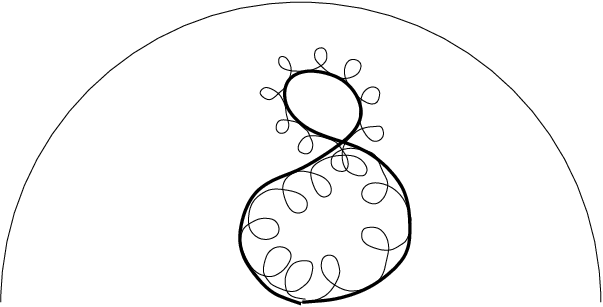
We now present a more rigorous version of this argument. Let ${\cal C}_{0}$ be the circle with diameter $e_{1}e_{3}$, parametrized by $\nu_{1}\in{\cal L}_{I}$,

$$\nu_{1}(t)=\left(\frac{1+\cos(2\pi t)}{2},\frac{\sqrt{2}}{2}\sin(2\pi t),\frac{1-\cos(2\pi t)}{2}\right).$$

For positive $n$, let $\nu_{n}(t)=\nu_{1}(nt)$ so that $\nu_{1}\in{\cal L}_{-1,c}$ and, for $n>1$, $\nu_{n}\in{\cal L}_{(-1)^{n}}$.

For $\gamma_{1}\in{\cal I}_{\sigma_{1}}$, $\gamma_{2}\in{\cal I}_{\sigma_{2}}$, $\sigma_{i}\in\{+1,-1\}$, let $\gamma_{1}\ast\gamma_{2}\in{\cal I}_{\sigma_{1}\sigma_{2}}$ be defined by

$$(\gamma_{1}\ast\gamma_{2})(t)=\begin{cases}\gamma_{1}(2t),&0\leq t\leq 1/2,\\ \gamma_{2}(2t-1),&1/2\leq t\leq 1.\end{cases}$$

Notice that if $\gamma_{1},\gamma_{2}\in{\cal L}_{I}$ then $\gamma_{1}\ast\gamma_{2}\in{\cal L}_{I}$. For $f:K\to{\cal I}_{I}$, let $\nu_{n}\ast f:K\to{\cal I}_{I}$ be defined by $(\nu_{n}\ast f)(p)=\nu_{n}\ast(f(p))$. The observation in Figure 4 can be translated as the following lemma, whose straightforward proof will be omitted.

We now need a construction corresponding to adding loops along the curve, as in Figure 5. For $\gamma\in{\cal I}_{\pm}$ and $n>0$, define $(F_{n}(\gamma))(t)={\mathfrak{F}}_{\gamma}(t)\nu_{n}(t)$.

For $\gamma=f(k)$, write

$$\tilde{\gamma}(t)=(F_{2n}\gamma)(t)={\mathfrak{F}}_{\gamma}(t)\nu_{2n}(t)={\mathfrak{F}}_{\gamma}(t)\nu_{1}(2nt)$$

so that

	$\displaystyle\tilde{\gamma}^{\prime}(t)$	$\displaystyle={\mathfrak{F}}_{\gamma}^{\prime}(t)\nu_{1}(2nt)+2n{\mathfrak{F}}_{\gamma}(t)\nu_{1}^{\prime}(2nt)$
	$\displaystyle\tilde{\gamma}^{\prime\prime}(t)$	$\displaystyle={\mathfrak{F}}_{\gamma}^{\prime\prime}(t)\nu_{1}(2nt)+4n{\mathfrak{F}}_{\gamma}^{\prime}(t)\nu_{1}^{\prime}(2nt)+4n^{2}{\mathfrak{F}}_{\gamma}(t)\nu_{1}^{\prime\prime}(2nt)$

and therefore, after a few manipulations,

$$\left|\frac{\tilde{\gamma}^{\prime}(t)}{2n}-{\mathfrak{F}}_{\gamma}(t)\nu_{1}^{\prime}(2nt)\right|<\epsilon,\quad\left|\frac{\tilde{\gamma}^{\prime\prime}(t)}{4n^{2}}-{\mathfrak{F}}_{\gamma}(t)\nu_{1}^{\prime\prime}(2nt)\right|<\epsilon$$

or, equivalently,

$$\left|\frac{({\mathfrak{F}}_{\gamma}(t))^{-1}\tilde{\gamma}^{\prime}(t)}{2n}-\nu_{1}^{\prime}(2nt)\right|<\epsilon,\quad\left|\frac{({\mathfrak{F}}_{\gamma}(t))^{-1}\tilde{\gamma}^{\prime\prime}(t)}{4n^{2}}-\nu_{1}^{\prime\prime}(2nt)\right|<\epsilon.$$

It follows that

$$\det\left(\nu_{\theta}(2nt),\frac{({\mathfrak{F}}_{\gamma}(t))^{-1}\tilde{\gamma}^{\prime}(t)}{2n},\frac{({\mathfrak{F}}_{\gamma}(t))^{-1}\tilde{\gamma}^{\prime\prime}(t)}{4n^{2}}\right)>0$$

and therefore that $\det(\tilde{\gamma}(t),\tilde{\gamma}^{\prime}(t),\tilde{\gamma}^{\prime\prime}(t))>0$, which is what we needed.     $\blacksquare$

Theorem 1 now follows directly from the next lemma.

This completes the proof of Theorem 1. For later use, we want a geometric understanding of what this tells us about $H^{2}({\cal L}_{\pm 1})$.

Recall that $H_{2}({\cal I}_{\pm 1};{\mathbb{Z}})=\pi_{2}({\cal I}_{\pm 1})=\pi_{2}(\Omega{\mathbb{S}}^{3})={\mathbb{Z}}$. Since an element of $\Omega{\mathbb{S}}^{3}$ is a function from ${\mathbb{S}}^{1}$ to ${\mathbb{S}}^{3}$, a map $\alpha:{\mathbb{S}}^{2}\to\Omega{\mathbb{S}}^{3}$ can be reinterpreted as a map $\hat{\alpha}:{\mathbb{S}}^{2}\times{\mathbb{S}}^{1}\to{\mathbb{S}}^{3}$. The identification between $\pi_{2}(\Omega{\mathbb{S}}^{3})$ and ${\mathbb{Z}}$ takes such a map $\alpha$ to the degree of $\hat{\alpha}$.

Similarly, let $M$ be a closed oriented surface and consider a map $\beta:M\to{\cal I}_{+1}$. Let $\hat{\beta}:M\times{\mathbb{S}}^{1}\to{\mathbb{S}}^{3}$ be defined by $\hat{\beta}(p,t)=\tilde{\mathfrak{F}}_{\beta(p)}(t)$. Define ${\mathbf{x}}:H_{2}({\cal I}_{+1};{\mathbb{Z}})\to{\mathbb{Z}}$ by ${\mathbf{x}}(\beta)=\deg(\hat{\beta})$: the map ${\mathbf{x}}$ provides the identification $H_{2}({\cal I}_{+1};{\mathbb{Z}})={\mathbb{Z}}$ and is a generator of $H^{2}({\cal I}_{+1};{\mathbb{Z}})$. A similar construction defines ${\mathbf{x}}\in H^{2}({\cal I}_{-1};{\mathbb{Z}})$. The inclusion ${\cal L}_{\pm 1}\subset{\cal I}_{\pm 1}$ defines ${\mathbf{x}}\in H^{2}({\cal L}_{\pm 1};{\mathbb{Z}})$.

As we shall see later, a function $f:K\to{\cal L}_{I}\subset{\cal I}_{I}$ may be homotopic to a constant in ${\cal I}_{I}$ but not in ${\cal L}_{I}$. The following proposition shows that this changes if we add loops.

On the other hand, as we observed in Figure 3, one loop can be converted to three loops. The interval $[0,1/2]$ counts as a loop in $\nu_{1}\ast f$ and therefore $\nu_{1}\ast f$ is homotopic in ${\cal L}_{I}$ to $\nu_{3}\ast f$. More generally, $\nu_{n}\ast f$ is homotopic to $\nu_{n+2}\ast f$, completing the proof.     $\blacksquare$

Recall that a curve $\gamma\in{\cal L}_{(-1)^{(k+1)}}$ is a flower of $2k+1$ petals if there exist $0=t_{0}<t_{1}<t_{2}<\cdots<t_{2k}<t_{2k+1}=1$ and $0=\theta_{0}<\theta_{1}<\theta_{2}<\cdots<\theta_{2k}<\theta_{2k+1}=\theta_{M}$ such that:

1. 1.

   $\gamma(t_{1})=\gamma(t_{2})=\cdots=\gamma(t_{2k})=e_{1}$;

2. 2.

   the only self-intersections of the curve $\gamma$ are of the form $\gamma(t_{i})=\gamma(t_{j})$;

3. 3.

   the argument of $(x_{i,2},x_{i,3})$ is $\theta_{i}$, where $(0,x_{i,2},x_{i,3})=(-1)^{i}\gamma^{\prime}(t_{i})$.

For $i=0,\ldots,2k$, it follows from Section 2 that the restrictions $\gamma|_{[t_{i},t_{i+1}]}$ (the petals) are convex curves. Let ${\cal F}_{2k}\subset{\cal L}_{(-1)^{(k+1)}}$ be the set of flowers with $2k+1$ petals.

Near a flower $\gamma_{0}$, curves $\gamma$ will intersect the large circle through $e_{1}$ and $e_{2}$ transversally (see Figure 6). Let $\eta_{0}(t)=\langle\gamma(t),e_{3}\rangle$: we have $2k$ solutions $\hat{t}_{i}\approx t_{i}$ to $\eta_{0}(\hat{t})=0$ (where $\gamma_{0}(t_{i})=e_{1}$). Define

$$\psi_{2k}(\gamma)=\left(\langle\gamma(\hat{t}_{1}),e_{2}\rangle,\langle\gamma(\hat{t}_{2}),e_{2}\rangle,\ldots,\langle\gamma(\hat{t}_{2k}),e_{2}\rangle\right).$$

Clearly, $\psi_{2k}(\gamma)=0$ if and only if $\gamma$ is a flower. The regularity of the value $0$ follows from the fact that the curves are transversal to the horizontal plane at $\hat{t}_{i}$, completing the proof.     $\blacksquare$

The sets ${\cal F}_{2k}$ are contractible: this follows from the fact that the space of possible petals (convex curves) is contractible ([15]) for every choice of $t_{1},\ldots,t_{2k}$ and $\theta_{1},\ldots,\theta_{2k}$. We shall not use this fact in this paper; it will be proved in [10].

Counting intersections with ${\cal F}_{2k}$ defines an element ${\mathbf{f}}_{2k}$ in $H^{2k}({\cal L}_{(-1)^{(k+1)}};{\mathbb{Z}})$. Since the sets ${\cal F}_{2k}$ are disjoint and the normal bundle is trivial we have ${\mathbf{f}}_{2k}{\mathbf{f}}_{2k^{\prime}}=0$ both for $k\neq k^{\prime}$ and $k=k^{\prime}$. Also, the degree of $\hat{\beta}:M\times{\mathbb{S}}^{1}\to{\mathbb{S}}^{3}$ (as in the definition of ${\mathbf{x}}$) can be computed at an element $z\in{\mathbb{S}}^{3}$ with

$$\Pi(z)=\begin{pmatrix}-1&0&0\\ 0&1&0\\ 0&0&-1\end{pmatrix};$$

since no flower ever passes through the point $-e_{1}$, we have ${\mathbf{x}}{\mathbf{f}}_{2k}=0$. We still have to prove that ${\mathbf{f}}_{2k}\neq 0$.

It is probably good to begin by recalling Little’s proof that $\nu_{2}$ (a circle drawn twice) and $\nu_{4}$ (a circle drawn four times) are in the same connected component of ${\cal L}_{I}$. Figure 7 below illustrates this. Initially perturb your curve in order to have three self-intersection points forming approximately an equilateral triangle. Pull out the “petals” to obtain a flower with three petals, as in the third figure. Pull the petals even further so that you have a curvilinear triangle with loops at the three vertices. The passage from the fourth to the fifth figure is the only one where it is important to recall that we are in a sphere, not in the plane: one way to think of this is that the triangle became large and the bulk of the sphere passed through the triangle. Now it is merely a matter of bringing the three loops together and making the curve round again.

In the construction of this path there was one important arbitrary choice: the position of the base point, or, equivalently, the orientation of the triangle. From either point of view, the construction can be turned producing a continuous family indexed by ${\mathbb{S}}^{1}$ of such paths. Since the endpoints of all paths coincide, this is equivalent to constructing a map ${\mathbf{g}}_{+,2}:{\mathbb{S}}^{2}\to{\cal L}_{+1}$, with the two poles taken to $\nu_{2}$ and $\nu_{4}$, meridians (from one pole to the other) corresponding to paths like the one in Figure 7 and parallel circles being taken to paths obtained by rotating the curve an in Figure 8.

The whole construction is illustrated in Figure 9. The leftmost and rightmost columns are adjacent, the north pole $\nu_{4}$ is at the top and the south pole $\nu_{2}$ is at the bottom (as in most world maps). In the transition between the first and second rows most of the curve passed around the back of the sphere.

As an alternative to this figure, we provide a formula for ${\mathbf{g}}_{+,2}$. Let $\alpha:[0,1]\times[0,1]\to SO(3)$ be defined by

$$\alpha(s,t)=\begin{pmatrix}\sin\pi s\cos 2\pi t&-\sin 2\pi t&-\cos\pi s\cos 2\pi t\\ \sin\pi s\sin 2\pi t&\cos 2\pi t&-\cos\pi s\sin 2\pi t\\ \cos\pi s&0&\sin\pi s\end{pmatrix}$$

and define

$$\gamma_{s}(t)=\frac{\sqrt{2}}{2}\;\alpha(s,t)\begin{pmatrix}1\\ \cos 6\pi t\\ \sin 6\pi t\end{pmatrix}.$$

The curve $\gamma_{0}$ is a circle drawn $4$ times and the curve $\gamma_{1}$ is a circle drawn $2$ times. A tedious but straightforward computation verifies that the curves $\gamma_{s}$ are closed and locally convex and therefore belong to ${\cal L}_{per}$.

Let $\Gamma(s,t)={\mathfrak{F}}_{\gamma_{s}}(t)$: it easy to verify that

$$\Gamma(s,t+(1/3))=\begin{pmatrix}-1/2&-\sqrt{3}/2&0\\ \sqrt{3}/2&-1/2&0\\ 0&0&1\end{pmatrix}\Gamma(s,t)$$

for all $s$ and $t$. Finally, let ${\mathbf{g}}_{+,2}:[0,1]\times[0,1]\to{\cal L}_{+1}$ be defined by

$${\mathbf{g}}_{+,2}(s_{1},s_{2})(t)=(\Gamma(s_{2},s_{1}/3))^{-1}\Gamma(s_{2},t+(s_{1}/3))e_{1}.$$

If $s_{2}=0$ or $1$, the value of $s_{1}$ is irrelevant for the value of ${\mathbf{g}}_{+,2}$. Also, ${\mathbf{g}}_{+,2}(0,s_{2})={\mathbf{g}}_{+,2}(1,s_{2})$ for all $s_{2}$. Performing these identifications, the domain of ${\mathbf{g}}_{+,2}$ becomes the sphere ${\mathbb{S}}^{2}$, as required.

It follows easily either from Figure 9 or from the formulas that ${\mathbf{x}}({\mathbf{g}}_{+,2})=1$, i.e., that the degree of $\hat{\mathbf{g}}_{+,2}:{\mathbb{S}}^{2}\times{\mathbb{S}}^{1}\to{\mathbb{S}}^{3}$, $\hat{\mathbf{g}}_{+,2}(p,t)=\tilde{\mathfrak{F}}_{{\mathbf{g}}_{+,2}(p)}(t)$, equals $1$. This can be seen, for instance, by computing preimages of some $z\in{\mathbb{S}}^{3}$. Thus, ${\mathbf{g}}_{+,2}$ is a generator of $\pi_{2}({\cal I}_{+1})$.

It is again clear from Figure 9 that ${\mathbf{g}}_{+,2}$ intersects ${\cal F}_{2}$ precisely once (the flower is in the third row, first column), and the intersection is transversal, and therefore $|{\mathbf{f}}_{2}({\mathbf{g}}_{+,2})|=1$. We were not too careful about the orientation of ${\mathbf{f}}_{2}$ in Section 4 so we decree now that ${\mathbf{f}}_{2}({\mathbf{g}}_{+,2})=1$. This can likewise be checked for the formula by a long and tedious computation which we skip. Either way, ${\mathbf{f}}_{2}\neq 0$.

Consider the function $\nu_{2}\ast{\mathbf{g}}_{+,2}$. We have ${\mathbf{x}}(\nu_{2}\ast{\mathbf{g}}_{+,2})=1$ (adding these loops does not change the degree) and ${\mathbf{f}}_{2}(\nu_{2}\ast{\mathbf{g}}_{+,2})=0$ (there are no flowers in the image of $\nu_{2}\ast{\mathbf{g}}_{+,2}$ since no flower starts with two loops). In particular, the maps ${\mathbf{g}}_{+,2}$ and $\nu_{2}\ast{\mathbf{g}}_{+,2}$ are not homotopic in ${\cal L}_{+1}$. On the other hand, from Lemma 3.1, the maps ${\mathbf{g}}_{+,2}$ and $\nu_{2}\ast{\mathbf{g}}_{+,2}$ are homotopic in ${\cal I}_{+1}$.

We will now consider the group $\pi_{2}({\cal L}_{+1})$ but before we do so we must say a few words about base points. Recall that given two base points $p_{1}$ and $p_{2}$, the two homotopy groups $\pi_{2}({\cal L}_{+1};p_{1})$ and $\pi_{2}({\cal L}_{+1};p_{2})$ are identified via a homotopy class of paths from $p_{1}$ to $p_{2}$. We prove in [10] that ${\cal L}_{+1}$ and ${\cal L}_{-1,n}$ are simply connected and therefore the identification is natural; the idea here is not, however, to use these results. We shall therefore select $\nu_{2}$ as a base point for ${\cal L}_{+1}$ and $\nu_{3}$ as a base point for ${\cal L}_{-1}$.

References

- [1] Bott, R. and Tu, L., Differential forms in algebraic topology, Spinger-Verlag, GTM 82, New York, 1982.
- [2] Burghelea, D., Saldanha, N. and Tomei, C., The topology of the monodromy map of a second order ODE, J. Differential Equations 227, 581-597 (2006).
- [3] Burghelea, D., Saldanha, N. and Tomei, C., The geometry of the critical set of nonlinear periodic Sturm-Liouville operators, J. Differential Equations 246, 3380-3397 (2009).
- [4] Eliashberg, Ya., Mishachev, N., Introduction to the h-principle, Graduate Studies in Mathematics, 48. American Mathematical Society, Providence, RI, 2002. xviii+206 pp.
- [5] Gromov, M., Partial Differential Relations, Springer-Verlag, 1986.
- [6] Hirsch, M., Immersions of manifolds, Trans. Am. Math. Soc. 93, 242-276, 1959.
- [7] Little, J. A., Nondegenerate homotopies of curves on the unit 2-sphere, J. Differential Geometry, 4, 339-348, 1970.
- [8] Morse, M., The calculus of variations in the large. Reprint of the 1932 original. American Mathematical Society Colloquium Publications, 18. American Mathematical Society, Providence, RI, 1996. xii+368 pp.
- [9] Saldanha, N., The homotopy type of spaces of locally convex curves in the sphere, in preparation.
- [10] Saldanha, N., The cohomology of spaces of locally convex curves in the sphere — II, preprint, arXiv:0905.2116v1.
- [11] Saldanha, N. and Shapiro, B., Spaces of locally convex curves in and combinatorics of the group , Journal of Singularities, 4, 1-22, 2012.
- [12] Saldanha, N. and Tomei, C., The topology of critical sets of some ordinary differential operators, Progress in Nonlinear Differential Equations and Their Applications, 66, 491-504 (2005).
- [13] Shapiro, B. and Khesin, B., Homotopy classification of nondegenerate quasiperiodic curves on the -sphere, Publ. Inst. Math. (Beograd) 66(80), 127-156, 1999.
- [14] Shapiro, B. and Shapiro, M., On the number of connected components of nondegenerate curves on , Bull. of the AMS, 25, 75-79, 1991.
- [15] Shapiro, M., Topology of the space of nondegenerate curves, Math. USSR, 57, 106-126, 1993.
- [16] Smale, S., The classification of immersions of spheres in euclidean spaces, Ann. of Math. 69, 327-344, 1959.
Nicolau C. Saldanha, PUC-Rio
saldanha@puc-rio.br; http://www.mat.puc-rio.br/nicolau/
Departamento de Matemática, PUC-Rio
R. Marquês de S. Vicente 225, Rio de Janeiro, RJ 22453-900, Brazil