Spectral methods for volatility derivativesThanks: The authors would like to thank all three referees for lucid and constructive comments. AM would also like thank Jim Gatheral for useful conversations.

Claudio Albanese Address: Independent consultant Email address: claudio_albanese@hotmail.co.uk , Harry Lo Address: Imperial College London and Swiss Re Email address: lo.harry@gmail.com and Aleksandar Mijatović Address: Department of Mathematics, Imperial College London Email address: a.mijatovic@imperial.ac.uk

Abstract.

In the first quarter of 2006 Chicago Board Options Exchange (CBOE) introduced, as one of the listed products, options on its implied volatility index (VIX). This created the challenge of developing a pricing framework that can simultaneously handle European options, forward-starts, options on the realized variance and options on the VIX. In this paper we propose a new approach to this problem using spectral methods. We use a regime switching model with jumps and local volatility defined in [1] and calibrate it to the European options on the S&P 500 for a broad range of strikes and maturities. The main idea of this paper is to “lift” (i.e. extend) the generator of the underlying process to keep track of the relevant path information, namely the realized variance. The lifted generator is too large a matrix to be diagonalized numerically. We overcome this difficulty by applying a new semi-analytic algorithm for block-diagonalization. This method enables us to evaluate numerically the joint distribution between the underlying stock price and the realized variance, which in turn gives us a way of pricing consistently European options, general accrued variance payoffs and forward-starting and VIX options.

1. Introduction

In recent years there has been much interest in trading derivative products whose underlying is a realized variance of some liquid financial instrument (e.g. S&P 500) over the life of the contract. The most popular payoff functions¹¹ 1 For the precise definition of these products see Appendices B.1 and B.2. are linear, leading to variance swaps, square root, yielding volatility swaps, and the usual put and call payoffs defining variance swaptions.

It is clear that the plethora of possible derivatives on the realized variance is closely related to the standard volatility-sensitive instruments like vanilla options, which are also exposed to other market risks, and the forward-starting options which are almost pure vega bets and are mainly exposed to the movements of the forward smile. Recently Chicago Board Options Exchange (CBOE) introduced options on the volatility index²² 2 For a brief description of the these securities see Appendix B.3. For the definition of VIX see [12]. (VIX) which are also important predictors for the future behaviour of implied volatility. The main purpose of this paper is to introduce a framework in which all of the above financial instruments (i.e. the derivatives on the realized variance as well as the instruments depending on the implied volatility) can be priced and hedged consistently and efficiently.

Our central idea is very simple and can be described as follows. We use a model for the underlying that includes local volatility, stochastic volatility (i.e. regime switching) and jumps and can be calibrated to the implied volatility surface for a wide variety of strikes and maturities (for the case of European options on the S&P 500 see Figure 1). The stochastic process for the underlying is a continuous-time Markov chain, as defined in [1], where it was used for modelling the foreign exchange rates. The underlying process is stationary as can be inferred from the fact that the implied forward volatility smile behaves in a consistent way (see Figures 7, 8, 9 and 10).

There are two features of this model that make it possible to obtain the distributions of the future behaviour of the implied volatility and the realized variance of the underlying. The first feature is the complete numerical solubility of the model. In other words spectral theory provides a simple and efficient algorithm (see [1], Section 3) for obtaining a conditional probability distribution function for the underlying between any given pair of times in the future. This property is sufficient to determine completely the forward volatility smile and the distribution of VIX for any maturity. The second feature of the framework is that it allows us to describe the realized variance of the underlying risky security as a continuous-time Markov chain. This makes it possible to deal with the realized variance by extending the generator of the original process and thus obtaining a new continuous-time Markov chain which keeps track simultaneously of the realized variance and the underlying forward rate.

The key idea of the paper is to assume that the state-space of the realized variance process lies on a circle. This allows us to apply a block-diagonalization algorithm (described in detail in Appendix A) and the standard methods from spectral theory to obtain a joint probability distribution function for the underlying process and its realized variance or volatility at any time in the future (e.g. for time horizons of 6 months and 1 year see Figure 15). This joint pdf is precisely what is needed to price a completely general payoff that depends on the realized variance and on the underlying.

There are two natural and useful consequences of this approach. One is that we do not need to specify exogenously the process for the variance and then try to find an arbitrage-free dynamics for the underlying, but instead imply such a process from the observed vanilla market via the model for the underlying (a term-structure of the fair values of variance swaps as implied by the vanilla market data and our model is shown in Figure 18). The second consequence is that this approach bypasses the use of Monte Carlo techniques and therefore yields sharp and easily computable sensitivities of the volatility derivatives to the market parameters. This is because the pricing algorithm yields, as a by-product, all the necessary information for finding the required hedge ratios.

There is a rapidly growing interest in trading volatility derivatives in financial markets, mainly a consequence of the following two factors. On the one hand, pure volatility instruments are used to hedge the implicit vega exposure of the portfolios of market participants, thus eliminating the need to trade frequently in the vanilla options market. This in itself is advantageous because of the relatively large bid-offer spreads prevailing in that market. On the other hand, volatility derivatives are a useful tool for speculating on future volatility levels and for trading the difference between realized and implied volatility.

This interest is reflected in the vast amount of literature devoted to volatility products. The analysis of the realized variance is intrinsically easier than that of realized volatility because of the additivity of the former. Under the hypothesis that the underlying price process is continuous the realized variance can be hedged perfectly by a European contract with the logarithmic payoff first studied in [26] and a dynamic trading strategy in the underlying. This approach does not require an explicit specification for the instantaneous volatility process of the underlying and can therefore be used within any stochastic volatility framework. This idea has been developed in [11] and [14], where the static replication strategy for the log contract, using calls and puts, is described. Types of mark-to-market risk faced by a holder of a variance swap are studied and classified in [13]. A direct delta-hedging approach for the realized variance is given in [22]. A shortcoming of pricing variance swaps without specifying a volatility model (as described in [11] and [15]) is that this methodology does not yield a natural method for the computation of the sensitivities to market parameters (i.e. the Greeks). In [23] a diffusion model for the volatility process is specified that allowed the authors to use PDE technology to price and hedge variance and volatility swaps, as well as more general payoffs. Derivatives on the realized volatility can be considered naturally as derivatives on the square root of the realized variance. In [6] the authors provide a volatility convexity correction which relates the two families of derivatives. Another approach, pioneered in [9], develops a robust hedging strategy for volatility derivatives which is analogous to the one for variance swaps. This method works for continuous processes only and is based on the observation that, under the continuity hypothesis, there is a simple algebraic relationship between the Laplace transform of the process and the Laplace transform of its quadratic variation. There are some technical difficulties in computing the relevant integrals, which have been dealt with in [18]. In [31] the authors investigate hedging techniques for discretely monitored volatility contracts that are independent of the instantaneous volatility dynamics. Another model-independent hedging approach in an environment with jumps for variance swaps is presented in [29]. A modelling framework, analogous to the HJM, for the term-structure of variance swaps has been proposed in [7]. The starting point is the specification of the function-valued process for the forward instantaneous variance, which yields an arbitrage-free dynamics for the underlying. In order to be calibrated, this model requires at time zero the entire variance swap curve.

The paper is organized as follows. The key idea that allows us to price general derivatives on the realized variance is introduced in Section 2. Section 3 explains the pricing algorithm, based on Theorem 3.1, for derivatives on the realized variance. In Section 4 we discuss the calibration of the model to a wide range of strikes and maturities for options written on the S&P 500. In Section 5 we carry out numerical experiments and consistency tests on the calibrated model, including a comparison with a Monte Carlo method (see Subsection 5.6). Concluding remarks are contained in Section 6. The numerical algorithm required to make this idea applicable is described in Appendix A, which also contains the proof of Theorem 3.1. Appendix B describes some of the volatility contracts that can be priced within our framework and are referred to throughout the paper.

2. The variance process for continuous-time Markov chains

As mentioned in the introduction the main idea of this paper is to describe the realized variance of the underlying risky security as a continuous-time Markov chain on a state-space which lies on a circle. The model for the underlying $F_{t}$ will be given in the forward measure as a mixture of local and stochastic volatility coupled with an infinite activity jump process. It will be defined on a continuous-time lattice in a largely non-parametric fashion, as described in [1], where it was used for modelling the foreign exchange rate. We will briefly recall the definition of the model in Section 3 and describe its calibration to the vanilla surface on the S&P 500 in Section 4.

In the current section and the one that follows our task is to build a mechanism that will make it possible to identify the random behaviour of the realized variance of the process $F_{t}$ . The approach we take will only use the fact that the process $F_{t}$ is a continuous-time Markov chain and will not depend on any other properties of the process. In order to do this we must return briefly to the fundamental theory (see [27], Chapters 2 and 3, for background on continuous-time Markov chains).

Let $\mathcal{L}$ be a generator for a continuous-time Markov chain $F_{t}$ defined on a finite state space $\Omega$ . In other words the operator $\mathcal{L}$ is given by a square matrix $(\mathcal{L}(x,y))_{x,y\in\Omega}$ which satisfies probability conservation and has non-negative elements off the diagonal. Each element $\mathcal{L}(x,y)$ describes the first order change of the probability that the chain $F_{t}$ jumps from level $F(x)$ to the level $F(y)$ in the time interval $[t,t+dt]$ , where the deterministic function $F:\Omega\rightarrow(0,\infty)$ is an injection which defines the image of the process $F_{t}$ .

Our aim in this section is to extend (i.e. lift) the generator $\mathcal{L}$ to the generator $\widetilde{\mathcal{L}}$ , which will describe the dynamics of the lifting $(F_{t},I_{t})$ of our original process $F_{t}$ . The component $I_{t}$ will be a finite-state continuous-time Markov chain, which will be described shortly, that approximates the realized variance, up to time $t$ , of the underlying process $F_{t}$ . The generator of the chain $(F_{t},I_{t})$ will give us the probability kernel for the process $I_{t}$ , which is what we are ultimately interested in as it contains the probability distribution of the relevant path information.

We will start by describing a continuous process $\Sigma_{t}$ which will contain the relevant path-information of the underlying Markov chain $F_{t}$ and then define a finite-state stochastic process $I_{t}$ that will be used to approximate $\Sigma_{t}$ . The key feature of the state-space of the process $I_{t}$ , which allows numerical tractability of our approach, is that it is contained on a circle in the complex plane (see Section 3).

The procedure we are about to describe works for a specific type of path-dependence only. Assume that if at time $t$ the underlying process $F_{t}$ is at a state $F(x)$ for some $x\in\Omega$ , then the change of the value $\Sigma_{t}$ , in the infinitesimal time interval $dt$ is of the form

d\Sigma_{t}=Q(x)dt,

where the function $Q:\Omega\rightarrow\mathbb{R}$ , defined in terms of the underlying stochastic process, has two key properties:

•

the mapping $Q$ is independent of the path the underlying process follows on the interval $[0,t)$ and
•

the value $Q(x)$ depends on the level $x$ at time $t$ and on the distribution of the underlying process in the infinitesimal future time interval $dt$ as given by the Markov generator $\mathcal{L}$ .

The first property states that the change in the path-information $\Sigma_{t}$ , over a short time period $[t,t+dt]$ , does not depend on the path taken by the underlying process up to time $t$ . The second property tells us that the evolution of the path information over the interval $[t,t+dt]$ , conditional on the current level of the process $F_{t}$ , is determined by the future distribution of $F_{t}$ over the infinitesimal time interval.

It is clear that the realized variance of the process $F_{t}$ up to time $t$ , can be captured by a random process $\Sigma_{t}$ . Indeed, if we define the function $Q$ in the following way

(1)

\displaystyle Q(x):=\sum_{y\in\Omega}\left(\frac{F(y)-F(x)}{F(x)}\right)^{2}\mathcal{L}(x,y)

it follows immediately that the above conditions are satisfied. This is because the realized variance of $F_{t}$ is simply an integral over time of the instantaneous variance of $F_{t}$ which is given by (1).

The last observation is crucial for all that follows, because it implies that the process $\Sigma_{t}$ is uniquely determined by its state-dependent instantaneous drift. In particular we see that the process $\Sigma_{t}$ has no volatility term and that it has continuous sample paths since it allows a representation as an integral over time.

The fundamental consequence of these facts is the following: a finite-state Markov chain $I_{t}$ can be used as a model for the process $\Sigma_{t}$ if and only if the instantaneous drift of the chain is equal to $Q(x)$ , whenever the underlying process $F_{t}$ is in state $F(x)$ , and the instantaneous variance of $I_{t}$ is equal to zero up to first order. The first requirement clearly follows from the discussion above. The second condition is there to reflect the fact that the process $\Sigma_{t}$ is a continuous Itô process which has no volatility term. A non-constant random process on a lattice will always have a non-zero instantaneous variance, but the second condition ensures that this instantaneous variance goes to zero as quickly as the lattice spacing itself. In other words the Markov chain approximation $I_{t}$ for the process $\Sigma_{t}$ must exhibit neither diffusion nor jump behaviour. Therefore, as we shall see in the next subsection, $I_{t}$ must be a Poisson process with state-dependent intensity.

2.1. Lifting of the generator for the underlying process

Let $I_{t}$ as above denote the Markov chain whose value approximates the realized variance $\Sigma_{t}$ of the forward price $F_{t}$ from time $0$ to time $t$ . We shall express $I_{t}$ as $\alpha m_{t}$ where $m_{t}$ is a Poisson process (with non-constant intensity) starting at $0$ and gradually jumping up along the grid given by $\Psi=\{0,\ldots,2C\}$ , where $C$ is an element in $\mathbb{N}$ . The constant $\alpha$ controls the spacing of the grid for the realized variance $I_{t}$ .

We are now going to specify precisely the dynamics of the process $m_{t}$ which is a fundamental ingredient of our model. As mentioned before, the process $m_{t}$ will behave as a Poisson process whose intensity is determined by the level of the underlying. In other words the Markov generator, conditional on the underlying process being at the level $F(x)$ , is of the form

\displaystyle\mathcal{L}^{m}(x:c,d):=\left\{\begin{array}[]{ll}\frac{1}{\alpha}Q(x)&\mathrm{if}\>\>d=(c+1)\!\!\!\mod(2C+1);\\ &\\ -\frac{1}{\alpha}Q(x)&\mathrm{if}\>\>d=c.\end{array}\right.

The variables $c$ and $d$ are elements of the discrete set $\Psi=\{0,\ldots,2C\}$ and the function $Q$ is the instantaneous variance of the underlying process as defined in (1). This family of generators specifies the dynamics of the process $I_{t}$ with the following instantaneous drift

(6)		$\displaystyle\lim_{\Delta t\rightarrow 0}\mathbb{E}\left[\frac{I_{t+\Delta t}-I_{t}}{\Delta t}\Bigl\lvert F_{t}=F(x),I_{t}=I(c)\right]$	$\displaystyle=$	$\displaystyle\sum_{d=0}^{2C}(I(d)-I(c))\mathcal{L}^{m}(x:c,d)$
(6)			$\displaystyle=$	$\displaystyle\alpha(c+1-c)\frac{1}{\alpha}Q(x)=Q(x),$

for all values $F(x)$ of the underlying process $F_{t}$ and all integers $c$ which are strictly smaller than $2C$ . This implies that the Markov chain $I_{t}$ has the same instantaneous drift as the actual realized variance. A similar calculation tells us that the instantaneous variance of $I_{t}$ equals $\alpha Q(x)$ . Since $\alpha$ is the spacing of the lattice for the chain $I_{t}$ , we have just shown that the first two instantaneous moments of $I_{t}$ match the first two moments of the realized variance $\Sigma_{t}$ for all points on the lattice $\{0,\ldots,2C\}$ except the last one.

Notice however that the equality (6) breaks down if $c$ equals $2C$ , because we have imposed periodic boundary condition for the process $I_{t}$ . Put differently this means that $I_{t}$ is in fact a process on a circle rather than on an interval. The latter would be achieved if we had imposed absorbing boundary conditions at $2C$ . That would perhaps be a more natural thing to do since the process $\Sigma_{t}$ is certainly not periodic. But an absorbing boundary condition would destroy the delicate structure of the spectrum of the lifted generator $\widetilde{\mathcal{L}}$ which is preserved by the periodic boundary condition. It is precisely this structure that makes the periodic nature of $I_{t}$ a key ingredient of our model, because it allows us to linearize the complexity of the pricing algorithm (see appendix A). It should be noted that the general philosophy behind either choice of the boundary condition would be the same: the lattice in the calibrated model should be set up in such a way that the process never reaches the boundary value $2C$ , because if it does an inevitable loss of information will ensue regardless of the boundary conditions we choose.

We are now finally in a position to define the lifted Markov generator of the process $(F_{t},I_{t})$ as

(7)

\displaystyle\widetilde{\mathcal{L}}(x,c;y,d):=\mathcal{L}(x,y)\delta_{c,d}+\mathcal{L}^{m}(x:c,d)\delta_{x,y},

where $x,y$ are in the state-space of the chain $F_{t}$ and $c,d$ are elements in $\Psi$ . The structure of the spectrum of the operator $\widetilde{\mathcal{L}}$ will be exploited in Section 3 to obtain a pricing algorithm for payoffs which are general functions of the realized variance (see Theorem 3.1). The reason for specifying the generator $\mathcal{L}^{m}(x:c,d)$ by (2.1) (i.e. insisting on the periodic boundary condition for the process $I_{t}$ ) will become clear in the proof of Theorem 3.1, which exploits the spectral properties of the lifted generator $\widetilde{\mathcal{L}}$ (see appendix A for the precise description of the spectrum of $\widetilde{\mathcal{L}}$ ).

3. Pricing of derivatives on realized variance

Recall that the generator $\mathcal{L}$ for the underlying continuous-time Markov chain $F_{t}$ in the forward measure, described in [1], is defined on the state-space $\Omega\times V$ via an injective function $F:\Omega\times V\rightarrow(0,\infty)$ . The set $\Omega$ with $N$ elements is the state-space of the various jump-diffusions and the set $V$ with $M$ elements is the state-space for the random switching between regimes (see the formulae on page 7 in [1] for the precise definition of the generator matrix $(\mathcal{L}(x,\beta;y,\gamma))_{(x,\beta),(y,\gamma)\in\Omega\times V}$ ). In Section 4 we shall see that for the options data on the S&P 500 used in this paper, it suffices to take $N=76$ with only two regimes ( $M=2$ ).

Let $\Sigma_{T}$ be the realized variance over the time interval $[0,T]$ , expressed in annual terms, as defined in (19). In this section we are going to find pricing formulae for general payoffs that depend on the annualized realized variance $\Sigma_{T}$ .

Our first task is to find the probability kernel of the lifted process $(F_{t},I_{t})$ which was defined in Section 2. Recall that the Markov chain $I_{t}=\alpha m_{t}$ , which is used to model the realized variance, is specified in terms of a translation invariant process $m_{t}$ , whose domain is $\Psi=\{0,\ldots,2C\}$ , and some positive constant $\alpha$ which determines the lattice spacing for the domain of $I_{t}$ . The value $C\in\mathbb{N}$ specifies the size of the lattice for the realized variance and has to be large enough so that the process $I_{t}$ , starting from zero, does not transverse the entire lattice. This is a very important technical requirement as it ensures that there is no probability leakage in the model (which is theoretically possible since we are using periodic boundary conditions for the process $I_{t}$ ). The dynamics of the chain $m_{t}$ are given by the Markov generator in (2.1).

Recall also that the process $I_{t}$ records the total realized variance up to time $t$ , which implies that the annualized realized variance $\Sigma_{T}$ that interests us, will be described by $\frac{1}{T}I_{T}$ where the time horizon $T$ is expressed in years. The key ingredient in the calculation of the probability distribution function of the process $(F_{t},I_{t})$ is the block-diagonalization algorithm from subsection A.4 of the appendix. We are now going to apply it to the generator (7) in order to find the joint pdf of the lifted process.

3.1. Probability kernel of the lift ( $\mathbf{F_{t},I_{t}}$ )

The generator $\widetilde{\mathcal{L}}(x,\beta,c;y,\gamma,d)$ of the process $(F_{t},I_{t})$ , given by (7), is a square partial-circulant matrix as defined in appendix A. It is also clear that the dimension of the vector space acted on by the matrix $\widetilde{\mathcal{L}}$ is $MN(2C+1)$ . The coordinates $(x,\beta,c),(y,\gamma,d)$ of the matrix $\widetilde{\mathcal{L}}$ (i.e. the lattice points of the process) lie in the set $\Omega\times V\times\Psi$ , where $\Omega$ is the grid for the underlying forward rate and the set $V$ contains all volatility regimes of the model for the forward $F_{t}$ . Notice that the circulant matrices $\mathcal{L}^{m}$ from (2.1), used in the definition of $\widetilde{\mathcal{L}}$ , are very simple because the only non-zero elements are on the diagonal, just above the diagonal and the element in the bottom left corner of the matrix. In other words if we interpret the matrix $\mathcal{L}^{m}$ , associated with the lattice point $(x,\beta)$ , in terms of the definition of a circulant matrix given at the beginning of appendix A, we see that

c_{1}=-c_{0}=\frac{Q(x,\beta)}{\alpha},

where the function $Q(x,\beta)$ is the instantaneous variance as defined by (1) and the constant $\alpha$ is the lattice spacing of the domain of $I_{t}$ . All other elements $c_{j}$ are equal to zero.

It is therefore clear that, using the expression (11) for the eigenvalues of circulant matrices, equation (18) can be reinterpreted as

\mathcal{L}_{k}(x,\beta;y,\gamma):=\mathcal{L}(x,\beta;y,\gamma)+\delta_{(x,\beta),(y,\gamma)}\left(e^{-ip_{k}}-1\right)\frac{Q(x,\beta)}{\alpha},

where $\mathcal{L}_{k}$ is the $k$ -th block in the block-diagonal decomposition of $\widetilde{\mathcal{L}}$ and the value of $p_{k}$ is given by the expression

(8)

\displaystyle p_{k}:=\frac{2\pi}{2C+1}k.

The index $k$ in these expressions runs from $0$ to $2C$ . Notice that the matrices $\mathcal{L}_{k}$ differ from the Markov generator $\mathcal{L}$ only along the diagonal. We are now in a position to state the key theorem that will allow us to find the probability kernel of the lifted process.

Theorem 3.1.

Let $\widetilde{\mathcal{L}}$ be the Markov generator of the stochastic process $(F_{t},I_{t})$ as described in Section 2 and let $\phi:\mathbb{C}\rightarrow\mathbb{C}$ be a holomorphic function. Then the following equality holds

\phi(\widetilde{\mathcal{L}})(x,\beta,c;y,\gamma,d)=\frac{1}{2C+1}\sum_{k=0}^{2C}e^{-ip_{k}(c-d)}\phi(\mathcal{L}_{k})(x,\beta;y,\gamma),

where $\mathcal{L}_{k}$ is the operator defined above, $p_{k}$ is given by (8) and $(x,\beta,c),(y,\gamma,d)$ are elements of $\Omega\times V\times\Psi$ .

Before embarking on the proof of this theorem we may summarize as follows: if a linear operator $A$ can be block-diagonalized by a discrete Fourier transform (cf. last paragraph of subsection A.4 in the appendix), then so can any operator $\phi(A)$ where $\phi$ is a holomorphic function defined on the entire complex plane. Note that the assumptions on function $\phi$ and the linear operator $\widetilde{\mathcal{L}}$ in Theorem 3.1 are too stringent and in fact the theorem holds in much greater generality. For our purposes however the setting described in the theorem is sufficient as it applies directly to the model. Therefore the proof of the theorem, given in appendix A.5, only applies in the restricted case stated above. Note that the idea of semi-analytic diagonalization, which is central to the proof of our theorem, has been applied extensively in physics and numerical analysis (see for example [21], [2], [17] and the references therein).

We can now find the full probability kernel of the process $(F_{t},I_{t})$ by applying Theorem 3.1 in the following way. More explicitly, for any pair of calendar times $t$ and $T$ , such that $t<T$ , let the conditional probability $\mathbb{P}(F_{T}=F(y,\gamma),I_{T}=d\lvert F_{t}=F(x,\beta),I_{t}=c)$ be denoted by $p((x,\beta,c),t;(y,\gamma,d),T)$ . The well-know exponential solution to the backward Kolmogorov equation and Theorem 3.1 imply

(9)	$\displaystyle p((x,\beta,c),t;(y,\gamma,d),T)$	$\displaystyle=$	$\displaystyle e^{(f(T)-f(t))\widetilde{\mathcal{L}}}(x,\beta,c;y,\gamma,d)$
		$\displaystyle=$	$\displaystyle\frac{1}{2C+1}\sum_{k=0}^{2C}e^{-ip_{k}(c-d)}e^{(f(T)-f(t))\mathcal{L}_{k}}(x,\beta;y,\gamma)$
		$\displaystyle=$	$\displaystyle\frac{1}{2C+1}\sum_{k=0}^{2C}\sum_{n=1}^{M\cdot N}e^{\lambda^{k}_{n}(f(T)-f(t))}e^{-ip_{k}(c-d)}u^{k}_{n}(x,\beta)v^{k}_{n}(y,\gamma),$

where $\lambda^{k}_{n}$ are the eigenvalues and $u^{k}_{n}$ are the eigenvectors of $\mathcal{L}_{k}$ . As usual we denote by $v^{k}_{n}$ the columns of the matrix $U_{k}^{-1}$ , where $U_{k}$ consists of all the eigenvectors of $\mathcal{L}_{k}$ . Function $f$ in the above formula is the deterministic time-change for the underlying model which was introduced in [1], subsection 2.4 (see Figure 3 for the specification of function $f$ implied by the volatility surface for the S&P 500 used in Section 4).

Formula (9) is our key result because it allows us to price any derivative which depends jointly on the realized variance of the underlying index and the index itself at any time horizon $T$ . In the following subsection we state an explicit formula for the value of such a derivative.

3.2. Pricing derivatives on the realized variance

Let us assume that we are given a general payoff $h(\Sigma_{T-t})$ that depends on the annualized realized variance $\Sigma_{T-t}$ between the current time $t$ and some future expiry date $T$ . The current price of a derivative with this payoff within our model can be computed directly using the joint probability distribution function (9) in the following way

\displaystyle C_{t}(x,\beta)=e^{-(r(T)T-r(t)t)}\sum_{d\in\Psi}\left(\sum_{(y,\gamma)\in\Omega\times V}p((x,\beta,0),t;(y,\gamma,d),T)\right)h\left(\frac{\alpha d}{T-t}\right).

The sum in the brackets is the marginal distribution of the process $I_{t}$ at time $T-t$ . Notice that the realized variance process must always start from $0$ at the inception of the contract. The factor $\frac{1}{T-t}$ normalizes the value of $I_{T-t}$ so that it is expressed in annual terms. As before, the constant $\alpha$ is the lattice spacing for the realized variance.

The point $x$ from $\Omega$ is chosen in such a way that the equation $F(x)=e^{(r(t)-d(t))t}S_{t}$ holds, where $S_{t}$ is the index level at the current time $t$ , the functions $r,d:[0,T]\rightarrow\mathbb{R}_{+}$ are the deterministic instantaneous interest rate and dividend yield respectively and $\beta$ in $V$ corresponds to the volatility regime at time $t$ .

Notice that because in the valuation formula above there is no restriction on the payoff function $h$ , the contract $C_{t}$ can be anything from a variance swaption to a volatility swap (or swaption) and can be priced very efficiently using the calibrated model. Since formula (9) yields the joint distribution of the realized variance $\Sigma_{T-t}$ and the underlying security $S_{T}$ , a trivial modification of the above expression would give us the current price in our model of any payoff of the form $h(S_{T},\Sigma_{T-t})$ .

4. Calibration to the vanilla surface

We are now going to calibrate the model for the underlying, described in Section 2 of [1], to the implied volatility surface of the S&P 500 equity index for maturities between 1 month and 5 years (see legend of Figure 1 for all market defined maturities used in the calibration) and a broad range of liquid strikes for each maturity. The market data consist of the implied Black-Scholes volatilities for each strike and maturity.³³ 3 Notice that we are using more strikes for longer maturities than for shorter maturities. This is not an inherent requirement but a consequence of the initial structure of the market data we used for calibration of the model. Our task is to find a set of values for the parameters of the model such that if we reprice the above options and express their values in terms of the implied Black-Scholes volatilities, we reobtain the market quotes.

The first choice we need to make pertains to the number of regimes $M$ we are going to use. In foreign exchange markets the implied volatility skew exhibits complex patterns of behaviour across currency pairs and the corresponding model required no fewer than 4 regimes to accommodate this complexity (see [1]). In equity markets, by contrast, the skew is always large and negative and becomes less pronounced as time to maturity increases (see chapter 8 in [19]). Thus in the case of S&P 500 two regimes prove sufficient ( $M=2$ ). The number of regimes cannot be smaller than two because in the case of a single regime the model becomes a jump diffusion which, as is well-known, does not describe adequately the implied volatility surface (see chapter 5 in [19]).

In order to calibrate our model we select an non-homogeneous grid with $76=N$ points used to span the possible values of the forward rate $F_{t}^{\Omega}$ . The grid is elliptical in the following sense: close to the current value of the spot, the lattice points are very dense; the density goes down as we go further away from the current level of spot. The top node is at $100^{2}$ and the bottom node at $100^{-2}$ .

The underlying grid for the model is therefore of the size $MN=2\cdot 76=152$ , which makes the model more efficient computationally than the one used for modelling the foreign exchange rate, where the lattice was roughly double in size.

The next group of model parameters which do not need to be changed with every calibration are the levels $F_{0}$ and $F_{1}$ and the stochastic volatility matrices ${\mathcal{G}}_{0}^{V}$ and ${\mathcal{G}}_{1}^{V}$ . Since the model is defined so that the starting regime is regime 1, we take the level $F_{1}$ to be equal to the current value of spot 100. The level $F_{0}$ is chosen somewhat arbitrarily to be 95. If the underlying starts trading around this level, regime 0 assumes a more dominant role in the model. If we took $F_{0}$ to be, for example, 90, that would have a minor effect on the short term (up to six months) implied volatility skew of the model and a negligible effect on longer maturity skews. This is because by moving $F_{0}$ from 95 to 90 we decrease the influence of regime 1 on the short term maturity skew.

The stochastic volatility generators ${\mathcal{G}}_{0}^{V}$ and ${\mathcal{G}}_{1}^{V}$ are chosen to reflect the fact that in equity markets, a downward move in the underlying index results in steeper negative skews. The starting regime 1 corresponds to the current skews for short maturities, whereas regime 0 corresponds to steeper negative skews, which will occur if the value of the underlying index drops. The generator ${\mathcal{G}}_{0}^{V}$ , which is dominant if the index is trading around 95 or below, assigns a very slight probability to changing back to regime 1. This is because if the index is trading at 95 or below, the skew is unlikely to become less steep. For the same reason ${\mathcal{G}}_{0}^{V}$ assigns a substantial probability to staying in regime 0. On the contrary, the generator ${\mathcal{G}}_{1}^{V}$ assigns roughly the same probability to staying in regime 1 and to switching to regime 0. This is because when the underlying index is trading close to the current level of spot, the skews can become less or more steep with roughly the same probability.

In order to calibrate to the specific instance of the volatility surface, the parameters in the CEV jump diffusion need to be chosen. Note that we can calibrate the model to the entire implied volatility surface without recourse to the parameters $\bar{\sigma}_{\alpha}$ , for $\alpha=0,1$ . This is due to the fact that in our model they only affect option values for strikes below 20. Since, when calibrating to the implied volatility surface, we are not interested in strikes that are so far away from the at-the-money strike, we could take the value of the parameters $\bar{\sigma}_{\alpha}$ , for $\alpha=0,1$ , to be $10000\%$ (this choice amounts to excluding the paramters $\bar{\sigma}_{\alpha}$ , for $\alpha=0,1$ , from the model).

On the other hand, the values of variance swaps are very sensitive to the strikes below 20 (see expression (23) in appendix B.3 for the hedging portfolio consisting of vanilla options) and therefore exhibit a strong dependence on the $\bar{\sigma}_{\alpha}$ . Therefore if we set $\bar{\sigma}_{\alpha}=10000\%$ , for $\alpha=0,1$ , variance swaps would be grossly overpriced. Since parameters $\bar{\sigma}_{\alpha}$ , for $\alpha=0,1$ , do not affect the at-the-money skew, we could use these parameters to calibrate the model to the term structure of variance swaps. In this paper we did not have the relevant variance swap data to calibrate to, we therefore chose $\bar{\sigma}_{0}=\bar{\sigma}_{1}=60\%$ which gave reasonable values for the term structure of variance swaps (see Figure 18). Note also that $\bar{\sigma}_{1}$ influences more markedly the short term variance swaps and $\bar{\sigma}_{0}$ has a greater effect on longer term contracts. Therefore the steepness of the term structure of variance swaps implied by the model can be adjusted by taking different values for $\bar{\sigma}_{1}$ and $\bar{\sigma}_{0}$ .

Going back to the remaining parameters of the CEV jump diffusion, note that, since there are no positive jumps in the equity index, we take $\nu^{+}_{\alpha}$ , for $\alpha=0,1$ , to be 0. We take the CEV volatility $\sigma_{1}$ in regime 1 to be close to the at-the-money implied volatility for the shortest maturity we are calibrating to (in this case one month). The parameters $\beta_{1}$ and $\nu^{-}_{1}$ are chosen to fit the skew for the maturity of one month.

Introducing a second regime into the model does not alter the one-month skew (this follows from the definition of the stochastic volatility generator ${\mathcal{G}}_{1}^{V}$ ). Since regime 0 corresponds to the underlying index trading at a lower level, the values of $\beta_{0}$ and $\nu^{-}_{0}$ are more extreme, as they correspond to the tightening of the skew. Their values are chosen in such a way that the model qualitatively fits the skews for all maturities (i.e. the risk-reversals are priced correctly but the level of the at-the-money implied volatility is not necessarily matched).

By choosing the parameters using these guidelines (see table 1), we obtain an implied volatility surface that has the correct qualitative shape, but the at-the-money levels are not represented correctly. To remedy this, mild explicit time-dependence needs to be introduced. This is achieved by introducing a deterministic function which transforms calendar time to financial time (see Figure 3). The effect on the implied volatility skew is that of a parallel shift for each maturity. In other words, the shape of the skew remains unchanged. For the final result see Figure 1.

The main calibration criterion has been to minimize the explicit time-dependence in order to preserve the correct (i.e. market implied) skew through time. The stationarity requirement in the calibration ensures that the forward skew⁴⁴ 4 There is a closed form solution for the value of a forward-start in the Black-Scholes model and the only unknown parameter in that formula is the forward volatility. It is therefore customary to define a forward smile of any model as a function mapping the forward strike to the implied forward volatility which is obtained by inverting the Black-Sholes formula (see subsection B.3 for the precise definition of a forward strike). for any maturity retains the desired shape as can be observed in Figures 7, 8, 9 and 10.

The S&P 500 index equaled 1195 at the time when the option data were recorded. Throughout the paper a relative value of the index, set at 100, is used for simplicity. The forward price levels $F(x)$ , where $x$ is an element of the underlying grid $\Omega$ , are also measured on the relative scale. As mentioned above our starting volatility regime is regime $\alpha=1$ .

$\alpha$	$\sigma_{\alpha}$	$\beta_{\alpha}$	$\bar{\sigma}_{\alpha}$	$\nu^{-}_{\alpha}$	$\nu^{+}_{\alpha}$	$F_{\alpha}$
0	16%	-0.8	60%	0.18	0	95.00
1	13%	-0.3	60%	0.15	0	100.00

Table 1. Parameters for the local volatility regimes and the jump intensities.

{\mathcal{G}}_{0}^{V}=\begin{pmatrix}-1&1\\ 5&-5\end{pmatrix},\>\>\>{\mathcal{G}}_{1}^{V}=\begin{pmatrix}-5&5\\ 7&-7\end{pmatrix}

Markov generators for stochastic volatility ( $\alpha=0,1$ ).

The code used to obtain these results is written in VB.NET and relies on LAPACK for the computation of the spectrum of the generator. In the current model the generator is a matrix of the size $152\times 152$ . The time required to diagonalize the generator and price 76 options per maturity for 6 maturities (i.e. 456 options) is less than 4 seconds on a single Pentium M processor with 1GB of RAM. Note that the time consuming step is the computation of the spectrum and eigenvectors. Once these are known the probability kernel for any maturity, and therefore all option prices for that maturity, can be obtained within a fraction of a second.

4.1. The parameters $C$ and $\alpha$ in the lift ( $F_{t},I_{t}$ )

Figures 15, 16, and 17 contain the graphs of the joint distribution functions of the spot level and the annualized realized variance for maturities between 6 months and 5 years. The marginal distributions of the annualized realized variance, obtained from the above joint distributions by integration in the dimension of the spot value of the index, are shown in Figure 11.

The parameters in the model that influence the dynamics of the realized variance $I_{t}$ are the number of lattice points $C$ and the lattice spacing $\alpha$ . It turns out that for maturities up to 5 years it is sufficient to take $201=2C+1$ uniformly distributed points for the grid of the realized variance (i.e. $C=100$ ). Table 2 contains the values of $\alpha$ for different maturities.

	6m	1y	2y	3y	4y	5y
$\alpha$	0.00085	0.00165	0.00362	0.00570	0.00759	0.00970

Table 2. Parameters specifying the geometry of the lattice for the realized variance process

I_{t}

It should be noted that the numerical complexity of the algorithm used to obtain the pdf of the joint process $(F_{t},I_{t})$ for different maturities is constant since $C$ does not change. As mentioned earlier, it is crucial that the value of $C$ be chosen large enough with respect to the spacing $\alpha$ so that the process cannot get to the other side of the lattice with positive probability. The guiding principle has been to ensure that the probability of this event is smaller than $10^{-5}$ . In fact for a fixed maturity $t$ up to five years the formula

\alpha(t):=\frac{0.42^{2}}{C}f(t)

gives a definition of the lattice spacing $\alpha(t)$ which has the required property (for the graph of $\alpha(t)$ see Figure 14). Here the function $f(t)$ is the financial time introduced in [1] (see Figure 3 for the graph of $f(t)$ used in calibration to the volatility surface). The intuition behind this definition is that the maximal value of the realized variance increases linearly with financial time and is independent of the number of lattice points used to model it. With this choice of parameters the process $I_{t}$ wraps around with probability $10^{-8}$ if $t$ equals 6 months, and with probability $10^{-5}$ when $t$ is 5 years (these probabilities can be made even smaller –at the expense of computational efficiency– if we choose larger values for $C$ and smaller spacing $\alpha(t)$ ).

The computational time required to obtain the joint probability law of $(F_{t},I_{t})$ for a fixed time $t$ on a Pentium M processor with 1GB of RAM, using VB.NET and relying on LAPACK for the calculation of the spectra, is no more than 130 seconds. The task would be to diagonalize 201 complex matrices of the size $152\times 152$ . However the symmetry of the discrete Fourier transform allows us to reduce the number of matrices we need to diagonalize to 101. Since these matrices are independent of each other, the algorithm for obtaining the joint law is parallelizable and the computational time can be reduced significantly by using multithreaded code running on several processors.

5. Numerical results

Let us now use the calibrated model together with the pricing and hedging algorithms described in [1], subsection 3.2 and appendix A to perform some numerical experiments and consistency checks for vanilla options, forward-starts, variance swaps and other volatility derivatives. We conclude this section by a numerical comparison of the spectral method developed in Sections 2 and 3 with a Monte Carlo pricing algorithm for volatility derivatives (see subsection 5.6).

5.1. Profiles of the Greeks

In order to test the pricing methodology of the model for the underlying forward rate we pick a strip of call options with the same notional but with varying maturities, all struck at the current spot level. Since the entire framework for the underlying is expressed in relative terms with respect to the current value of the index, the strike used for this strip of options is 100.

Because we are interested in the behaviour of our pricing algorithm in changing market conditions, we are going to study the properties of delta, gamma and vega, given by the formulae

$\displaystyle\Delta(x)$	$\displaystyle:=$	$\displaystyle\frac{C_{0}(x+1,1)-C_{0}(x-1,1)}{F(x+1)-F(x-1)},$
$\displaystyle\Gamma(x)$	$\displaystyle:=$	$\displaystyle 4\frac{C_{0}(x+1,1)+C_{0}(x-1,1)-2C_{0}(x,1)}{(F(x+1)-F(x-1))^{2}},$
$\displaystyle\nu(x)$	$\displaystyle:=$	$\displaystyle\frac{C_{0}(x,0)-C_{0}(x,1)}{\sigma_{0}-\sigma_{1}}$

respectively, as functions of the current level of spot. Here $x$ denotes the point in $\Omega$ that corresponds to the spot level of the index at time $0$ .

This task does not pose any additional numerical difficulties because all it requires is the knowledge of the probability distribution functions of the underlying at the relevant maturities conditional upon the starting level, which can be any of the points in the grid $\Omega$ . But if we have already priced a single option, then these pdfs are available to us without any further numerical efforts. This is because, when pricing an option, the algorithm described in [1], Section 3, calculates the entire probability kernel for each starting point in the grid, even though the option pricing formula only requires one row of the final result. In this situation we require all the rows of the probability kernel so as to obtain the prices of our option, conditional upon different spot levels, by applying the matrix of the kernel to the vector whose coordinates are values of the payoff calculated at all lattice points. As defined by the formulae above, the Greeks are linear combinations of the coordinates of the final result of the calculation.

Figure 4 contains the delta profile of the call options for different maturities. Figures 5 and 6 give the gamma and the vega profiles of the call options in the strip. As expected, an owner of a vanilla option is both long gamma and long vega. The shapes of the graphs in Figures 5 and 6 also confirm that, according to our model, the at-the-money options have the largest possible vega and gamma for any given maturity. A cursory inspection of the scales of gamma and vega for options with the same notional indicates that in our model some calendar spreads⁵⁵ 5 A calendar spread is a structure defined by going long one call option and going short another call option of the same strike but different maturity. can be simultaneously long vega and short gamma or vice versa.

5.2. Forward smile

The forward volatility can be defined using the Black-Scholes formula for the forward-starting options (see appendix B.3 for details). One of the parameters in this formula is a forward strike. Hence any model for the underlying process defines a functional relationship between forward strikes and implied forward volatilities using the Black-Scholes pricing formula for forward-starts, in much the same way as it defines the implied volatility as a function of strike. This functional relationship is known as the forward smile.

The reason why the forward smile is so important lies in the fact that it determines the conditional behaviour of the process. It is well-known that knowing all the vanilla prices (i.e. the entire implied volatility surface) is not enough to price path-dependent exotic options. In terms of stochastic processes this statement can be expressed by saying that knowing the one-dimensional marginals of the underlying for all maturities does not determine the process uniquely. The forward smile contains the information about the two-dimensional distributions of the underlying process. In other words one can have two different models that are perfectly calibrated to the implied volatility surface but which assign completely different values to the forward-starting options (see e.g. [30]).

Market participants can express their views on the two-dimensional distributions of the underlying process by setting the prices of the forward-starting options accordingly. It is therefore of utmost importance for any model used for pricing path-dependent derivatives to have the implied forward smiles close to the ones expected by the market. Since the market implied forward volatilities are rarely liquid, the main market expectation is that the future should be similar to the present. Figures 7, 8, 9 and 10 contain the forward smiles implied by our model for maturities between 3 months and 2 years. Since we have no market data to compare them with, we can only say that the qualitative nature of the implied forward smiles is as expected in the following sense: for a fixed time $T^{\prime}$ the forward smiles are flattening with increasing $T$ (for definition of times $T^{\prime}$ and $T$ see appendix B.3) and for a fixed difference $T-T^{\prime}$ the shapes of the forward smiles look similar when compared across maturities $T^{\prime}$ . It should be noted that the latter point exemplifies the stationary nature of the underlying model and shows that we did not have to use extreme values of the model parameters to calibrate it to the entire implied volatility surface, because the two-dimensional distributions of the underlying process have the stationary features which are expected by the market participants.

We should also note that a statistical comparison of the forward volatility smiles implied by the model and by the market can be carried out easily because pricing a forward-starting option consists of two consecutive matrix-matrix multiplications which require little computing time.

5.3. Probability distribution for the implied volatility index

One of our goals in this paper has been to describe the random evolution of VIX through time. In Figure 19 we plot the probability density functions of the volatility index, as defined at the end of appendix B.3.

Since we can calculate explicitly distributions of VIX for any maturity (like those in Figure 19), pricing a European option on the VIX in our framework amounts to summing the values of the payoff against the pdf in the same way as was done for European payoffs on the underlying security in [1].

Note also that the calculation of the distributions of VIX is independent of the lifting procedure described in Sections 2 and 3. Therefore the computational effort required to obtain it is minimal as the task at hand solely consists of pricing portfolios of forward-starting options.

5.4. Distribution of the realized variance

Most of the modelling exercise presented so far has been directed towards finding the probability distribution function for the annualized realized variance of the underlying process. Figure 11 contains the pdfs for the realized variance for maturities between 6 months and 5 years as implied by the model that was calibrated to the market data for the S&P 500. The corresponding term structure of the fair values of variance swaps for these maturities is given in Figure 18. This term structure is obtained by calculating the expectation (in the risk-neutral measure) of the probability distribution functions of Figure 11.

Figure 18 also contains the current value of the logarithmic payoff, as given by (23), for the above maturities. In [15] the performance of the log payoff as a hedge instrument for the variance swap is studied in the presence of a single down-jump throughout the life of the contract. In equation 42 the authors show that, in this case, the log payoff is worth more than the variance swap. Note that the values of the log payoff in Figure 18 dominate the values of the variance swaps, as given by our model. This agrees with [15] because our model for the underlying exhibits jumps down but no up-jumps. In chapter 11 of [19] it is shown that for a compound Poisson process with intensity $\lambda=0.61$ and normal jumps with mean $-0.09$ and variance $0.14$ , the difference between the current value of the logarithmic payoff and the variance swap (both maturing in one year) equals $0.3\%$ if both prices are expressed in volatility terms (i.e. the difference between the square roots of the values of the annualized derivatives). This should be compared to $0.5355\%$ which is the corresponding difference in our model (see table 3). The prices, expressed in volatility terms, seen in Figure 18 are given by the following table:

Maturity $T$	$-\frac{2}{T}\mathbb{E}_{0}\left[\log\left(\frac{S_{T}}{S_{0}}\right)\right]$	Portfolio (21)	$\mathbb{E}_{0}\left[\Sigma_{T}\right]$	$\mathbb{E}_{0}\left[\sqrt{\Sigma_{T}}\right]$
0.5	15.4613	15.4620	15.0054	14.6960
1	16.0833	16.0836	15.5478	15.0378
2	18.6775	18.6776	17.9255	16.7808
3	20.8223	20.8224	19.8931	18.1161
4	22.0701	22.0703	21.0327	18.8013
5	23.5183	23.5186	22.3735	19.6923

Table 3. The random variable

\Sigma_{T}

is the annualized realized variance of the underlying process. All the prices are quoted in volatility terms. Figure 18 contains the pictorial description of the data presented in this table.

The class of HJM-like models for volatility derivatives (see for example [7]) require an entire term structure of variance swaps (like the one in Figure 18) to be calibrated. Our approach on the other hand implies one from the vanilla options data (and of course some modelling hypothesis). However, as mentioned in Section 4, the parameters $\bar{\sigma}_{\alpha}$ , for $\alpha=0,1$ , have a negligible effect on the model implied volatility of vanilla strikes that are observed in the markets but have a substantial effect on the option prices for strikes smaller than 20. It is clear that portfolio (21), and therefore the corresponding variance swap itself, is very sensitive to these options. Therefore by adjusting $\bar{\sigma}_{\alpha}$ , for $\alpha=0,1$ , we can calibrate to variance swaps for at least two maturities without distorting the implied volatility surface of our model for strikes that are closer to the at-the-money strike. In particular the steepness of the variance swap curve implied by the model can be adjusted by choosing different values for $\bar{\sigma}_{1}$ , which controls the short maturities since regime 1 is the starting regime, and $\bar{\sigma}_{0}$ , which has more of an influence on the far end of the curve.

5.5. The log contract and variance swaps in a market without jumps

It is well-known that in a market where the underlying follows a continuous stochastic process the fair value of a variance swap is equal to the value of the replicating European option with the logarithmic payoff given in (23) of appendix B.3 (see for example [15] or [11]). In the presence of jumps this equality ceases to hold as can be observed in Figure 18. Recall from Section 4 that in order to calibrate our model we had to use a non-zero value for the intensities of the down-jumps.

In this subsection the aim is to confirm that the prices of variance swaps and logarithmic payoffs agree in our framework if the randomness of the underlying model is based purely on stochastic and local volatility. To that end we set up a simplified version of the model, with two volatility regimes only, using the following parameters:

$\alpha$	$\sigma_{\alpha}$	$\beta_{\alpha}$	$\bar{\sigma}_{\alpha}$	$\nu^{-}_{\alpha}$	$\nu^{+}_{\alpha}$	$F_{\alpha}$
0	10.0%	0.70	60%	0	0	100
1	13.5%	0.50	60%	0	0	110

Table 4. Parameters for the local volatility regimes in the simplified model without jumps.

{\mathcal{G}}_{\alpha}^{V}=\begin{pmatrix}-0.5&0.5\\ 0.5&-0.5\end{pmatrix}

Markov generators for stochastic volatility ( $\alpha=0,1$ ).

Note that the jump intensities in this version of the model are deliberately set to zero. The corresponding probability distribution functions for maturities between 6 months and 5 years, as implied by the simplified model, are given in Figure 12.

We priced variance swaps, volatility swaps, logarithmic payoffs and structured logarithmic payoffs given by a portfolio of vanilla options in (21) of subsection B.3, on the notional of one dollar for maturities between 6 months and 5 years. The results, expressed in volatility terms, can be found in table 5:

Maturity $T$	$-\frac{2}{T}\mathbb{E}_{0}\left[\log\left(\frac{S_{T}}{S_{0}}\right)\right]$	Portfolio (21)	$\mathbb{E}_{0}\left[\Sigma_{T}\right]$	$\mathbb{E}_{0}\left[\sqrt{\Sigma_{T}}\right]$
0.5	10.3691	10.3753	10.3699	10.3031
1	10.6368	10.6450	10.6387	10.5327
2	10.9882	11.0003	10.9890	10.8832
3	11.2036	11.2142	11.2013	11.1186
4	11.3494	11.3614	11.3435	11.2602
5	11.4574	11.4691	11.4513	11.3593

Table 5. The random variable

\Sigma_{T}

is the annualized realized variance of the underlying process. All prices are quoted in volatility terms.

It follows from table 5 that the difference between the value of the logarithmic payoff and the fair value of the variance swap, according to our model, is less than 1 volatility point for all maturities. We can also observe the quality of the approximation of the portfolio of options (21) to the log payoff as well as the convexity effect for volatility swaps.

If the CEV parameters $\beta_{\alpha}$ , for $\alpha=0,1$ , take more extreme values, as they do in the calibrated model, the discrepancy between the current value of the log payoff and the fair value of the variance swap increases slightly even if jumps have not been introduced explicitly. We illustrate this by choosing the same model parameters as in table 1 of Section 4 with the exception of $\nu_{\alpha}^{-}$ , for $\alpha=0,1$ , which are taken to be 0. Table 6 shows the values of the relevant securities obtained using this model.

Maturity $T$	$-\frac{2}{T}\mathbb{E}_{0}\left[\log\left(\frac{S_{T}}{S_{0}}\right)\right]$	Portfolio (21)	$\mathbb{E}_{0}\left[\Sigma_{T}\right]$	$\mathbb{E}_{0}\left[\sqrt{\Sigma_{T}}\right]$
0.5	14.9455	14.9461	14.9437	14.6770
1	15.4230	15.4234	15.4181	15.0014
2	17.8002	17.8003	17.7871	16.7730
3	19.8717	19.8717	19.8510	18.1791
4	21.1100	21.1101	21.0827	18.9246
5	22.5537	22.5538	22.5171	19.8770

Table 6. The random variable

\Sigma_{T}

is the annualized realized variance of the underlying process and the full model with no jumps (i.e.

\nu_{\alpha}^{-}=0

, for

\alpha=0,1

). All prices are quoted in volatility terms.

The difference in value between the logarithmic payoff and the variance swap, both maturing in 5 years, is less than $0.05\%$ . This should be compared with the difference $0.0061\%$ which occurs if the CEV parameters are less extreme (see table 5). This phenomenon is due to the fact that any random move on a lattice is by its definition a (perhaps small) jump. If local volatility function is steeper, such moves occur more frequently thus contributing to the larger difference. Note however that the density functions of the realized variance across maturities of the last example without jumps (see Figure 13) are qualitatively very close to the densities of the realized variance in the calibrated model (see Figure 11).

5.6. Comparison with Monte Carlo

In this subsection we perform numerical comparisons between the spectral method for pricing volatility derivatives, developed in Sections 2 and 3, and a direct Monte Carlo method. We generate $10^{5}$ paths for the underlying with a maturity of 5 years using the calibrated model (for parameter values see Section 4), thus obtaining an approximation for the distribution of the realized variance for a set of maturities (1, 3 and 5 years). Each path consists of one point per day. Using this distribution we price the following derivatives: a variance swap $\sqrt{\mathbb{E}_{0}\left[\Sigma_{T}\right]}$ , quoted in volatility terms, a volatility swap $\mathbb{E}_{0}\left[\sqrt{\Sigma_{T}}\right]$ and an option on the realized variance $\mathbb{E}_{0}\left[\max\{\Sigma_{T}-(aK_{0})^{2},0\}\right]$ , where the strike $K_{0}:=\sqrt{\mathbb{E}_{0}\left[\Sigma_{T}\right]}$ equals the current risk-neutral mean of the realized variance and the paprameter $a$ equals $80\%,100\%,120\%$ . The results are given in the following three tables.

Maturity $T=$ 5y	Time (seconds)	$\sqrt{\mathbb{E}_{0}\left[\Sigma_{T}\right]}$	$\mathbb{E}_{0}\left[\sqrt{\Sigma_{T}}\right]$	$a=80\%$	$a=100\%$	$a=120\%$
MC: $5\cdot 10^{4}$ paths	402	22.48%	19.20%	2.83%	2.32%	1.89%
MC: $10^{5}$ paths	780	22.46%	19.19%	2.81%	2.31%	1.88%
Spectral method	130	22.37%	19.69%	2.61%	2.05%	1.59%

Maturity $T=$ 3y	Time (seconds)	$\sqrt{\mathbb{E}_{0}\left[\Sigma_{T}\right]}$	$\mathbb{E}_{0}\left[\sqrt{\Sigma_{T}}\right]$	$a=80\%$	$a=100\%$	$a=120\%$
MC: $5\cdot 10^{4}$ paths	219	19.95%	17.51%	2.05%	1.61%	1.28%
MC: $10^{5}$ paths	439	19.92%	17.49%	2.04%	1.60%	1.27%
Spectral method	130	19.89%	18.12%	1.85%	1.34%	0.99%

Maturity $T=$ 1y	Time (seconds)	$\sqrt{\mathbb{E}_{0}\left[\Sigma_{T}\right]}$	$\mathbb{E}_{0}\left[\sqrt{\Sigma_{T}}\right]$	$a=80\%$	$a=100\%$	$a=120\%$
MC: $5\cdot 10^{4}$ paths	65	15.53%	14.16%	1.13%	0.80%	0.56%
MC: $10^{5}$ paths	130	15.53%	14.15%	1.13%	0.80%	0.56%
Spectral method	130	15.55%	15.04%	0.95%	0.46%	0.22%

Both the spectral method and the Monte Carlo algorithm have been implemented in VB.NET on a Pentium M processor with 1 GB of memory.

The spectral and Monte Carlo methods agree well on the prices of variance swaps because the corresponding payoff is linear in the realized variance. This is to be expected since the construction in Section 2 of the continuous-time chain $I_{t}$ implies that the infinitesimal drifts of the processes $I_{t}$ and $\Sigma_{t}$ coincide (see (1) and (6)), which means that the random variables $I_{T}$ and $\Sigma_{T}$ are equal in expectation. The discrepancy between the two methods in the case of non-linear payoffs arises because the higher infinitesimal moments of $I_{t}$ and $\Sigma_{t}$ do not coincide.

Note also that, as mentioned in the introduction, the spectral method allows the calculation of the Greeks (delta, gamma, vega) of the volatility derivatives without adding computational complexity. In other words the gamma of the variance swap, for example, can be obtained for any of the maturities above in approximately 130 seconds using the same simple algorithm as in 5.1. On the other hand it is not immediately clear how to extend the Monte Carlo method to find the Greeks without substantially adding computational complexity.

6. Conclusion

In this paper we introduce an approach for pricing derivatives that depend on pure realized variance (such as volatility swaps and variance swaptions) and derivatives that are sensitive to the implied volatility smile (such as forward-starting options) within the same framework.

The underlying model is a stochastic volatility model with jumps that has the ability to switch between different CEV regimes and therefore exhibit different characteristics in different market scenarios. The structure of the model allows it to be calibrated to the implied volatility surface with minimal explicit time-dependence. The stationary nature of the model is best described by the implied forward smile behaviour that can be observed in Figures 7, 8, 9 and 10.

The model is then extended in such a way that it captures the realized variance of the underlying process, while retaining complete numerical solubility. Two key ideas that make it possible to keep track of the path information numerically are:

•

the observation that path-dependence can be expressed as the lifting of a Markov generator, and that
•

the state-space of the lifted process can be chosen to be on the circle so that numerical tractability is retained.

Having obtained the joint probability distribution function for the realized variance and the underlying process, we outline the pricing algorithms for derivatives that are sensitive to the realized variance and the implied volatility within the same model.

Appendix A Diagonalization algorithm for partial-circulant matrices

In this section our aim is to generalize a known diagonalization method from linear algebra which will yield a numerically efficient algorithm for obtaining the joint probability distribution of the spot and realized variance at any maturity. Let us start with some well-known concepts.

A matrix $C\in\mathbb{R}^{n\times n}$ is circulant if it is of the form

C=\begin{pmatrix}c_{0}&c_{1}&c_{2}&\cdots&c_{n-1}\\ c_{n-1}&c_{0}&c_{1}&\cdots&c_{n-2}\\ c_{n-2}&c_{n-1}&c_{0}&\ddots&\vdots\\ \vdots&\vdots&\ddots&\ddots&c_{1}\\ c_{1}&c_{2}&\cdots&c_{n-1}&c_{0}\end{pmatrix},

where each row is a cyclic permutation of the row above. The structure of matrix $C$ can also be expressed as

C_{ij}=c_{(i-j)\!\!\!\!\!\mod n},

where $C_{ij}$ is the entry in the $i$ -th row and $j$ -th column of matrix $C$ . It is clear that any circulant matrix is a Toeplitz⁶⁶ 6 For definition see for example [4]. Toeplitz operators arise in many contexts in theory and practice and therefore constitute one of the most important classes of non-self-adjoint operators. They provide a setting for a fruitful interplay between operator theory, complex analysis and Banach algebras. operator and in fact circulant matrices are used to approximate general Toeplitz matrices and explain the asymptotic behaviour of their spectra. We will not investigate this idea any further (for more information on the topic see [4]) since our main interest lies in a different generalization of circulant matrices, namely that of partial-circulant matrices, which will be defined in subsection A.2. Before doing that we are going to recall some of the known properties of circulant matrices.

A.1. Eigenvalues and eigenvectors of circulant matrices

Let $C$ denote a circulant matrix of dimension $n$ as defined above. The eigenvalue $\lambda$ and the eigenvector $y\in\mathbb{R}^{n}$ are the solutions of the equation $Cy=\lambda y$ , which is equivalent to the system of $n$ linear difference equations with constant coefficients:

	$\displaystyle\sum_{k=o}^{n-1}c_{k}y_{k}$	$\displaystyle=$	$\displaystyle\lambda y_{0}\>\>\>\>\mathrm{and}$
	$\displaystyle\sum_{k=0}^{j-1}c_{n-j+k}y_{k}+\sum_{k=j}^{n-1}c_{k-j}y_{k}$	$\displaystyle=$	$\displaystyle\lambda y_{j},\>\>\>\>\mathrm{for}\>\>\>\>j\in\{1,\ldots,n-1\}.$

The variables $y_{k}$ , for $k\in\{0,\ldots,n-1\}$ , in these equations are simply the coordinates of the eigenvector $y$ . Such systems are routinely solved by guessing the solution and proving that it is correct (see appendix 1 in [20]). The solution in this case is of the form

\lambda=\sum_{k=0}^{n-1}c_{k}z^{k}\>\>\>\>\mathrm{and}\>\>\>\>y_{j}=\frac{z^{j}}{\sqrt{n}}\>\>\>\>\mathrm{for}\>\>\>\>j\in\{0,\ldots,n-1\},

where $z$ is a complex number which satisfies $z^{n}=1$ . This implies that the eigenvalue-eigenvector pairs of matrix $C$ are parameterized by the $n$ -th roots of unity which are of the form $z_{r}=\exp(-2\pi ir/n)$ , where the index $r$ lies in $\{0,\ldots,n-1\}$ and $i$ is the imaginary unit. Therefore the $j$ -th coordinate of the $r$ -th eigenvector, together with the corresponding eigenvalue, can be expressed as

(10)		$\displaystyle y^{(r)}_{j}$	$\displaystyle=$	$\displaystyle\frac{1}{\sqrt{n}}e^{-i\frac{2\pi}{n}rj}\>\>\>\>\mathrm{and}$
(11)		$\displaystyle\lambda_{r}$	$\displaystyle=$	$\displaystyle\sum_{k=0}^{n-1}c_{k}e^{-i\frac{2\pi}{n}rk}\>\>\>\>\mathrm{for}\>\>\>\>r,j\in\{0,\ldots,n-1\}.$

This representation is extremely useful because it allows us to deduce a number of fundamental facts about circulant matrices. Let us start with the eigenvectors. It is obvious that if we put all $n$ vectors $y^{(r)}$ side by side into a matrix, the determinant of the linear operator obtained is the Vandermonde determinant, which is non-zero since its parameters are the $n$ distinct solutions of the equation $z^{n}=1$ . This implies that matrix $C$ can be diagonalized and that all its eigenvectors are of the form (10).

Another key property of circulant matrices is that they can all be diagonalized using the same set of eigenvectors. This follows directly from (10) since the expression for the vectors $y^{(r)}$ are clearly independent of matrix $C$ .

Expression (11) tells us that the $r$ -th eigenvalue of $C$ equals the value (at the point $r$ ) of the discrete Fourier transform (DFT) of the sequence $(c_{j})_{j=0,\ldots,n-1}$ . We can therefore recover the sequence $(c_{j})$ from the spectrum $(\lambda_{r})_{r=0,\ldots,n-1}$ of $C$ using the inverse discrete Fourier transform. Even though this is a very well-known and celebrated fact, we will now present a short proof for it, because the argument itself sheds light on the behaviour of circulant matrices.

Note that for any index $k\in\mathbb{Z}$ , such that $(k\!\!\mod n)$ is different from zero, we obtain

(12)

\displaystyle\sum_{r=0}^{n-1}e^{i\frac{2\pi}{n}rk}=\frac{1-e^{i\frac{2\pi}{n}kn}}{1-e^{i\frac{2\pi}{n}k}}=0,

by summing a finite geometric series. In particular this implies that the above sum for any $k\in\mathbb{Z}$ equals $n\delta_{1,k\!\!\mod n}$ , where $\delta$ is the Kronecker delta which takes value $1$ at zero and value $0$ everywhere else. The inversion formula for the DFT is now an easy consequence

	$\displaystyle\frac{1}{n}\sum_{r=0}^{n-1}\lambda_{r}e^{i\frac{2\pi}{n}rl}$	$\displaystyle=$	$\displaystyle\frac{1}{n}\sum_{r=0}^{n-1}\sum_{k=0}^{n-1}\left(c_{k}e^{-i\frac{2\pi}{n}rk}\right)e^{i\frac{2\pi}{n}rl}$
		$\displaystyle=$	$\displaystyle\sum_{k=0}^{n-1}c_{k}\frac{1}{n}\sum_{r=0}^{n-1}e^{i\frac{2\pi}{n}r(l-k)}=c_{l},$

for any $l$ in $\{0,\ldots,n-1\}$ . Before proceeding we should note that the argument we have just outlined implies that a circulant matrix is uniquely⁷⁷ 7 Such a statement is untrue even for self-adjoint and unitary operators. determined by its spectrum.

Another consequence of the extraordinary identity (12) is that for any pair of distinct indices $k$ and $r$ in $\{0,\ldots,n-1\}$ , the corresponding eigenvectors $y^{(k)}$ and $y^{(r)}$ are perpendicular to each other. Since we have chosen the vectors $y^{(r)}$ in (10) so that their norm is one, the set of all eigenvectors of a circulant matrix is an orthonormal basis of the vector space $\mathbb{C}^{n}$ .

Let $A$ be another circulant matrix given by the sequence $(a_{k})_{k=0,\ldots,n-1}$ with the spectrum $(\alpha_{r})_{r=0,\ldots,n-1}$ . Since $A$ and $C$ can be diagonalized simultaneously using the basis $\{y^{(r)};\>\>r=0,\ldots,n-1\}$ , it follows that the product $AC$ is also diagonal in this basis and that its eigenvalues are of the form $\alpha_{r}\lambda_{r}$ . Therefore $AC$ is a circulant matrix whose first row equals the convolution⁸⁸ 8 Recall that the DFT of the convolution of two sequences equals the product of the DFTs of each of the sequences. of the sequences $(a_{k})$ and $(c_{k})$ . The diagonal representation also implies that the matrices $A$ and $C$ commute. Finally note that the sum $A+C$ is also a circulant matrix.

A.2. Partial-circulant matrices

We are now going to define a class of matrices, that will include the Markov generator given by (7), which can be diagonalized by the semi-analytic algorithm from subsection A.4.

Let $A$ be a linear operator represented by a matrix in $\mathbb{R}^{m\times m}$ and let $B^{(k)}$ , for $k=0,\ldots,m-1$ , be a family of $n$ -dimensional matrices with the following property: there exists an invertible matrix $U\in\mathbb{C}^{n\times n}$ such that

U^{-1}B^{(k)}U=\Lambda^{(k)},\>\>\>\>\mathrm{for}\>\>\mathrm{all}\>\>\>\>k\in\{0,\ldots,m-1\},

where $\Lambda^{(k)}$ is a diagonal matrix in $\mathbb{C}^{n\times n}$ . In other words this condition stipulates that the family of matrices $B^{(k)}$ can be simultaneously diagonalized by the transformation $U$ . Therefore the columns of matrix $U$ are eigenvectors of $B^{(k)}$ for all $k$ between 0 and $m-1$ .

Let us now define a large linear operator $\widetilde{A}$ , acting on a vector space of dimension $mn$ , in the following way. Clearly matrix $\widetilde{A}$ can be decomposed naturally into $m^{2}$ blocks of size $n\times n$ . Let $\widetilde{A}_{i,j}$ denote an $n\times n$ matrix which represents the block in the $i$ -th row and $j$ -th column of this decomposition. We now define the operator $\widetilde{A}$ as

(13)		$\displaystyle\widetilde{A}_{ii}$	$\displaystyle:=$	$\displaystyle B^{(i)}+A_{ii}\mathbb{I}_{\mathbb{R}^{n}}\>\>\>\>\mathrm{and}$
(14)		$\displaystyle\widetilde{A}_{ij}$	$\displaystyle:=$	$\displaystyle A_{ij}\mathbb{I}_{\mathbb{R}^{n}},\>\>\>\>\mathrm{for}\>\>\mathrm{all}\>\>\>\>i,j\in\{1,\ldots,m\}\>\>\>\>\mathrm{such}\>\>\mathrm{that}\>\>\>\>i\neq j.$

The real numbers $A_{ij}$ are the entries of matrix $A$ and $\mathbb{I}_{\mathbb{R}^{n}}$ is the identity operator on $\mathbb{R}^{n}$ . We may now state our main definition.

Definition. A matrix is termed partial-circulant if it admits a structural decomposition as in (13) and (14) for any matrix $A\in\mathbb{R}^{m\times m}$ and a family of $n$ -dimensional circulant matrices $B^{(k)}$ , for $k=0,\ldots,m-1$ .

The concept of a partial-circulant matrix is well-defined because, as we have seen in subsection A.1, any family of circulant matrices can be diagonalized by a unitary transformation whose columns consist of vectors $y^{(r)}$ , for $r$ between $0$ and $n-1$ (see equation (10)).

The operator $\widetilde{A}$ is very big indeed. The typical values that are of interest to us for the dimensions $m$ and $n$ are $150$ and $200$ respectively. This implies that matrix $\widetilde{A}$ contains $(150\cdot 200)^{2}$ , i.e. around one billion, entries. This means that even storing $\widetilde{A}$ on a computer requires about 10 Gb of memory.

Our task is to find the spectrum of the operator $\widetilde{A}$ . Given its size and the fact that it is not a sparse matrix, this problem at first sight appears not to be tractable. But the structure of matrix $\widetilde{A}$ , combined with the ubiquitous idea of invariant subspaces of linear operators, will yield the solution. We will describe the diagonalization algorithm for partial-circulant matrices in subsection A.4. Before we do this we need to recall the basic properties of invariant subspaces.

A.3. Invariant subspaces of linear operators

Let $A:V\rightarrow V$ be a linear operator on a finite-dimensional vector space $V$ . By definition a subspace $X$ of $V$ is an invariant subspace of the operator $A$ if and only if $AX\subseteq X$ . Note that the set $AX$ is a subspace of $V$ . It is clear from the definition that vector spaces $\{0\}$ , $V$ , $AV$ and $\mathrm{ker}(A)$ are all invariant subspaces of the operator $A$ . Another trivial example is the space of all eigenvectors of $A$ that belong to an eigenvalue $\lambda$ .

It is the non-trivial examples however that make this concept so powerful. If we can find two invariant subspaces $X_{1}$ and $X_{2}$ of $V$ for the operator $A$ , such that $X_{1}\cap X_{2}=\{0\}$ and $\dim X_{1}+\dim X_{2}=\dim V$ (i.e. $V=X_{1}\oplus X_{2}$ ), then in the appropriate basis the matrix representing the operator $A$ takes the form

D=\left(\begin{array}[]{cc}A_{1}&0\\ 0&A_{2}\end{array}\right),

where $A_{1}$ (resp. $A_{2}$ ) is the matrix acting on the subspace $X_{1}$ (resp. $X_{2}$ ). The zeros in the above expression represent trivial linear operators that map the subspace $X_{1}$ into the origin of the subspace $X_{2}$ and vice versa.

The advantage of this structural decomposition of the original operator $A$ is clear because it reduces the dimensionality of the problem. The spectral decomposition (i.e. the eigenvalues and eigenvectors) of $A$ can now be obtained from the spectral decomposition of two smaller operators $A_{1}$ and $A_{2}$ . Block-diagonalization consists of finding the transition matrix $F$ (i.e. the appropriate coordinate change) that will transform the original matrix $A$ into block-diagonal form given by matrix $D$ above:

F^{-1}AF=D.

A.4. Algorithm for block-diagonalization

Let $\widetilde{A}$ be the linear operator defined in (13) and (14) which acts on the vector space $\mathbb{C}^{mn}$ . We are now going to describe the block-diagonalization algorithm for $\widetilde{A}$ . In other words we are going to find invariant subspaces $V_{j}$ of the operator $\widetilde{A}$ (where $j$ ranges between $1$ and $n$ ), such that $\mathbb{C}^{mn}=V_{1}\oplus\cdots\oplus V_{n}$ , and a transition matrix $F\in\mathbb{C}^{mn\times mn}$ , such that the only non-zero $n\times n$ blocks of matrix $F^{-1}\widetilde{A}F$ are the diagonal ones.

Recall that, by definition of $\widetilde{A}$ , there exists a matrix $U\in\mathbb{C}^{n\times n}$ consisting of eigenvectors for the matrices $B^{(k)}$ . Put differently the columns $u_{j}\in\mathbb{C}^{n}$ , for $j=1,\ldots,n$ , of $U$ satisfy the identity

B^{(k)}u_{j}=\lambda^{(k)}_{j}u_{j}\>\>\>\>\mathrm{for}\>\>\>\>k\in\{0,\ldots,m-1\}.

Now fix any index $j$ between $1$ and $n$ and define vectors $v_{i}^{(j)}\in\mathbb{C}^{mn}$ , where $i=1,\ldots,m$ , as follows:

(15)

\displaystyle v_{i}^{(j)}:=(\underbrace{0,\ldots,0}_{(i-1)n},u_{j}^{\prime},\underbrace{0,\ldots,0}_{(m-i)n})^{\prime},

where $u_{j}^{\prime}$ is a row of $n$ complex numbers obtained by transposing and conjugating the vector $u_{j}$ . We can now define the subspace $V_{j}$ of $\mathbb{C}^{mn}$ as the linear span of vectors $v_{i}^{(j)}$ . It is clear that the intersection of subspaces $V_{j}$ and $V_{k}$ is trivial for any two distinct indices $j,k\in\{1,\ldots,n\}$ . This is because the eigenvectors $u_{j}$ and $u_{k}$ are linearly independent in $\mathbb{C}^{n}$ since, by assumption, matrix $U$ is invertible. It follows directly from the definition that the dimension of $V_{j}$ is $m$ . Since there are exactly $n$ subspaces $V_{j}$ , we obtain the decomposition $\mathbb{C}^{mn}=V_{1}\oplus\cdots\oplus V_{n}$ .

If we manage to show that each space $V_{j}$ is an invariant subspace for the operator $\widetilde{A}$ , we will be able to conclude that $\widetilde{A}$ can be expressed in the block-diagonal form as described in subsection A.3. Since the subspace $V_{j}$ is defined as a linear span of a set of vectors $\{v_{i}^{(j)};\>\>i=1,\ldots,m\}$ , the invariance property $\widetilde{A}V_{j}\subseteq V_{j}$ will follow if we demonstrate that the vector $\widetilde{A}v_{i}^{(j)}$ is in $V_{j}$ for all $i=1,\ldots,m$ . By definition of $\widetilde{A}$ ((13) and (14)) it immediately follows that

(16)

\displaystyle\widetilde{A}v_{i}^{(j)}=\sum_{k=1}^{m}A_{ik}v_{k}^{(j)}+\lambda^{(i-1)}_{j}v_{i}^{(j)}\>\>\>\>\mathrm{for}\>\>\>\>i\in\{1,\ldots,m\},

where $\lambda^{(i-1)}_{j}$ is the eigenvalue of matrix $B^{(i-1)}$ that corresponds to the eigenvector $u_{j}$ and the real numbers $A_{ki}$ are the entries of matrix $A\in\mathbb{R}^{m\times m}$ . Identity (16) implies that each subspace $V_{j}$ is an invariant subspace for $\widetilde{A}$ . Furthermore, if we define a matrix $F\in\mathbb{C}^{mn\times mn}$ in the following way

(17)

\displaystyle F:=\left(v_{1}^{(1)},\ldots,v_{m}^{(1)},v_{1}^{(2)},\ldots,v_{m}^{(2)},\ldots,v_{1}^{(n)},\ldots,v_{m}^{(n)}\right),

then matrix $D=F^{-1}\widetilde{A}F$ is block-diagonal. In other words if we decompose $D$ into $n^{2}$ matrices $D_{ij}$ of size $m\times m$ , then the following formula holds

(18)

\displaystyle D_{ij}=\delta_{ij}(A+\Theta^{(j)})\>\>\>\>\mathrm{for}\>\>\>\>i,j\in\{1,\ldots,n\},

where $\Theta^{(j)}$ is a diagonal matrix in $\mathbb{C}^{m\times m}$ with its $i$ -th diagonal element equal to $\lambda^{(i-1)}_{j}$ . As usual the symbol $\delta_{ij}$ denotes the Kronecker delta function.

Expression (18) gives us the block-diagonal representation of the operator $\widetilde{A}$ . Notice that the diagonal elements of matrix $\Theta^{(j)}$ are precisely the eigenvalues of matrices $B^{(i)}$ , for $i=0,\ldots,m-1$ , that correspond to the eigenvector $u_{j}$ .

The algorithm to block-diagonalize the operator $\widetilde{A}$ , defined by matrices $A\in\mathbb{R}^{m\times m}$ and $B^{(k)}\in\mathbb{R}^{n\times n}$ (see (13) and (14)), can now be described as follows:

(I)

Find matrix $U\in\mathbb{C}^{n\times n}$ whose columns are the common eigenvectors $u_{j}$ , for $j\in\{1,\ldots,n\}$ , of the family $B^{(k)}$ .
(II)

Construct the transition matrix $F$ using the columns of matrix $U$ as described in (15) and (17).
(III)

Find the eigenvalues $\lambda^{(k)}_{j}$ which satisfy $B^{(k)}u_{j}=\lambda^{(k)}_{j}u_{j}$ for $k\in\{0,\ldots,m-1\}$ and $j\in\{1,\ldots,n\}$ .
(IV)

Construct diagonal matrices $\Theta^{(j)}\in\mathbb{C}^{m\times m}$ , for all $j\in\{1,\ldots,n\}$ , given by $\Theta^{(j)}_{ik}=\delta_{ik}\lambda^{(i-1)}_{j}$ , where the indices $i,k$ run over the set $\{1,\ldots,m\}$ .
(V)

Construct the block-diagonal representative $D$ for the operator $\widetilde{A}$ as described in (18).

Our main task is to find the spectrum of matrix $\widetilde{A}$ . Notice that, since the spectrum of $\widetilde{A}$ is a union of the spectra of $A+\Theta^{(j)}$ , this algorithm has reduced the problem of diagonalizing an $nm\times nm$ matrix to finding the spectra of $n$ matrices of size $m\times m$ . The algorithm provides a key step for our pricing method because it enables us to model the behaviour of the realized variance by increasing the numerical complexity only linearly .

We should also note that in the case of the lifted Markov generator $\widetilde{\mathcal{L}}$ in (7), matrix $A$ is the generator $\mathcal{L}$ of the underlying process while the family $B^{(k)}$ consists of circulant matrices. In other words the operator $\widetilde{\mathcal{L}}$ is given by a partial-circulant matrix. It therefore follows from the discussion in subsection A.1 that the columns of the corresponding transition matrix $F$ are pairwise orthogonal and that the entries of matrix $\widetilde{\mathcal{L}}F$ are the values of a partial⁹⁹ 9 Since each row of matrix $\widetilde{\mathcal{L}}$ is naturally described by two variables, namely the value of the underlying and the value of the realized variance, partial DFT is by definition a DFT acting on the second variable. discrete Fourier transform of the rows of $\widetilde{\mathcal{L}}$ . This simple observation is useful when calculating the probability kernel of the lifted generator in Section 3.

A.5. Proof of Theorem 3.1

Let us start by recalling that any holomorphic function defined on $\mathbb{C}$ has a Taylor expansion around zero that converges everywhere. We can therefore define $\phi(A)$ using the power series of the function $\phi$ for any linear operator $A$ on a finite-dimensional vector space. It also follows from the fact that $\phi$ has a Taylor expansion that any invariant subspace (see subsection A.3 for definition) of $A$ is also an invariant subspace of $\phi(A)$ . In particular if $A$ has a block-diagonal decomposition in the sense of appendix A.4, then the matrix $\phi(A)$ also has one. Moreover if $B$ is a block in $A$ , then $\phi(B)$ must be a block in $\phi(A)$ .

We know that the Markov generator $\widetilde{\mathcal{L}}$ can be expressed as $\widetilde{\mathcal{L}}=FDF^{-1}$ , where $D$ is a block-diagonal matrix of the form

D=\begin{pmatrix}\mathcal{L}_{0}&0&\cdots&0\\ 0&\mathcal{L}_{1}&\cdots&0\\ \vdots&\vdots&\ddots&\vdots\\ 0&0&\cdots&\mathcal{L}_{2C}\end{pmatrix},

and the transition matrix $F$ is given by (17). We have just seen that $\phi(D)$ must therefore also be in block-diagonal form:

\phi(D)=\begin{pmatrix}\phi(\mathcal{L}_{0})&0&\cdots&0\\ 0&\phi(\mathcal{L}_{1})&\cdots&0\\ \vdots&\vdots&\ddots&\vdots\\ 0&0&\cdots&\phi(\mathcal{L}_{2C})\end{pmatrix}.

The power series expansion of $\phi$ implies that $\phi(\widetilde{\mathcal{L}})=F\phi(D)F^{-1}$ . Since matrix $F$ is defined using the eigenvectors of circulant matrices, it follows immediately that the inverse $F^{-1}$ can be obtained by transposing $F$ and conjugating each of its elements. Note that the dimension of our circulant matrices is $2C+1$ and express $\phi(\widetilde{\mathcal{L}})(x,\beta,c;y,\gamma,d)=\langle u,\phi(D)v\rangle$ as a real inner product of two vectors $u$ and $\phi(D)v$ , where $u$ equals the $(x,\beta,c)$ -row of the matrix $F$ and $v$ is the $(y,\gamma,d)$ -column of $F^{-1}$ (i.e. the conjugated $(y,\gamma,d)$ -row of $F$ ).

It follows from the definition of $F$ and the above expression for $\phi(D)$ that the non-zero coordinates of the vector $u$ are of the form

\frac{1}{\sqrt{2C+1}}e^{-ip_{k}c}

for all $k\in\Psi$ and that the corresponding coordinates of $\phi(D)v$ are

\frac{1}{\sqrt{2C+1}}e^{ip_{k}d}\phi(\mathcal{L}_{k})(x,\beta;y,\gamma).

The equality in the theorem now follows directly from the expressions for the coordinates of the vectors $u$ and $\phi(D)v$ and the definition of the real inner product. This concludes the proof of Theorem 3.1.

Appendix B Volatility derivatives

In this appendix we are going to give a brief description of the volatility derivatives discussed in this paper. We start with the simplest case, namely a forward on the realized variance, which defines a variance swap. In subsection B.2 we define options with payoffs that are general functions of realized variance. Subsection B.3 concerns derivatives that are dependent on implied volatility. In particular we recall the definition of the forward-starting options and of the implied volatility index.

B.1. Variance swaps

As mentioned above, a variance swap expiring at time $T$ is simply a forward contract on the realized variance $\Sigma_{T}$ , quoted in annual terms, of the underlying stock (or index) over the time interval $[0,T]$ . The payoff is therefore of the form

(\Sigma_{T}-K_{\mathrm{var}})N,

where $K_{\mathrm{var}}$ is the strike and $N$ is the notional of the contract. The fair value of the variance is the delivery price $K_{\mathrm{var}}$ which makes the swap have zero value at inception.

At present such contracts are liquidly traded for most major indices. The delivery price is usually quoted in the markets as the square of the realized volatility, i.e. $K_{\mathrm{var}}=K^{2}$ where $K$ is a value of realized volatility expressed in percent. The notional $N$ is usually quoted in dollars per square of the volatility point¹⁰¹⁰ 10 A volatility point is one basis point of volatility, i.e. $0.01$ if volatility is quoted in percent. This means that the quote for the notional value of the variance swap tells us how much the swap owner gains if the realized variance increases by $0.0001=0.01^{2}$ ..

A key part of the specification of a variance swap contract is how one measures the realized variance $\Sigma_{T}$ . There are a number of ways in which discretely sampled returns of an index (or of an index future¹¹¹¹ 11 The reason for considering index futures rather than the index itself is twofold. The futures are used for hedging options on the index because they are much easier to trade than the whole portfolio of stocks that the index comprises. Also, it is well-known that futures prices are martingales under the appropriate risk-neutral measure which depends on the frequency of mark-to-market. If the futures contract marks to market continuously, then the price process $F_{t}$ is a martingale in the risk-neutral measure induced by the money market account as a numeraire. Otherwise we have to take the rollover strategy, with the same frequency as mark-to-market, as our numeraire to obtain the martingale measure for $F_{t}$ . $F_{t}$ ) can be calculated and used for defining the realized variance. We will now describe the two most common approaches.

The usual definition of the annualized realized (i.e. accrued) variance of the underlying process $F_{t}$ in the period $[0,T]$ , using logarithmic returns, is $\frac{d}{n}\sum_{i=1}^{n}(\log\frac{F_{t_{i}}}{F_{t_{i-1}}})^{2},$ where times $t_{i}$ , for $i=0,\ldots,n$ , are business days from now $t_{0}=0$ until expiry $t_{n}=T$ . The normalization constant $d$ is the number of trading days per year. Another frequently used definition of the realized variance is given by $\frac{d}{n}\sum_{i=1}^{n}(\frac{F_{t_{i}}-F_{t_{i-1}}}{F_{t_{i-1}}})^{2}.$ It is a standard fact about continuous square-integrable martingales that in the limit, as we make partitions of the interval $[0,T]$ finer and finer, both sums exhibit the following behaviour¹²¹² 12 Notice also that these equalities hold because the difference of the process $\log(F_{t})$ and $\int_{0}^{t}\frac{dF_{u}}{F_{u}}$ is of finite variation, which is a consequence of Itô’s lemma (see Theorem 3.3 in [24]).:

\langle\log F\rangle_{t}=\lim_{n\rightarrow\infty}\sum_{i=1}^{n}\left(\log\frac{F_{t_{i}}}{F_{t_{i-1}}}\right)^{2}=\lim_{n\rightarrow\infty}\sum_{i=1}^{n}\left(\frac{F_{t_{i}}-F_{t_{i-1}}}{F_{t_{i-1}}}\right)^{2}.

The convergence here is in probability and the process $\langle\log F\rangle_{t}$ is the quadratic-variation¹³¹³ 13 For a precise definition of a quadratic-variation of continuous square-integrable martingales see chapter 1 of [24]. process associated to $\log(F_{t})$ .

In our framework the underlying process $F_{t}$ is a continuous-time Markov chain (see chapter 6 of [27] for definitions and basic properties). We define the annualized realized variance $\Sigma_{T}$ (of $F_{t}$ over the time interval $[0,T]$ ) to be the limit

(19)

\displaystyle\Sigma_{T}:=\frac{1}{T}\lim_{\rho(n)\rightarrow 0}\sum_{i=1}^{n}\left(\frac{F_{t_{i}}-F_{t_{i-1}}}{F_{t_{i-1}}}\right)^{2},

where, for every $n\in\mathbb{N}$ , the set $(t_{i})_{i=0,\ldots,n}$ is a strictly increasing sequence of times between 0 and $T$ and $\rho(n):=\max\{t_{i}-t_{i-1};\>i=1,\ldots,n\}$ is the size of the maximal subinterval given by the sequence $(t_{i})_{i=0,\ldots,n}$ (cf. Definitions (1) in Section 2 and (2.1), (6) in Subsection 2.1). It should be noted that the techniques described in Sections 2 and A, which provide numerical solubility for our model, can be generalized to the situation where the realized variance is defined as a discretely sampled sum in (19) but without the limit. We are not going to pursue this line of thought any further, but should notice that the discrete definition of the realized variance would require the application of the block-diagonalization algorithm (appendix A) to the probability kernel between any two consecutive observation times $t_{i}$ rather than the application of the algorithm to the Markov generator directly, which is what is done in Section 3.

B.2. General payoffs of the realized variance

A volatility swap is a derivative given by the payoff

(\sigma^{R}_{T}-K_{\mathrm{vol}})N,

where $\sigma^{R}_{T}$ is the realized volatility over the time interval $[0,T]$ quoted in annual terms, $K_{\mathrm{vol}}$ is the annualized volatility strike and $N$ is the notional in dollars per volatility point. The market convention for calculating the annualized realized volatility $\sigma^{R}_{T}$ differs slightly from the usual statistical measure¹⁴¹⁴ 14 Given a sample of $n$ values $X_{1},\ldots,X_{n}$ with the mean $\mu=\frac{1}{n}\sum_{i=1}^{n}X_{i}$ , the unbiased statistical estimation of the standard deviation is given by $\sqrt{\frac{1}{n-1}\sum_{i=1}^{n}\left(X_{i}-\mu\right)^{2}}.$ of a standard deviation of any discrete sample and is given by the formula

\sigma^{R}_{T}=\sqrt{\frac{d}{n}\sum_{i=1}^{n}\left(\frac{F_{t_{i}}-F_{t_{i-1}}}{F_{t_{i-1}}}\right)^{2}},

where $d$ is the number of trading days per year and $t_{i}$ are business days from now $t_{0}=0$ until expiry $t_{n}=T$ of the contract. For our purposes we shall define realized volatility $\sigma^{R}_{T}$ , quoted in annual terms, over the time interval $[0,T]$ as

\sigma^{R}_{T}:=\sqrt{\Sigma_{T}},

where $\Sigma_{T}$ is the annualized realized variance defined in (19). It is clear from this definition that the payoff of the volatility swap can be view as a non-linear function of the realized variance.

Since volatility swaps are always entered into at equilibrium, an important issue is the determination of the fair strike $K_{\mathrm{vol}}$ for any given maturity $T$ . As discussed in Section 1, a term structure of such strikes must be part of the market data that some models require (e.g. [7]) in order to be calibrated. In our case the strikes $K_{\mathrm{vol}}$ , for any maturity, are implied by the model which uses as its calibration data the market implied vanilla surface. The value of $K_{\mathrm{vol}}$ for a given maturity $T$ is then given by the expectation $\mathbb{E}_{0}[\sqrt{\Sigma_{T}}]$ , which can easily be obtained as soon as we have the probability distribution function for $\Sigma_{T}$ .

The same reasoning applies to variance swaps. The fair strike $K_{\mathrm{var}}$ for the variance swap of maturity $T$ can, within our framework, be obtained by taking the expectation $\mathbb{E}_{0}[\Sigma_{T}]$ . It therefore follows from the concavity of the square root function and Jensen’s inequality¹⁵¹⁵ 15 For any convex function $\phi:\mathbb{R}\rightarrow\mathbb{R}$ and any random variable $X:\Omega\rightarrow\mathbb{R}$ with a finite first moment Jensen’s inequality states that $\phi(\mathbb{E}[X])\leq\mathbb{E}[\phi(X)]$ . that the following relationship holds between the fair strikes of the variance and volatility swaps

K_{\mathrm{vol}}<\sqrt{K_{\mathrm{var}}},

for any maturity $T$ . This inequality is always satisfied by the market quoted prices for variance and volatility swaps and is there to account for the fact that variance is a convex function of volatility. Put differently, this is just a convexity effect, similar to the one observed for ordinary call options, related to the magnitude of volatility of volatility. The larger the “vol of vol” is, the greater the convexity effect becomes. This phenomenon can be observed clearly in the markets with a very steep skew for implied volatilities. If one wanted to estimate its size in general, it would be necessary to make assumptions about both the level and volatility of the future realized volatility. Within our model this can be achieved directly by comparing the values of the two expectations (see Figure (18) for this comparison based on the market implied vanilla surface for the S&P 500).

There are other variance payoffs which are of practical interest and can be priced and hedged within our framework. Examples are volatility and variance swaptions whose payoffs are $(\sqrt{\Sigma_{T}}-K_{\mathrm{vol}})^{+}$ and $(\Sigma_{T}-K_{\mathrm{var}})^{+}$ respectively, where as usual $(x)^{+}$ equals $\max(x,0)$ for any $x\in\mathbb{R}$ . Capped volatility swaps are also traded in the markets. Their payoff function is of the form $(\min(\sqrt{\Sigma_{T}},\sigma_{m})-K_{\mathrm{vol}})$ , where $\sigma_{m}$ denotes the maximum allowed realized variance. It is clear that all such contracts can be priced easily within our framework by integrating any of these payoffs against the probability distribution function (see Figure 11 for maturities above 6 months) of the annualized realized variance $\Sigma_{T}$ and then multiplying the expectation with the corresponding discount factor.

It should be noted that there exist even more exotic products, like corridor variance swaps (see [10]), whose payoffs depend on the variance that accrues only if the underlying is in a predefined range. Such products cannot be priced directly in the existing framework. A modification of the model would be required to deal with this class of derivatives. However we will not pursue this avenue any further.

B.3. Forward staring options and the volatility index

Let $T^{\prime}$ and $T$ be a pair of maturities such that $T^{\prime}<T$ . A forward staring option (or a forward-start) is a vanilla option with expiry $T$ and the strike, set at time $T^{\prime}$ , which is equal to $\alpha S_{T^{\prime}}$ . The quantity $S_{t}$ is the underlying financial instrument the option is written on (usually a stock or an index). More formally the value of a forward-start at time $T$ (i.e. its payoff) is given by

(20)

\displaystyle V_{FS}(T)=\left(S_{T}-\alpha S_{T^{\prime}}\right)^{+},

where the constant $\alpha$ is specified at the inception of the contract and is know as the forward strike. It is clear from the definition of the forward-start that its value at time $T^{\prime}$ equals the value of a plain vanilla call option

V_{FS}(T^{\prime})=V_{C}(S_{T^{\prime}},T-T^{\prime},\alpha S_{T^{\prime}})

that expires in $T-T^{\prime}$ years and whose strike equals $\alpha S_{T^{\prime}}$ . Notice that at time $T^{\prime}$ the constant $\alpha$ can be characterized as the ratio¹⁶¹⁶ 16 This ratio is sometimes referred to as the “moneyness” of the option. between the spot price $S_{T^{\prime}}$ and the strike of the call option into which the forward-start is transformed. In the classical Black-Scholes framework, we have an explicit formula, denoted by $\mathrm{BS}(S_{T^{\prime}},T-T^{\prime},\alpha S_{T^{\prime}},r^{\prime},\sigma^{\prime})$ , for the value of this call option (see [3]). This formula depends linearly on the spot level $S_{T^{\prime}}$ if the ratio of the spot and the strike (i.e. the “moneyness”) is known. In other words, assuming we are in the Black-Scholes world with a deterministic term-structure of volatility and interest rates and zero dividends, we can express the value of the forward-start at time $T^{\prime}$ as

V_{FS}(T^{\prime})=S_{T^{\prime}}\mathrm{BS}(1,T-T^{\prime},\alpha,r^{\prime},\sigma^{\prime}),

where $\sigma^{\prime}$ is the forward volatility rate¹⁷¹⁷ 17 Assuming that the term-structure of volatility is parametrized by $\sigma(t)$ , the forward volatility rate $\sigma^{\prime}$ is given by $\sigma^{\prime 2}=\frac{1}{T-T^{\prime}}\int_{T^{\prime}}^{T}\sigma(t)^{2}dt.$ and $r^{\prime}$ is the forward interest rate between $T^{\prime}$ and $T$ . The following key observations about the Black-Scholes value and sensitivities of the forward-starting option are now clear:

•

the value equals $V_{FS}(0)=S_{0}\mathrm{BS}(1,T-T^{\prime},\alpha,r^{\prime},\sigma^{\prime})$ and the delta (i.e. $\frac{\partial}{\partial S_{0}}V_{FS}(0)$ ) is simply $\mathrm{BS}(1,T-T^{\prime},\alpha,r^{\prime},\sigma^{\prime})$ ,
•

the forward-starting option is gamma neutral¹⁸¹⁸ 18 It should be noted that, in the presence of stochastic volatility, the gamma of a forward-starting option is no longer necessarily zero. However in a realistic model it should not be too large because it reflects the dependence of volatility on very small moves of the underlying, the effect of which should be negligible. (i.e. $\frac{\partial^{2}}{\partial S_{0}^{2}}V_{FS}(0)=0$ ) and
•

the contract has non-zero vega (i.e. $\frac{\partial}{\partial\sigma^{\prime}}V_{FS}(0)>0$ ).

We are interested in the Black-Scholes pricing formula for the forward-starts because we need to use it when expressing the forward volatility smile of our model. The values of forward volatility $\sigma^{\prime}$ , implied by the equation $V_{FS}(0)=S_{0}\mathrm{BS}(1,T-T^{\prime},\alpha,r^{\prime},\sigma^{\prime})$ , are plotted in Figures 7, 8, 9 and 10 for a wide range of values of the forward strike $\alpha$ and a variety of time horizons $T^{\prime},T$ . In other words, we first calculate the value $V_{FS}(0)$ of the forward-start and then invert the Black-Scholes pricing formula to obtain the implied forward volatility $\sigma^{\prime}$ .

We shall now give a brief description of the implied volatility index (VIX) and then move on to discuss the future probability distribution of VIX, which, as will be seen, is directly related to forward-starting options.

VIX was originally introduced in 1993 by Chicago Board Options Exchange (CBOE) as an index reflecting the 1 month implied volatility of the at-the-money put and call options on S&P 100. To facilitate trading in VIX, in 2003 CBOE introduced a new calculation, using a full range of strikes for out-of-the-money options, to define the value of VIX. At the same time the underlying financial instrument on which the options are written was changed to S&P 500 (for a detailed description of these changes and their ramifications see [12]). The new formula is

(21)

\displaystyle\sigma_{\mathrm{VIX}}^{2}=\frac{2}{T}\sum_{i}\frac{\Delta K_{i}}{K_{i}^{2}}e^{rT}Q(K_{i})-\frac{1}{T}\left(\frac{F}{K_{0}}-1\right)^{2},

where the index itself is given by $\mathrm{VIX}=100\sigma_{\mathrm{VIX}}$ . The sequence $K_{i}$ consists of all the exchange quoted strikes and the quantities $Q(K_{i})$ are the corresponding values of out-of-the-money put/call options expiring at maturity $T$ , where $T$ equals 1 monthThe quantity $F$ in formula (21) is the forward value of the S&P 500 index derived from option prices¹⁹¹⁹ 19 See page 3 in [12] for the precise definition. and the at-the-money strike $K_{0}$ is defined as the largest strike below $F$ . Note also that it is precisely at $K_{0}$ that the symbol $Q(K)$ in (21) changes from put to call options.

The reason why formula (21) allows easier trading of volatility follows from the simple observation that $\sigma_{\mathrm{VIX}}^{2}$ is essentially the value of a European derivative, expiring at time $T$ , with the logarithmic payoff given in (22). This is a consequence of the well-known decomposition of any twice differentiable payoff described in [5], [11], [15] and other sources:

(22)

\displaystyle-\log\left(\frac{S_{T}}{F}\right)=-\frac{S_{T}-F}{F}+\int_{0}^{F}\frac{1}{K^{2}}(K-S_{T})^{+}dK+\int_{F}^{\infty}\frac{1}{K^{2}}(S_{T}-K)^{+}dK.

This formula holds for any value of $F$ , but expressions simplify if we assume that $F$ equals the forward of the index $S_{t}$ at time $T$ (i.e. $F=\mathbb{E}[S_{T}]$ ). By taking the expectation with respect to the risk-neutral measure we get the following expression for the forward price of the log payoff:

(23)

\displaystyle-\mathbb{E}\left[\log\left(\frac{S_{T}}{F}\right)\right]=\int_{0}^{F}\frac{1}{K^{2}}e^{rT}P(K)dK+\int_{F}^{\infty}\frac{1}{K^{2}}e^{rT}C(K)dK,

where $C(K)=e^{-rT}\mathbb{E}[(S_{T}-K)^{+}]$ (resp. $P(K)=e^{-rT}\mathbb{E}[(K-S_{T})^{+}]$ ) is the price of a call (resp. put) option struck at $K$ . It is shown in [15] that the portfolio of vanilla options given by (23) can be used to hedge perfectly a variance swap if there are no jumps in the underlying market. From our point of view the expression (23) is interesting because a simple calculation shows that definition (21) is a possible discretization of it. By defining its own version of the approximation to the logarithm, CBOE has created a volatility index which can be replicated by trading a relatively simple European payoff. This feature greatly simplifies the trading of VIX.

Since the implied volatility index is defined by a portfolio of puts and calls in (21), it is clear that the random nature of the value of VIX at time $t$ will be determined by the value of the corresponding portfolio of forward-starting options. The probability distribution function for the behaviour of the volatility index at $t$ is obtained from the model by the following procedure:

(I)

Fix a level $S$ of the underlying.
(II)

Find the probability that the price process is at level $S$ at a given time $t$ in the future.
(III)

Evaluate the portfolio of options that define the volatility index between times $t$ and $t+T$ , conditional on the process $S_{t}$ being at level $S$ .
(IV)

Repeat these steps for all attainable levels $S$ for the underlying Markov chain $S_{t}$ .
(V)

Subdivide the real line into intervals with disjoint interiors of length $\delta$ , where $\delta$ is a small positive number. To each of the intervals assign a probability that is a sum of probabilities in step (II) corresponding to the values obtained in step (III) that lie within the interval.

This describes the construction of the probability distribution function of the volatility index at time $t$ . The plot of this pdf for a variety of maturities can be seen in Figure 19.

Our final task is to price any European payoff written on the level of VIX at a certain time horizon. Given that our model allows us to extract the pdf of VIX for any expiry, pricing such a derivative amounts to integrating the payoff function against the probability distribution that was described above.

References

[1] C. Albanese and A. Mijatović, A stochastic volatility model for risk-reversals in foreign exchange, to appear in International Journal of Theoretical and Applied Finance.
[2] C. A. Bavely and G. W. Stewart, An algorithm for computing reducing subspaces by block diagonalization, SIAM Journal on Numerical Analysis 16 (1979), no. 2, 359–367.
[3] F. Black and M. Scholes, The pricing of options and corporate liabilities, Journal of Political Economy 81 (1973), 637–654.
[4] A. Bottcher and B. Silbermann, Analysis of toeplitz operators, 2nd ed., Springer monographs in mathematics, Springer, 2006.
[5] D. Breeden and R. Litzenberger, Prices of state contingent claims implicit in option prices, Journal of Business 51 (1978), 621–651.
[6] O. Brockhaus and D. Long, Volatility swaps made simple, Risk 2 1 (1999), no. 1, 92–95.
[7] H. Buehler, Consistent variance curve models, Finance and Stochastics 10 (2006), no. 2, 178–203.
[8] P. Carr, H. Geman, D. B. Madan, and M. Yor, Pricing options on realized variance, Finance and Stochastics IX (2005), no. 4, 453–475.
[9] P. Carr and R. Lee, Robust hedging of volatility derivatives, (2004), Presentation of Roger Lee at Columbia Financial Engineering seminar.
[10] P. Carr and K. Lewis, Corridor variance swaps, Risk (February 2004).
[11] P. Carr and D. Madan, Towards a theory of volatility trading, Volatility: New Estimation Techniques for Pricing Derivatives (R. Jarrow, ed.), Risk publication, Risk, 1998, pp. 417–427.
[12] Publication CBOE, Vix white paper, (2003), see http://www.cboe.com/micro/vix/vixwhite.pdf.
[13] N. Chriss and W. Morokoff, Market risk for volatility and variance swaps, Risk (October 1999).
[14] K. Demeterfi, E. Derman, M. Kamal, and J. Zou, A guide to volatility and variance swaps, Journal of derivatives 6 (1999), no. 4, 9–32.
[15] by same author, More than you ever wanted to know about volatility swaps, (1999), Quantitative Strategies Research Notes, Goldman Sachs.
[16] J. Detemple and C. Osakwe, The valuation of volatility options, (2000), Working paper, Boston University.
[17] J. J. Dongarra, S. Hammarling, and J. H. Wilkinson, Numerical considerations in computing invariant subspaces, SIAM Journal on Matrix Analysis and Applications 13 (1992), no. 1, 145–161.
[18] P. Friz and J. Gatheral, Valuation of volatility derivatives as an inverse problem, Quantitative Finance 5 (2005), no. 6, 531–542.
[19] J. Gatheral, The volatility surface, 1st ed., Wiley, 2006.
[20] J. Grimmett and D. Stirzaker, Probability and random processes, 3nd ed., Oxford University Press, 2001.
[21] F. D. M. Haldane, Physics of the ideal semion gas: spinons and quantum symmetries of the integrable haldane-shastry spin chain, Proceedings of the 16th Taniguchi symposium on condensed matter physics (1994).
[22] S. L. Heston and S. Nandi, Derivatives on volatility: some sample solutions based on observables, (November 2000), Technical report, Federal Reserve Bank of Atlanta.
[23] S. Howison, A. Rafailidis, and H. Rasmussen, On the pricing and hedging of volatility derivatives, Applied Mathematical Finance 11 (2004), 317–346.
[24] I. Karatzas and S. E. Shreve, Brownian motion and stochastic calculus, 2nd ed., Graduate texts in mathematics, Springer, 1998.
[25] D. Madan, P. Carr, and E.C. Chang, The variance gamma process and option pricing, European Finance Review 2 (1998), no. 1, 79–105.
[26] A. Neuberger, The log contract, The Journal of Portfolio Management (1994), 74–80.
[27] J. R. Norris, Markov chains, CUP, 1997.
[28] R.S. Phillips, On the generation of semigroups of linear operators, Pacific Journal of Mathematics 2 (1952), no. 3, 343–369.
[29] W. Schoutens, Moment swaps, Quantitative Finance 5 (2005), no. 6, 525–530.
[30] W. Schoutens, E. Simons, and J. Tistaert, A perfect calibration! now what?, Wilmott Magazine (March 2004).
[31] H. Windcliff, P.A. Forsyth, and K.R. Vetzal, Pricing methods and hedging strategies for volatility derivatives, Journal of Banking and Finance 30 (2006), 409–431.
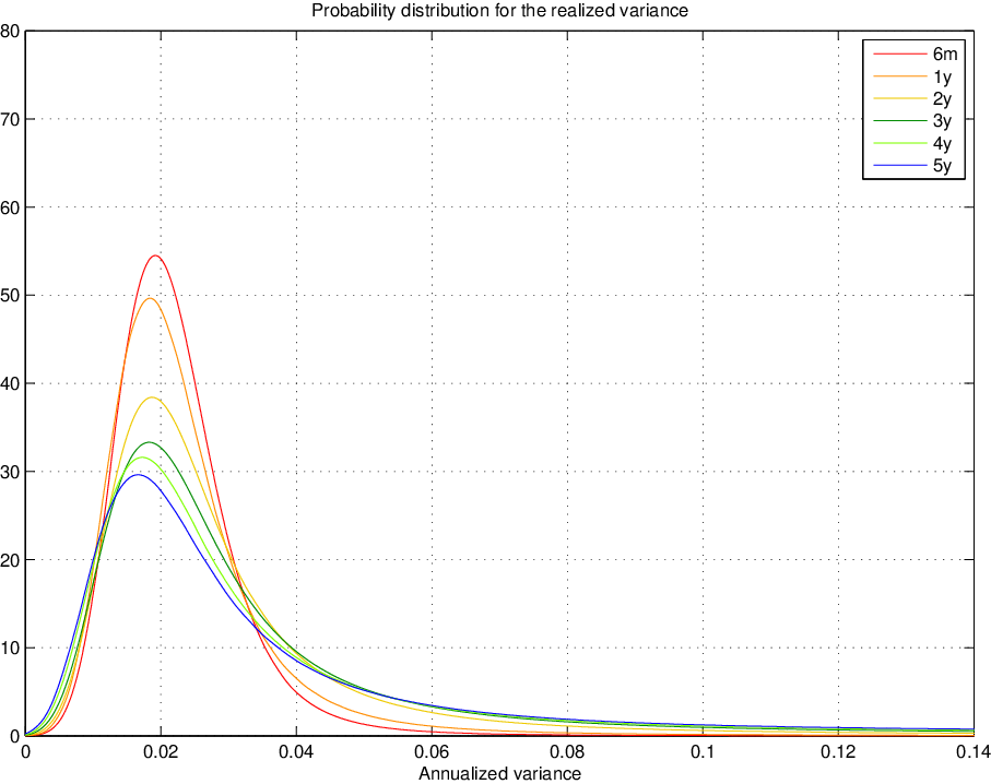