MCTP-09-14
Capture and Indirect Detection of Inelastic Dark Matter
Abstract
We compute the capture rate for Dark Matter in the Sun for models where the dominant interaction with nuclei is inelastic — the Dark Matter up-scatters to a nearby dark “partner” state with a small splitting of order a 100 keV. Such models have been shown to be compatible with DAMA/LIBRA data, as well as data from all other direct detection experiments. The kinematics of inelastic Dark Matter ensures that the dominant contribution to capture occurs from scattering off of iron. We give a prediction for neutrino rates for current and future neutrino telescopes based on the results from current direct detection experiments. Current bounds from Super–Kamiokande and IceCube-22 significantly constrain these models, assuming annihilations are into two-body Standard Model final states, such as , , or . Annihilations into first and second generation quarks and leptons are generally allowed, as are annihilations into new force carriers which decay dominantly into , and .
I Introduction
Detection of dark matter is one of the most important - and challenging - tasks of modern astrophysics. A wide range of experiments have been undertaken to search for this dark matter directly and indirectly. Of the direct detection experiments, which hope to find the recoil of a Weakly Interacting Massive Particle (WIMP), the signature is the recoil of a nucleus after collision with a dark matter particle. The key task in these experiments is the distinction between the rare event (a WIMP scatter) and the common background (arising from natural radioactivity or cosmic rays).
One approach is to take advantage of the motion of the Earth relative to the rotation of the Milky Way spiral arms. As the Earth revolves around the sun, the WIMPs generally scatter more frequently in underground detectors when the orbit of the Earth moves it into the DM “wind” that arises from the galactic rotation from the (expectedly) non-rotating dark matter halo. This effect raises the possibility of searching for Dark Matter through an annual modulation signature [1, 2]. The DAMA/LIBRA experiment has released data that displays an unmistakable annual modulation, consistent with this Dark Matter interpretation [3]. If confirmed, this would give a valuable clue to the identity of the Dark Matter that makes up a quarter of the critical density of the Universe. In the simplest models of Dark Matter, however, the DAMA/LIBRA signal is inconsistent with the the lack of observation in other low–background nuclear experiments, in particular XENON [4] and CDMS [5].
However, this conclusion does not apply to all Dark Matter models. It is possible to make the DAMA/LIBRA observation consistent with other direct dark matter detection experiments if what is being observed is actually inelastic scattering [6] of the type
| (1) |
In this process, the nuclear recoil spectra is sensitive to the mass difference . Only WIMPs that have energies above the mass splitting can drive the up-scattering to the heavier state. For keV, the recoil spectrum is sensitive to the target nucleus, raising the possibility that the scattering rates might differ drastically between experiments. This class of models has been shown to be consistent with both the recent DAMA/LIBRA data, as well as limits from the low-background experiments [7], see also [8, 9]. Inelastic Dark Matter could arise from mixed sneutrinos [6, 10, 11] or from an SU(2)-doublet [10, 9]. It can also be incorporated into models that explain [12] the recent tantalizing excesses from the PAMELA [13] experiment, as well as an excess from INTEGRAL via the mechanism of Ref. [14]. Should this interpretation hold, both the positive result from DAMA and the null results from the other low-background experiments will have been crucial in pointing us towards the correct theory of Dark Matter.
Indirect detection of Dark Matter through the annihilation into neutrinos can put strong constraints on Dark Matter models. Determination of the neutrino rate requires knowledge of the Dark Matter annihilation rate in the Sun (or Earth) as well as the spectrum of the annihilation products. Typically, a neutrino signal is potentially observable when the annihilation rate is in equilibrium with the capture rate (see, e.g., [15]). This capture rate is determined by the interaction of the Dark Matter with nuclei. Thus, the annihilation rate in the Sun is very sensitive to the scattering cross section off nuclei. So, capture rates are tied closely to the observed rate at DAMA/LIBRA, and neutrinos from the Sun are an important probe of any mechanism that explains that signal. Because of the gravitational potential of the Sun, WIMP capture in the Sun differs in important (but calculable) ways from the scattering off detectors in the Earth.
In this work, we first discuss the capture rate for inelastic Dark Matter (iDM) in the Sun. We then discuss the number of upward through-going muon-events that might be seen at detectors. This depends on the final states of the annihilation of WIMPs. The annihilations produce Standard Model particles, which eventually decay to neutrinos, which then propagate from the Sun to the detectors on Earth. A preliminary estimate of neutrino rates was made in [6], but here we extend the work, taking full account of the form factors in the scatterings, a proper treatment of the velocity distribution, as well as full propagation of the neutrinos from the center of the sun to the Earth.
II Inelastic Capture rate for inelastic dark matter
The central question in determining the rates of neutrinos is generally the WIMP capture rate on the sun. As WIMPs annihilate, one ultimately reaches equilibrium between capture and annihilation, i.e., . Thus, the capture sets the upper bound, and often the expected signal of neutrinos from the sun. In this section we present analytical formulae for calculating the capture rate of inelastic dark matter in the Sun.
An inelastic WIMP of mass can only scatter off a nucleus of mass if its energy . We will show a generalization of the results of Refs. [16] and [17], that allows for a discussion of the capture of inelastic dark matter.
II.1 Kinematics of Inelastic WIMP scattering
The kinematics of inelastic scattering are quite different from that of elastic scattering. To have any possibility of scattering at all, the WIMP must satisfy the kinetic energy requirement
| (2) |
The consequences of this change are purely kinematical. I.e.,
| (3) |
but the allowed energy ranges for scattering can be quite different. In the rest frame of the nucleus, conservation of energy and momentum of the WIMP–nucleus scattering process implies a minimum and maximum amount of energy loss in such a collision:
| (4) | |||||
| (5) |
where
| (6) |
We use the parameter to make connection with Ref. [16], which uses . We use to avoid confusion with the reduced mass parameter. This definition of is twice that for in Ref. [16].
As a consequence, the total cross section for inelastic scattering is
| (7) |
We will typically define our cross sections in terms of , which is the cross section per nucleon in the elastic limit.
II.2 WIMP velocity distribution and flux
To compute the scattering rate of the WIMPs on the Sun, we must characterize the distribution of WIMP velocities incident on the Sun. We assume that the WIMPs have an isothermal speed distribution in their rest frame. However, this frame need not coincide with the rest frame of the Sun. In the Sun’s rest frame, we have:
| (8) |
where is the velocity dispersion, and
| (9) |
with is the speed of the Sun with respect to the WIMP rest frame. The normalization factor, is given by Ref. [18]:
| (10) |
where , and is the escape velocity. In the limit of this expression simplifies to .
We now wish to compute the flux distribution of WIMPs incident on the Sun. We begin by considering an imaginary surface bounding a region of radius about the Sun, which is large enough so that the gravitational field due to the Sun is negligible. For an infinitesimal region of area we choose a local coordinate system (see Fig. 1) so that
| (11) | |||||
| (12) |

Therefore the flux of WIMPs with velocity in the range through the infinitesimal area is
| (13) | |||||
If we make the approximation that , then the analysis simplifies considerably. As we will see, we do not expect this assumption to drastically affect the results. With this assumption is possible to do a straightforward integration over (and )
| (14) | |||||
Here, is the modified Bessel function, and is the WIMP number density. We now change variables to angular momentum per unit mass . Therefore
| (15) |
and the total flux of WIMPs becomes
| (16) | |||||
| (17) |
where in the last line we take the limit. Therefore as expected the flux of WIMPs in the forward direction is greater than that in the direction opposite to the velocity of the Sun.
II.3 Differential capture rate
Following the calculation in Ref. [16], the WIMP velocity at the some inside the Sun is
| (18) |
and the probability for the WIMP to scatter inside a shell of thickness at radius is
| (19) | |||||
| (20) |
Therefore the differential capture rate is a product of the flux times the probability to scatter:
| (21) | |||||
To arrive at this expression, we performed the integral from to . The step function imposes the constraint that the energy of the WIMP is sufficient for the collision to occur. Therefore we find
| (22) |
where
| (23) | |||||
| (24) |
where in the last line we have performed the integral over . Note that if we had not taken the limit, the upper limit of integration on the integral would have been both and dependent, greatly complicating the analysis. Generalizing the result in Eqn. (A5) of Ref. [16] we have
| (25) |
where , , and is the maximum nuclear recoil energy in the elastic case. is the form factor that accounts for the fact that at sufficiently high momentum transfer, scattering from the nucleus is no longer coherent. We have also defined
| (26) |
where is the nucleon mass and is the WIMP-nucleon scattering cross-section. are the relative proton and neutron couplings, which we take to be equal. The results for the differential capture rate in Eqns. (22)–(26) represent the main analytic result of this paper.
II.4 Inelastic dark matter capture and astrophysical uncertainties
In this section we discuss the implications of Eqn. (22) and the uncertainty in the capture rate due to the astrophysical uncertainties in , and the distribution of heavy nuclei in the Sun. We also consider the effect of changes in in Eqn. (25). The changes in the capture rate that result from varying these astrophysical and nuclear parameters give us an estimate of some of the systematic uncertainties in our calculation and an idea of the robustness of the current limits we discuss in Sec. IV.1. As a reference point, we use the values GeV/cm3 and cm2 throughout this section: a change in these values will just rescale the total capture rate. Also, as reminder, this value of is chosen because the inelastic cross-section needed to make the DAMA/LIBRA results compatible with direct detection experiments is of the same order of magnitude.
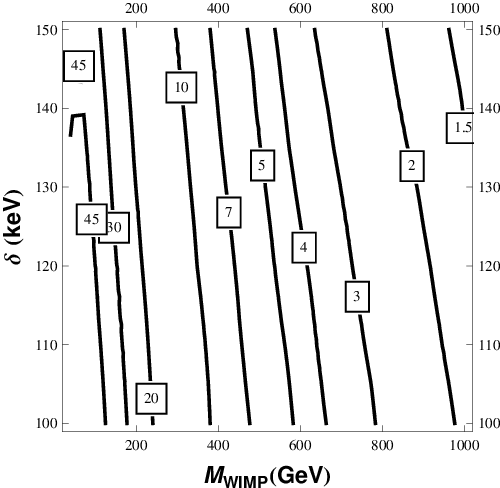
Before exploring the effects of these astrophysical uncertainties, we establish a baseline in Fig. 2. There we show the variation of the capture rate in the plane for the values km/s, and km/s. We have also used the Helm form factor from Ref. [18] for . As in the case of elastic dark matter, the capture rate decreases with increasing WIMP mass. This is in part due to a simple decrease in the number density of WIMPs. However, there are two additional effects: it is more difficult for heavy WIMPs to lose energy in collisions with the relatively light nuclei in the Sun, and as the mass of the WIMP increases, it becomes more difficult to satisfy the minimum scattering energy condition of Eqn. (2). The minimum scattering energy condition in Eqn. (2) leads to a suppression of the capture rate due to lighter nuclei, as shown in Fig. 3.


To focus on the effect that the inelasticity has on WIMP capture, in Fig. 3 we show the capture rate of a GeV WIMP on each species of nuclei in the Sun. We assume the same values of and as in Fig. 2. We see that for keV, the scattering of WIMPs off hydrogen and helium is highly suppressed, and in the range keV the capture due to scattering off iron dominates the other elements by a factor of. As a reminder, this range of values keV provides the best fit to the current DAMA data. The importance of the heavy elements for the capture rate is not unique to the inelastic case: for both elastic and inelastic (spin-independent) models scattering off the heaviest elements can dominate. (This is not true of spin-dependent scattering.) This is perhaps counter–intuitive, as the abundances of the heavy elements are substantially less than hydrogen and helium. However, these tiny abundances are compensated by the fact that the (coherent) spin-independent couplings scale as the square of the atomic number. In fact, when one accounts for additional kinematic factors, for large Dark Matter masses the spin-independent cross-section scales as the fourth power of the atomic mass number. These factors can more than overcome the relative scarcity of heavy elements. Some reviews in the literature dangerously neglect the contributions of these heavy elements for simplicity.
Depending on the choice of , there is actually a slight enhancement of capture due to iron relative to the elastic case. The reason is that form factor suppression is smaller for the inelastic case compared to the elastic one: for the same loss in WIMP energy the recoil energy of the nucleus is for the inelastic scenario compared to for WIMPs that scatter elastically. The net effect of inelastic scattering compared to the elastic case is shown in Fig. 4.


We now turn to sources of uncertainty in the capture rate. The importance of heavy nuclei in the capture of inelastic WIMPs implies a sensitivity to the abundance and distribution of these nuclei in the Sun, which is somewhat uncertain. To quantify this dependence on the distribution of heavy nuclei in the Sun we consider two variations to the Standard Solar Model of Ref. [19, 20]: a uniform distribution as a function of radius for all heavy nuclei and a linearly decreasing distribution with the same average number density as the uniform one (which we view as somewhat of an extreme case). We show these distributions, along with the resulting capture rates in Fig. 5. Again, we have set keV and values of and that are the same as those in Fig. 2. From Fig. 5 we see that if the number density of heavy nuclei in the center of the Sun is increased the overall capture rate can be significantly increased. Also, the mass fraction of iron in the Sun will directly affect the capture rate.

The threshold for scattering in Eqn. (2) also suggests that the capture rate is sensitive to variations in the astrophysical inputs and , as well as perhaps the escape velocity. First, we address the issue of the finite escape velocity. We do not expect the capture rate to be very sensitive to this quantity. This is because the particles that are most easily captured are not those particles in the Boltzmann tail. These particles have the most energy and are harder to capture. This is in strict contrast to scattering at DAMA/LIBRA, where only the most energetic particles in the Dark Matter distribution are able to drive the inelastic transition, simply because these particles do not have the benefit of mining the gravitiational potential energy of the Sun. (The intuition that the result is insensitive to was crudely confirmed by varying the (large) limit of the integral when performing the numerical integration, and seeing that the capture rate was insensitive.) In Fig. 6 we show the predicted range of values km/s with a central value of km/s in the red (solid) band and km/s with a central value of km/s in the blue (dashed) band, where we have used the Standard Solar Model heavy nuclei number densities, GeV/cm3and cm2. If one assumes no co-rotation of the WIMP halo, then the velocity of the Sun relative to the WIMP halo is determined as with km/s [21]. Recent measurements place km/s. We take this as a central value, but allow a range values to account for the possibility of errors in its determination and some co/counter-rotation. If one further assumes that the halo is virialized then , but we allow and to vary independently in the plot.
The variation in the capture rate illustrated in Fig. 6 is mainly due to the fact that mostly only slow moving WIMPs can lose sufficient energy to be captured. This effect dominates that of the WIMP minimum energy scattering condition in Eqn. (2). Therefore increasing has the effect of decreasing the capture rate. This result is the same as that observed in Refs. [16] and [17]. Even varying over this generous range, only a factor of two change in the capture rate is observed.
Finally, we note the importance of form factors to the discussion at hand. Due to the energy threshold in Eqn. (2) the WIMPs undergoing capture are relatively energetic and have to transfer a substantial portion of their energy to the nuclei. Therefore the recoil energy of the nuclei is large, and the process is very sensitive to the form factors used. If the Helm form factor overestimates the suppression for iodine at DAMA relative to iron for capture, it is possible that a relative factor of O(1) could result.
All together the uncertainties in astrophysical and nuclear inputs could lead to a factor of a few in the uncertainty of the capture rate of WIMPs in the Sun. The DAMA/LIBRA modulation signal is much more sensitive to the velocity distribution of the Dark Matter particles, on the other hand. This is because scatterings there only arise from particles in the tail of the velocity distribution. It is encouraging that the results for capture presented here are so robust.
III Capture vs. Annihilation in the Sun
We now review the interplay between capture and annihilation in the Sun. When the capture and annihilation rates are sufficiently large then equilibrium will be reached between the two processes.
Unless otherwise stated, we will assume that the capture and annihilation rates are sufficiently large so that the WIMPs are in equilibrium, and thus the annihilation rate is just one-half the capture rate: .
III.1 Thermalization in Elastic Models
A potentially major difference between the inelastic picture and the conventional picture is the question of what happens to WIMPs once they have scattered the first time and been trapped in the Sun. For conventional WIMPs, repeated scatters cause the WIMP to settle into thermal equilibrium in the center of the Sun. In contrast, for an inelastic WIMP, if the kinetic energy is suitably low, it is possible that no subsequent inelastic scatterings can take place. We must consider what occurs under these circumstances as well.
Let us begin by assuming that there are only inelastic scatterings. In this case, the WIMP will proceed through the Sun, scattering off iron (which is abundant at the 10-3 level), until such a point as it has insufficient kinetic energy to scatter off iron. There will be a range of orbits of varying ellipticity. Some will be circular, but most will be elliptical, and thus proceed more deeply into the Sun during their orbits. To determine how extensive this set of orbits will be, we must consider how much kinetic energy a given WIMP will have in the interior of the Sun.
A WIMP starting at rest from the surface of the Sun will have a velocity of approximately 1240 km/s in the center of the Sun. This is more than enough kinetic energy to scatter off iron for the parameters of interest. In fact, using the density profile in the solar models of [19, 20], simply going from to the center will give enough energy to inelastically scatter off iron. Thus, most WIMPs will be contained within this region.
We can now estimate whether the density in this region will be high enough to bring the system into equilibrium (i.e., the outgoing annihilation rate equals the capture rate). If we assume a capture rate , then (neglecting annihilation) the total number of particles in the Sun is , where is the age of the Sun. If the WIMPs are captured within a radius , the present annihilation rate is then
| (27) |
The annihilation will reach equilibrium with the capture if
| (28) |
The thermal cross section needed to produce the correct relic abundance () is sufficent to put the WIMPs into equilbrium unless it decreases with velocity (e.g. is p–wave). Should the WIMPs fail to reach equilibrium, there is an approximate overall suppression of the annihilation rate given by the LHS divided by the RHS. Note that even in models where a p-wave cross section determines the relic abundance, there is also a subdominant s-wave cross section. This s-wave scattering could well be sufficient to put the WIMPs in equilibrium.
Up to this point, we have considered particles with only inelastic scatterings, but (sub-dominant) elastic scatterings are common in many explicit models of inelastic Dark Matter. For instance, mixed sneutrino and neutrino models have sizable Higgs mediated couplings [6] ( cm2). Higgsinos–like models have loop-mediated contributions which can be important [22] ( cm2). Generically, inelastic models will have cross sections which are cm2 [10]. So how large a cross section is needed to thermalize?
The total number of scatters in the Sun over the age of the Sun for a WIMP would be
| (29) |
where is the typical density seen by the WIMP and is the proton mass. The solar density in the core is typically kg m-3, roughly 100 times larger than the mean solar density. To thermalize via scatterings off of protons, the WIMP must scatter of order times. Thus, a trapped 500 GeV WIMP scattering in the interior (with high densities) would need a cross section of approximately 10-48 cm2 to thermalize.
Models with light mediators typically will not have this, but they often have the Sommerfeld enhancement to boost annihilation rates to equilibrium. Models that are not pure SU(2) doublets, but instead have some mixing with SU(2) singlets after EWSB generally have large enough Higgs couplings. Finally, models which are pure SU(2) doublets - without Higgs couplings - generally have large enough loop induced cross sections to thermalize them in the core, although this is marginal for WIMPs much heavier than 500 GeV.
Thus, we believe even in the inelastic case, it is reasonable to generally consider models that annihilate in equilibrium with their capture rates. We will make this assumption in what follows.
IV Neutrino Rates
Armed with a capture rate, we can now predict the high energy neutrino flux (and the resulting muon rates) on the Earth. These rates will depend on the products of the WIMP annihilations. We considered the final states of , , , , , , and light jets. We will not explicitly show separate results for and as they are very similar.
If WIMP annihilations are solely to charged leptons of the first two generations the annihilation products interact strongly enough in the Sun that they typically come to rest before producing neutrinos. The neutrinos from such decays are low energy, and will not give an observable signal. A similar statement is true for particles that annihilate to first two generation/gluon jets. The neutrino production comes from fragmentation to heavy quarks, and is very suppressed. For our numerical results, we follow the work of Ref. [23], which builds on the work of Ref. [24].
IV.1 Existing Limits
Over the region of interest, the strongest bounds are placed by the Super-Kamiokande experiment [25] and the recent data from IceCube-22 [26]. At present, the limits are calculated assuming specific annihilation channels, which complicates the extraction of limits for a new model.
To place limits on the model at hand using the data from Super-Kamiokande, we calculate the number of expected signal events at the detector, following the methods of Ref. [27]. We first compute the flux of neutrinos from the Sun based on the appropriate annihilation channel.
We then propagate the neutrinos from the center of the Sun to the Earth, using the formula of Ref. [23] which are available at Ref. [28]. These results for propagation are consistent with those of Ref. [29]. From this neutrino flux, we calculate the rate of muons at Super-Kamiokande by using the formula
| (30) |
The muon effective area m2, and the livetime, , is given by days (the one-half is to account for night-time). The muon range, , is approximately given by
| (31) |
where is the relevant density, MeV cm2 g-1. varies depending on the material. For standard rock, cm2 g-1, whereas for water, cm2 g-1. At Super–K, there can be conversions both in the nearby rock and in the water. For simplicity, we will use the value cm2 g-1, as rock usually dominates. If we instead use the value for water the event rate increases by roughly 30. To compute the number events in Eqn. (30) we use the following neutrino-proton and neutrino-neutron cross-sections [30]:
| (32) | |||||
| (33) |
Here , , , , and the corresponding expressions for anti-neutrinos can be found by , , , .
The results from Eqn. (30) can then be compared to the data for upward going muons coming from the Sun as reported in [25]. To calculate the number of observed () and expected background () events as a function of the WIMP mass we use data on upward going muons from Fig.5 of Ref. [25]. The region of the sky surrounding the sun used in the search varies as a function of WIMP mass. We use Fig.8 of Ref. [31] to specify the angle about the sun that Sun as a function of the dark matter mass. through going muons is to Wimp annihilations in the Sun as a function
| (34) |
where the factor of takes into account the fact that only 90 % of the signal is contained with the window angle in Fig.8 of Ref. [31]. Therefore the maximum allowed number of events is the value needed so that the cumulative poisson distribution function is 10%, for number of observed events and number of expected events. The breaks in the curve around 90 and 225 GeV correspond to places where the size of the cone around the sun changes. In that cones size, there is a fluctuation in the number of events observed, which affects the limit. Note that the optimal cone size should actually depend on annihlation channel, as the neutrino spectra (and hence the correlation with direction) change with final state. However, the cone size in [31] is calculated instead with a ‘‘breadbasket’’ final states11 1 They take a final state of 80% , 10% and 10% ., so there is some uncertainty on the exact position of the curves.
If the Dark Matter annihilates to a hard channel (e.g., W bosons, top quarks or tau leptons) then the limits from Super–K are very constraining. For cross sections consistent with the DAMA result, the typical event rates at Super–K would be too large by some two orders of magnitude (see Fig. 7). If, instead the Dark Matter annihilates to a softer channel (bottom quarks or charm quarks), then the tension is lessened.
Nevertheless, it is fair to say that even in the case where the Dark Matter annihilates through a relatively soft channel such as charm (or more so with bottom quarks), there is tension with the existing limits from Super–Kamiokande. At larger masses, the inelastic explanation for DAMA comes into tension with results from the CDMS experiment [32]. However, N-body simulations have found significant structure in the high-velocity tails of velocity distributions [33], and these may open the ranges of parameter space significantly when included [34].


It is important to note bounds from some channels (e.g. tau leptons) are much stronger than those from others (e.g. b quarks). The result is that the dominant annihilation mode may not provide the most stringent bound on a given Dark Matter candidate. The plots in Fig. 7 can be used to extract the maximum branching ratio to a given channel.
Note, however, that at higher WIMP masses, (and especially for hard annihilation channels) the strongest limits come from the recent results of the 22-string run at IceCube. In Ref. [26], the collaboration quotes the maximum allowed values of the solar annihilation rate (= one-half capture rate in equilibrium) as a function of the neutralino mass for two different annihilation modes: (soft) and (hard). For the annihilation mode, IceCube-22 excludes capture rates above ( s-1) for GeV. No limits are quoted below 250 GeV. Comparing these rates with the capture rates of the previous section, we can see that these limits are very strong. For the softer annihilation channel, the limits are weaker: s-1 for GeV. No constraints on lower masses for soft channels are given. For reference, at 500 (250) GeV, a typical capture rate (for cm2) is s-1. Thus for quarks, the IceCube constraint on the cross-section is roughly comparable to that of Super-Kamiokande for masses greater than 500 GeV (see Fig. 8). Because of the large energy threshold at IceCube-22, it is dangerous to extrapolate to lower masses, or to draw a strong conclusion about annihilation to charm quarks. It is likely that IceCube should be able to probe these modes soon for higher masses (see next section).
For annihilation to bosons, IceCube-22 gives a bound that is nearly a factor of 4 stronger than Super-Kamiokande for masses greater than 250 GeV. Again, it is dangerous to extrapolate to lower masses. Something similar would be expected from other hard annihilation channels (tau leptons, top quarks, Z bosons). It is clear that IceCube-22 places strong constraints on the hard annihilation channels.
IV.2 Future Telescopes
We now turn to the sensitivity of future neutrino detection experiments to neutrino signals. We concentrate on the case of the IceCube experiment. We calculate both the expected number of events induced by neutrinos in the detectors, and the expected backgrounds that arise from the flux of atmospheric neutrinos.
For the atmospheric neutrino backgrounds, we use the data from Ref. [35] to derive a power law fit, which takes the approximate form
| (35) |
An experiment can focus only on the direction of the Sun to significantly reduce this background. We integrate over a 3∘ region for IceCube.
To calculate the actual number of events at IceCube, we again use Eqn. (30). For the purposes of determining the energy loss in ice, we take MeV cm2 g-1 and cm2 g-1. We take a threshold energy of GeV, which is somewhat optimistic but may be attainable, especially with the planned inclusion of the of the DeepCore array [36]. We take the effective area for IceCube from Ref. [37]. We find approximately 40 background events arising form atmospheric neutrinos within a window. The corresponding number of signal events, normalized to a cross section cm2 are shown in Fig. 9.


If nature has chosen the past of inelastic Dark Matter, perhaps the mostly likely reason that it has gone undetected thus far is annihilation proceeds to modes that provide soft neutrinos. Thus, it will be important for IceCube (and other future experiments such as ANTARES) to try and push their energy threshold as low as possible.
V Conclusions
Inelastic dark matter provides an exciting proposal to reconcile the results of DAMA/LIBRA with other direct detection experiments. However, its large cross section makes detection through neutrino telescopes a particularly important constraint. We have found that these experiments can place strong limits on these models, and so it is important to clearly state what those constraints are.
Under the assumption that inelastic dark matter s-wave annihilates with a thermal cross section, it certainly appears that for hard annihilation channels (e.g. tau leptons, W bosons, monochromatic neutrinos) such a scenario is excluded. For other cases where the annihilation products are softer sources of neutrinos (charm quarks or b quarks), the answer is less clear. Annihilation to charm, as well as other light quarks seems safe, at least within astrophysical uncertainties (though the tension in the charm channel is large at larger masses). Annihilation into b quarks seems excluded at the factor of two level (and more for higher masses). When including the variety of uncertainties, both from astrophysics as well as other issues such as nuclear form factors this is borderline. It is important to note, however, that annihilations into Higgs bosons generally include a component of as well, which even as subdominant contributions are often the dominant limit. In particular when considering the IceCube-22 limits, particles above GeV are strongly constrained.
We should note that these limits are possibly evaded in elastic models when the annihilation rate is p-wave suppressed, and equilibrium between annihilation and capture has not yet been achieved.
Importantly, models in which the dark matter annihilates into new, light force carriers that dominantly decay into , and appear safe from these constraints, because muons and pions stop before decaying and producing neutrinos.
Another possibility to evade these bounds is that the Dark Matter might dominantly annihilate to large multiplicity final states. In this case, the neutrino energies are degraded, as the energy is shared amongst a large number of final decay products, and limits might easily be evaded. This could occur naturally in light mediator models, where one might have , or models where the Higgs boson dominantly decays via pseudo-scalars [38], in which case . If the light states ( or ) are allowed to decay to leptons or directly to neutrinos, then tension may still exist. A detailed examination of such decays and related model building is left for future work[39]. Because the bounds on the channels with energetic neutrinos are so much stronger, it is possible (or even likely) that a sub-dominant decay mode with hard neutrinos could provide the strongest constraint for models of this type. This is also of potential relevance if Higgs boson decays are involved and both leptons and -quarks are potentially present.
In the case where Dark Matter is not its own anti-particle, and possesses a conserved quantum number, the Dark Matter abundance is due to a small excess of Dark Matter over anti–Dark Matter. Then captured Dark Matter may not annihilate and there will be no signal. Such a scenario is incompatible with potential annihilation signals observed by PAMELA and FGST.
Ultimately, the space of models to explain DAMA through inelastic scattering is still large, but the space is strongly constrained by these neutrino telescopes. Should future direct detection bear out the presence of inelastic WIMPs, particularly at higher masses, these null results should allow us to distinguish among a variety of candidates.
Acknowledgements.
We would like to thank Patrick Fox, Dan Hooper, Michele Papucci, and Chris Savage for useful discussions, and Itay Yavin for many helpful discussions and informing us of his work[40]. The authors also thank Carlos Peña-Garay for providing us with detailed information about solar elemental distributions. The work of A. Menon and A. Pierce is supported under DOE Grant #DE-FG02-95ER40899. The work of A. Pierce is also supported by NSF CAREER Grant NSF-PHY-0743315. The work of R. Morris and N. Weiner is supported by NSF CAREER grant PHY-0449818 and DOE OJI grant #DE-FG02-06ER41417.References
- [1] A. K. Drukier, K. Freese, and D. N. Spergel, Phys. Rev. D33, 3495 (1986).
- [2] K. Freese, J. A. Frieman, and A. Gould, Phys. Rev. D37, 3388 (1988).
- [3] R. Bernabei et al. (DAMA), Eur. Phys. J. C56, 333 (2008), eprint 0804.2741.
- [4] J. Angle et al. (XENON), Phys. Rev. Lett. 100, 021303 (2008), eprint 0706.0039.
- [5] D. S. Akerib et al. (CDMS), Phys. Rev. Lett. 96, 011302 (2006), eprint astro-ph/0509259.
- [6] D. Tucker-Smith and N. Weiner, Phys. Rev. D64, 043502 (2001), eprint hep-ph/0101138.
- [7] S. Chang, G. D. Kribs, D. Tucker-Smith, and N. Weiner (2008a), eprint 0807.2250.
- [8] J. March-Russell, C. McCabe, and M. McCullough (2008a), eprint 0812.1931.
- [9] Y. Cui, D. E. Morrissey, D. Poland, and L. Randall (2009), eprint 0901.0557.
- [10] D. Tucker-Smith and N. Weiner, Phys. Rev. D72, 063509 (2005), eprint hep-ph/0402065.
- [11] Z. Thomas, D. Tucker-Smith, and N. Weiner, Phys. Rev. D77, 115015 (2008), eprint 0712.4146.
- [12] N. Arkani-Hamed, D. P. Finkbeiner, T. R. Slatyer, and N. Weiner, Phys. Rev. D79, 015014 (2009), eprint 0810.0713.
- [13] O. Adriani et al. (PAMELA), Nature 458, 607 (2009), eprint 0810.4995.
- [14] D. P. Finkbeiner and N. Weiner, Phys. Rev. D76, 083519 (2007), eprint astro-ph/0702587.
- [15] G. Jungman, M. Kamionkowski, and K. Griest, Phys. Rept. 267, 195 (1996), eprint hep-ph/9506380.
- [16] A. Gould, Astrophys. J. 321, 571 (1987).
- [17] A. Gould, Astrophys. J. 388, 338 (1992).
- [18] J. D. Lewin and P. F. Smith, Astropart. Phys. 6, 87 (1996).
- [19] J. N. Bahcall, A. M. Serenelli, and S. Basu, Astrophys. J. 621, L85 (2005), eprint astro-ph/0412440.
- [20] C. Pena-Garay and A. Serenelli (2008), eprint 0811.2424.
- [21] W. Dehnen and J. Binney, Mon. Not. Roy. Astron. Soc. 298, 387 (1998), eprint astro-ph/9710077.
- [22] J. Hisano, S. Matsumoto, M. M. Nojiri, and O. Saito, Phys. Rev. D71, 015007 (2005), eprint hep-ph/0407168.
- [23] M. Cirelli et al., Nucl. Phys. B727, 99 (2005), eprint hep-ph/0506298.
- [24] G. Jungman and M. Kamionkowski, Phys. Rev. D51, 328 (1995), eprint hep-ph/9407351.
- [25] S. Desai et al. (Super-Kamiokande), Phys. Rev. D70, 083523 (2004), eprint hep-ex/0404025.
- [26] R. Abbasi (2009), eprint 0902.2460.
- [27] C. Delaunay, P. J. Fox, and G. Perez (2008), eprint 0812.3331.
- [28] http://www.marcocirelli.net/DMnu.html.
- [29] M. Blennow, J. Edsjo, and T. Ohlsson, Phys. Scripta T127, 19 (2006).
- [30] V. Barger, W.-Y. Keung, G. Shaughnessy, and A. Tregre, Phys. Rev. D76, 095008 (2007), eprint 0708.1325.
- [31] M. Mori et al. (KAMIOKANDE), Phys. Rev. D48, 5505 (1993).
- [32] J. March-Russell, C. McCabe, and M. McCullough (2008b), eprint 0812.1931.
- [33] M. Vogelsberger et al. (2008), eprint 0812.0362.
- [34] M. Kuhlen and N. Weiner (2009).
- [35] M. Honda, T. Kajita, K. Kasahara, S. Midorikawa, and T. Sanuki, Phys. Rev. D75, 043006 (2007), eprint astro-ph/0611418.
- [36] E. Resconi and f. t. I. Collaboration, Nucl. Instrum. Meth. A602, 7 (2009), eprint 0807.3891.
- [37] M. C. Gonzalez-Garcia, F. Halzen, and M. Maltoni, Phys. Rev. D71, 093010 (2005), eprint hep-ph/0502223.
- [38] S. Chang, R. Dermisek, J. F. Gunion, and N. Weiner, Ann. Rev. Nucl. Part. Sci. 58, 75 (2008b), eprint 0801.4554.
- [39] A. Menon, A. Pierce, and N. Weiner, in preparation.
- [40] S. Nussinov, L. Wang, and I. Yavin (2009), eprint 0905.1333 (hep-ph).