Anomalous behavior of trapping on a fractal scale-free network
Random walks and Levy flights Networks and genealogical trees Classical transport
Anomalous behavior of trapping on a fractal scale-free network
Abstract
It is known that the heterogeneity of scale-free networks helps enhancing the efficiency of trapping processes performed on them. In this paper, we show that transport efficiency is much lower in a fractal scale-free network than in non-fractal networks. To this end, we examine a simple random walk with a fixed trap at a given position on a fractal scale-free network. We calculate analytically the mean first-passage time (MFPT) as a measure of the efficiency for the trapping process, and obtain a closed-form expression for MFPT, which agrees with direct numerical calculations. We find that, in the limit of a large network order , the MFPT behaves superlinearly as with an exponent much larger than 1, which is in sharp contrast to the scaling with , previously obtained for non-fractal scale-free networks. Our results indicate that the degree distribution of scale-free networks is not sufficient to characterize trapping processes taking place on them. Since various real-world networks are simultaneously scale-free and fractal, our results may shed light on the understanding of trapping processes running on real-life systems.
pacs
05.40.Fbpacs
89.75.Hcpacs
05.60.Cd1 Introduction
In the past decade, there has been a considerable interest in characterizing and understanding the structural properties of networked systems [1]. It has been established that scale-free behavior [2] is one of the most fundamental concepts for a basic understanding of the organization of many real-world systems in nature and society. This scale-free property has a profound effect on almost every aspect on dynamic processes taking place on networks [3], including robustness [4], percolation [5, 6], synchronization [7], games [8], epidemic spreading [9], to name just a few. For instance, for a wide range of scale-free networks an epidemic threshold does not exist, and even infections with a low spreading rate will prevail over the entire population in these networks [9]. This is a radical change from the conclusions drawn from classical disease modeling [10].
In addition to the above-mentioned dynamics, some authors have focused their attention on the trapping problem occurring on complex networks [11, 12, 13, 14, 15, 16, 17], which is one of the main topic of interest for random walks (diffusion) [18, 19]. The classical trapping problem first introduced in [20] is a random-walk issue, where a trap is located at a fixed position, absorbing all particles that visit it. An interesting quantity closely related to the trapping problem is the mean first-passage time (MFPT), which is very important in the study of transport-limited reactions [21, 22], and target search [23, 24], amongst other physical problems. A result from previous research is that a power-law property can improve the efficiency of transport by diffusion on scale-free networks [11, 15, 16, 17]: the MFPT, , scales linearly or sublinearly with the number of network nodes as with or , which shows that the efficiency of trapping processes on scale-free networks is even better than (at least not worse than) that on complete graphs [11], the best possible structure for a fast diffusion (with ).
Although the scale-free topology has a direct effect on other structural characteristics (e.g., average path length [25]) of networks and dynamics running on them, it cannot reflect all the information of the network structure. Recently, it has been discovered that many real-life networks, such as the WWW, metabolic networks, and yeast protein interaction networks have self-similar properties and exhibit fractal scaling [26, 27, 28]. This fractal topology is often characterized through the fractal dimension , which can be obtained by the box-counting algorithm [29, 30]. It is now commonly accepted that fractal scaling [26] must be considered in an integral basic understanding of the organization of real-life complex systems.
As a fundamental property, topological fractality is related to many respects of network structure and function. Recently, several authors have shown that the correlation between degree and betweenness centrality of nodes is much weaker in fractal network models in comparison with non-fractal models [31, 32]. It has been also shown [27, 33] that fractal scale-free networks are disassortative [34], and this feature, together with fractality, makes such scale-free networks more robust against intentional attacks on hub nodes, as compared to the highly vulnerable non-fractal scale-free networks [27]. In addition to the distinction in the robustness, fractal networks exhibit lower synchronizability than their non-fractal counterparts [33]. Although a lot of efforts have been devoted to fractal scale-free networks [35, 36, 37, 38, 39], it is still of current interest to look for a better understanding of the consequences of a fractal topology on different dynamic processes.
In this paper, we study the trapping dynamics on a fractal scale-free network in the presence of a perfect absorber located at a fixed node. We obtain a rigorous solution for the MFPT of the unbiased random walks, which is computed through the recurrence relations derived from the network structure. The resulting formula shows that for a large network, the MFPT, , scales with the network order as . This superlinear growth is significantly different from the linear or sublinear scaling previously found for nonfractal scale-free networks.
2 The fractal scale-free network
In this section we introduce a network model defined in an iterative way [27], which has attracted a great amount of attention [12, 36, 32, 40]. We call this model iterative fractal scale-free tree (IFSFT). We study the IFSFT because of its intrinsic interest and its relevance to real-world systems. For example, the so-called border tree motifs have been shown to be present, in a significant way, in real-life networks [41]. Moreover, the IFSFT is deterministic, which allows us to study analytically its topological properties and dynamical processes taking place on it. It is thus a good test-bed and an ideal substrate network.
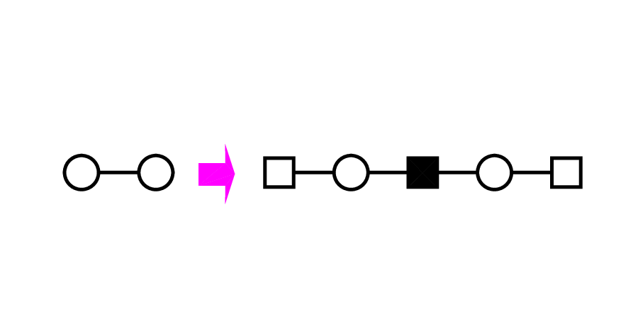
The IFSFT, denoted by after () iterations (the number of iterations is also called generation hereafter), is constructed as follows. For , is an edge connecting two nodes. For , is obtained from : for each edges in , two new nodes (called external nodes with degree of 1) are firstly introduced and linked respectively to both ends of the edge; then, the edge is broken, another new node (referred to as an internal node) is positioned in its middle and connected to both ends (see Fig. 1). In other words, is obtained from by performing the following operations on every edge in : replace the edge by a path of 2 links long, with the two endpoints of the path being the same endpoints of the original edge, then attach a new node to each endpoint of the path. Figure 2 shows the construction process for the first three iterative processes.

According to the network construction, one can see that at each generation () the number of newly introduced nodes is . From this result, we can easily compute the network order (i.e., the total number of nodes) at generation :
| (1) |
To facilitate the description in what follows, we distinguish different nodes of by labeling them as follows. For , the newly created internal node is labeled 1, the initial two nodes belonging to are labeled as 2 and 3, and the two new external nodes have labels 4 and 5, see Fig. 3. For each new iteration , we label consecutively the new nodes generated at this iteration, while we keep the labels of the old nodes unchanged. Namely, new nodes are labeled sequentially as . In this way, we label each node by a unique integer: at generation all nodes are labeled from 1 to .

Let be the degree of a node at generation , which entered the network at generation (). If node was an external node when it was introduced,
| (2) |
otherwise, if was an internal node when it entered the network,
| (3) |
From Eqs. (2) and (3), one can easily see that after each new iteration the degree of a node doubles, i.e.,
| (4) |
The IFSFT presents some interesting topological characteristics. It has a power law degree distribution with exponent [36, 32]. Its average path length, defined as the mean of shortest distances between all pairs of nodes, grows as a square power of the network order [32]. The betweenness distribution of its nodes exhibits a power-law behavior with exponent [32]. Particulary, it is fractal with the fractal dimension .
After introducing the IFSFT, in what follows we will study the MFPT for random walks with a single immobile trap on the network. We will show that the fractal property has an essential influence on the MFPT, i.e., the fractality can induce a general slowing down of diffusion.
3 Formulation of trapping problem on the IFSFT
Here we formulate the trapping problem of a simple random walk of a particle on the IFSFT in the presence of an absorbing trap positioned at the central hub node , represented as . To this end, we first represent by its adjacency matrix of order . The entry of is either 1 or 0: if and are adjacent and otherwise. The diagonal degree matrix of is . Then, the normalized Laplacian matrix of is given by , where is the identity matrix.
In the trapping problem, at each time step, a particle, starting from any node except the trap , moves from its current location to any of its nearest neighbors with equal probabilities. It is easy to see that in the end the particle will be necessarily absorbed by the trap, regardless of its starting location [11]. We are interested in the mean transmit time (first-passage time, or trapping time) for a particle, originating at node , to first reach the trap in .
Such a random walk can be described by a Markov chain [42], whose fundamental matrix is the inverse of matrix that is defined as a sub-matrix of the normalized Laplacian matrix obtained by deleting from it the first row and column, corresponding to the absorbing node. The entry of the fundamental matrix expresses the mean residence time, which is the mean number of visitations of node by the particle, starting from node , before trapping occurs. Thus, we have
| (5) |
Then, the MFPT, , which is the mean of over all nodes distributed uniformly over nodes in other than the trap, is given by
| (6) |
Equation (6) shows that the problem of finding is reduced to calculating the sum of all entries of the fundamental matrix . Although the expression of Eq. (6) seems compact, since the order, , of increases exponentially with , for large , it becomes impossible to get through direct calculation from Eq. (6) as we are restricted by time and computer memory, and one can calculate directly the MFPT only for the first iterations, see Fig. 4. However, the particular construction of the IFSFT and the special choice of the trap location allow to calculate analytically MFPT to obtain a closed-form formula. The derivation details of which will be provided in the following section.

4 Explicit expression for MFPT
Before giving a general formula for MFPT, , we first establish the dependence of on .
4.1 Evolution scaling for trapping time
For each , the values of can be obtained straightforwardly via Eq. (5). Table 1 lists the numerical values of for nodes for the first several generations up to . The numerical values quoted in table 1 show that for a given node we have . That is to say, upon growth of the IFSFT from generation to , the mean time to first reach the trap increases by a factor of 8. This is a basic characteristic of random walks on the IFSFT, which can be established from the arguments below.
Consider an arbitrary node in the IFSFT . From Eq. (4), we know that at iteration , the degree of node of IFSFT doubles, i.e., it grows from (degree at iteration ) to . Moreover, all these neighbors are new nodes created at iteration , among which neighbors are external nodes, and the rest neighbors are internal nodes. We now examine the standard random walk in : Let be the mean transmit time for a particle starting from node to any of its old neighbors, i.e., those nodes directly linked to node at iteration ; and let (resp. ) be the mean transmit time for going from any of the internal (resp. external) neighbors of to one of the old neighbors. Then the mean transmit times follow the relations:
Equation (4.1) has a solution , found by eliminating and . That is to say, when the network grows from iteration to iteration , the first-passage time from any node to any node (both and belong to ) increases by a factor of 8. Thus, we have , which will be useful for the derivation of the exact formula for the MFPT below.
| (2,3) | (4,5) | (6,7) | (8,9) | (10,11,12,13) | (14,15) | (16,17) | |
|---|---|---|---|---|---|---|---|
| 1 | |||||||
| 2 | |||||||
| 3 | |||||||
| 4 | |||||||
| 5 | |||||||
| 6 |
4.2 Formula for the MFPT
After obtaining the scaling of mean trapping time for old nodes, we now derive the analytical rigorous expression for the MFPT. Before proceeding further, we first introduce some notation used in the rest of this section. Let denote the set of nodes in , and let stand for the set of those nodes introduced at generation . To facilitate the computation, we also define the following quantities for :
| (11) |
and
| (12) |
By definition, it follows that . Thus, we have
| (13) |
where the relation of has been made use of. Hence, to determine , one should first explicitly determine the quantity . For this purpose, we further separate into two sets: one set of external nodes and the other set of internal nodes as defined in the second section, which are denoted as and , respectively. Clearly, . On the other hand, we have shown that the cardinality of set is , and that . Thus, we can obtain and . Then, two corresponding quantities can be defined:
| (14) |
| (15) |
It is obvious that
| (16) |

In order to obtain , one may alternatively get and . To this end, we first establish the relationship between the two quantities and . By construction, at a given generation, each edge connecting two nodes and (see Fig. 5) will generate three new nodes in the next generation: two external nodes ( and ) and one internal node (), and the mean transmit times for these three new nodes satisfy the following relations:
Hence, we have
| (21) |
Summing Eq. (21) over all old edges at the generation before growth, we can easily obtain that for all ,
| (22) |
Equation (22) gives the relationship between and , which is very significant since it is useful for the computation in the following text.
Therefore, the issue of determining is reduced to finding the quantity that can be obtained as follows. For an arbitrary external node in , which is created at generation and attached to an old node , we have
| (23) |
since a particle starting from node will be on node after one jump. Note that Eq. (23) holds for any node pair consisting of an old node and any one of its new external adjacent nodes. By applying Eq. (23) to two sum (the first one is over a given old node and all its new external nodes, the other is summing the first one over all old nodes), we get
| (24) | |||||
Now, we can determine through a recurrence relation, which can be obtained easily. From Eq. (24), it is not difficult to write out as
| (25) |
Equation (25) minus Eq. (24) times 16 and making use of the relation , one gets the following recurrence relation
| (26) |
Considering the initial condition , this recurrence relation is solved to obtain
| (27) |
Inserting Eq. (27) into Eq. (16) and considering the relation , we have
| (28) |
Substituting the last expression into Eq. (13) yields
| (29) |
Using , Eq. (29) is solved inductively
| (30) |
Inserting Eq. (30) into Eq. (6), we obtain the rigorous expression for the MFPT for the trapping problem on the -th generation of the IFSFT:
| (31) |
We have checked this exact solution for the MFPT against numerical values given by Eq. (6), see Fig. 4. For all , the analytical values obtained from Eq. (31) are perfectly consistent with the numerical results. This agreement is an independent test of our theoretical formula.
We show next how to represent MFPT as a function of the network order, with the aim of obtaining the relation between these two quantities. Recalling Eq. (1), we have and . Hence, Eq. (31) can be recast as
| (32) |
For a large network, i.e., ,
| (33) |
with the exponent much larger than 1. Thus, in the limit of large network order , the MFPT grows superlinearly with the number of network nodes.
Recently, it has been shown that for non-fractal scale-free networks with a large network order , their MFPT behaves linearly or sublinearly with as with [11, 15, 16, 17]. However, we have seen that for the IFSFN, the MFPT, , increases superlinearly with (i.e., ) irrespective of its scale-free property, presenting an obvious difference from the results previously obtained for its non-fractal scale-free counterparts.
Why is the MFPT for the IFSFT far larger than that for nonfractal scale-free networks such as the Apollonian network [16]? The reasons behind this discrepancy may be explained as follows. For the Apollonian network, the large-degree nodes, including the trap node, are directly connected to one another and compose a core group sharing more neighbors, which make the Apollonian network be a very compact system. So, these large-degree nodes can be easily visited by a particle in spite of its starting location. The interconnection within nodes with large degrees makes the particle spend a short time to find the trap. On the contrary, in the IFSFT, the large-degree nodes are not linked to each other, they are exclusively connected to low-degree nodes, as a result from the fractal property of IFSFT. In other words, there is an effective ‘repulsion’ between the large-degree nodes in the IFSFT [27, 32], which seems to be a main feature that distinguishes the IFSFT from the Apollonian network. Hence, for the trapping problem in the IFSFT, because of the isolation of the large-degree nodes from each other, the particle will first reach a hub node, and before being absorbed it will spend a lot of time in the intermediate regions constituted by small-degree nodes, which connect indirectly the large-degree nodes to one another. Therefore, it takes a longer time for the particle to arrive at the trap.
5 Conclusions
We have studied a classical trapping problem performed on a deterministically growing scale-free network with fractal topology. The self-similarity of the network allows us to derive the exact expression for the MFPT. We have shown that, for large networks, the MFPT increases as a power-law function of the network order, with an exponent much larger than 1, in contrast with previous results found for non-fractal scale-free networks. We see that this slow transport efficiency lies with the inherent fractality and its associated disassortativity. Thus, we can infer that scale-free networks do not always tend to accelerate the diffusion processes occurring on them. Our research may be helpful for a better understanding of the role that network structure plays in a trapping process.
6 Acknowledgment
We thank F. Comellas for his help in revising the manuscript. This research was supported by the National Basic Research Program of China under grant No. 2007CB310806, the National Natural Science Foundation of China under Grant Nos. 60704044, 60873040 and 60873070, Shanghai Leading Academic Discipline Project No. B114, and the Program for New Century Excellent Talents in University of China (NCET-06-0376). W L Xie also acknowledges the support provided by Hui-Chun Chin and Tsung-Dao Lee Chinese Undergraduate Research Endowment (CURE).
References
- [1] R. Albert and A.-L. Barabási, Rev. Mod. Phys. 74, 47 (2002).
- [2] A.-L. Barabási and R. Albert, Science 286, 509 (1999).
- [3] S. N. Dorogovtsev, A. V. Goltsev and J.F.F. Mendes, Rev. Mod. Phys. 80, 1275 (2008).
- [4] R. Albert, H. Jeong, A.-L. Barabási, Nature (London) 406, 378 (2000).
- [5] D. S. Callaway, M. E. J. Newman, S. H. Strogatz, and D. J. Watts, Phys. Rev. Lett. 85, 5468 (2000).
- [6] R. Cohen, K. Erez, D. ben-Avraham, and S. Havlin, Phys. Rev. Lett. 86, 3682 (2001).
- [7] A. Arenas, A. Díaz-Guilera, J. Kurths, Y. Moreno, and C. S. Zhou, Phy. Rep. 469, 93 (2008).
- [8] G. Szabó and G. Fáth, Phy. Rep. 446, 97 (2007).
- [9] R. Pastor-Satorras and A. Vespignani, Phys. Rev. Lett. 86, 3200 (2001).
- [10] H. W. Hethcote, SIAM Rev. 42, 599 (2000).
- [11] E. M. Bollt, D. ben-Avraham, New J. Phys. 7, 26 (2005).
- [12] S. Condamin, O. Bénichou, V. Tejedor, R. Voituriez, and J. Klafter, Nature (London) 450, 77 (2007).
- [13] A. Kittas, S. Carmi, S. Havlin, and P. Argyrakis, EPL 84, 40008 (2008).
- [14] A. G. Cantú and E. Abad, Phys. Rev. E 77, 031121 (2008).
- [15] Z. Z. Zhang, Y. C. Zhang, S. G. Zhou, M. Yin, and J. H. Guan, J. Math. Phys. 50, 033514 (2009).
- [16] Z. Z. Zhang, J. H. Guan, W. L. Xie, Y. Qi, and S. G. Zhou, EPL 86, 10006 (2009).
- [17] Z. Z. Zhang, Y. Qi, S. G. Zhou, W. L. Xie, and J. H. Guan, Phys. Rev. E 79, 021127 (2009).
- [18] S. Havlin and D. ben-Avraham, Adv. Phys. 36, 695 (1987).
- [19] R. Metzler and J. Klafter, J. Phys. A: Math. Gen. 37, R161 (2004).
- [20] E. W. Montroll, J. Math. Phys. 10, 753 (1969).
- [21] S. B. Yuste and K. Lindenberg, Chem. Phys. 284, 169 (2002).
- [22] C. Loverdo, O. Bénichou, M. Moreau, and R. Voituriez, Nature Phys. 4, 134 (2008).
- [23] O. Bénichou, M. Coppey, M. Moreau, P.-H. Suet, and R. Voituriez, Phys. Rev. Lett. 94, 198101 (2005).
- [24] M. F. Shlesinger, Nature (London) 443, 281 (2006).
- [25] R. Cohen and S. Havlin, Phys. Rev. Lett. 90, 058701 (2003).
- [26] C. Song, S. Havlin, H. A. Makse, Nature 433, 392 (2005).
- [27] C. Song, S. Havlin, H. A. Makse, Nature Phys. 2, 275 (2006).
- [28] K.-I. Goh, G. Salvi, B. Kahng and D Kim, Phys. Rev. Lett. 96, 018701 (2006).
- [29] C. Song, L. K. Gallos, S. Havlin, H. A. Makse, J. Stat. Mech.: Theory Exp. P03006, (2007).
- [30] L. Gao, Y. Q. Hu, and Z. R. Di, Phys. Rev. E 78, 046109 (2008).
- [31] M. Kitsak, S. Havlin, G. Paul, M. Riccaboni, F. Pammolli, and H. E. Stanley, Phys. Rev. E 75, 056115 (2007).
- [32] Z. Z. Zhang, S. G. Zhou, L. C. Chen, and J. H. Guan, Eur. Phys. J. B 64, 277 (2008).
- [33] Z. Z. Zhang, S. G. Zhou, and T. Zou, Eur. Phys. J. B 56, 259 (2007).
- [34] M. E. J. Newman, Phys. Rev. Lett. 89, 208701 (2002).
- [35] M. Hinczewski and A. N. Berker, Phys. Rev. E 73, 066126 (2006).
- [36] H. D. Rozenfeld, S. Havlin, and D. ben-Avraham, New J. Phys. 9, 175 (2007).
- [37] H. D. Rozenfeld and D. ben-Avraham, Phys. Rev. E 75, 061102 (2007).
- [38] M. Hinczewski, Phys. Rev. E 75, 061104 (2007).
- [39] Z. Z. Zhang, S. G. Zhou, T. Zou, and G. S. Chen, J. Stat. Mech.: Theory Exp. P09008 (2008).
- [40] L. K. Gallos, C. Song, S. Havlin, and H. A. Makse, Proc. Natl. Acad. Sci. USA 104, 7746 (2007).
- [41] P. Villas Boas, F. A. Rodrigues, G. Travieso, and L. Costa, J. Phys. A 41, 224005 (2008).
- [42] J. G. Kemeny and J. L. Snell, Finite Markov Chains (Springer, New York, 1976).