Dynamical self-stabilization of the Mott insulator Atoms in optical lattices Density functional theory, local density approximation Lattice fermion models (Hubbard model, etc.)
Dynamical self-stabilization of the Mott insulator: Time evolution of the density and entanglement entropy of out-of-equilibrium cold fermion gases
Abstract
The time evolution of the out-of-equilibrium Mott insulator is investigated numerically through calculations of space-time resolved density and entropy profiles resulting from the release of a gas of ultracold fermionic atoms from an optical trap. For adiabatic, moderate and sudden switching-off of the trapping potential, the out-of-equilibrium dynamics of the Mott insulator is found to differ profoundly from that of the band insulator and the metallic phase, displaying a self-induced stability that is robust within a wide range of densities, system sizes and interaction strengths. The connection between the entanglement entropy and changes of phase, known for equilibrium situations, is found to extend to the out-of-equilibrium regime. Finally, the relation between the system’s long time behavior and the thermalization limit is analyzed.
pacs
37.10.Jkpacs
71.15.Mbpacs
71.10.Fd1 Introduction
The experimental realization of ultracold gases of fermionic atoms in optical lattices is one of the major scientific breakthroughs of the past years [2, 3, 4]. The high tunability of parameters in optical lattices permits to study fermionic atoms with repulsive as well as attractive interactions [5]. These investigations reveal a multitude of scenarios which depend on the strength and the sign of the inter-particle interactions (for example, for the attractive case, at low temperatures, a complex phase diagram results, with several competing phases [6]).
In this paper, we will consider repulsive fermions. In addition to the Pauli exclusion principle, the physics of such systems is governed by three distinct energy scales: the kinetic energy of the fermions, the potential energy due to the confining trap potential, and the fermion-fermion interaction energy.
Various numerical [7, 8, 9, 10] and analytical [11] techniques predict that this interplay gives rise to a characteristic spatially varying density profile, displaying coexistence of metallic, Mott-insulator and band-insulator-like regions in different parts of the trap. Very recently, evidence for such phase-separated density profiles in three-dimensional fermion gases has been obtained experimentally [3, 10].
Most such investigations have been directed at stationary states, to make contact with possible ground states of strongly-correlated, many-electron, condensed-matter systems. Trapped fermions on an optical lattice, however, also allow one to study the time evolution of such systems, much more directly and easily than in solid-state experiments, and in great detail [12, 13, 14, 15, 16, 17]. Very recently, for example, experiments have probed possible metastable states of cold atom gases, and the possibility of a dynamical tuning of the lattice and interaction parameters [18]. In other work [19], self-induced shape-stability was observed for a expanding turbulent bosonic cloud.
Motivated by such experiments, we here study numerically the time evolution of the Mott insulator, band-insulator and metallic phases after rapid, moderate and adiabatic switching-off of the trapping potential. This allows us to address a fundamental question of many-body physics: How does the time evolution of a Mott insulator differ from that of a band insulator and of a metallic phase ?
Before describing our methods and results, we recall that in a completely different part of physics a similar shift from static to time-dependent (TD) investigations is taking place: the study of entanglement in many-body systems. Entanglement in such systems is commonly studied in connection to quantum criticality, where a deep connection between extrema of the entanglement entropy (EE) and quantum-phase transitions was found [20, 21, 22, 23]. The time evolution of entanglement has received attention [24, 25, 26, 27, 28, 29] e.g. in the context of adiabatic quantum computation, but numerical studies typically consider only the very particular dynamics after a quantum quench, and focus on bosons or pure spins. Very little is known about entanglement in out-of-equilibrium many-fermion states, and its possible connection to dynamic changes of phase. To shed light on these issues we here calculate the EE of the expanding cloud in parallel with its density profile.
2 Methodology
Our Hamiltonian for the trapped fermions is
| (1) | |||
| (2) |
In Eq. (1), describing a 1D Hubbard model within an harmonic trap, denotes nearest neighbor sites and , with , is the local density operator expressed in terms of fermionic creation and annihilation operators. is the on-site interaction and the inter-site hopping (below taken to be the unit of energy). The operator in Eq. (2), where , controls the switching-off of the parabolic potential , via the amplitude , with the temporal boundary conditions for the static trap, and for the completely switched-off trap. Our choice for is
| (3) |
The rate of the switch-off of the trap is thus determined by . We consider three cases: , and , representing sudden, intermediate and adiabatic removals of the trap, respectively, in units of inverse hopping. The adiabatic case was chosen such that at any point in time the time-evolved density would be approximately equal to the ground-state density of the instantaneous potential.
To mimic the expansion of the fermion gas in absence of boundary effects, we considered a large cluster with sites. Furthermore, we imposed periodic boundary conditions to avoid reflections; in this way, the ground state density of the ring without parabolic confinement is constant. We have verified, by studying larger systems, that our conclusions for the nontrivial part of the gas expansion are not affected by finite size effects.
The ground-state density profile of the Hamiltonian is obtained by solving self-consistently the single-particle Kohn-Sham (KS) equations,
| (4) |
where is the kinetic energy, is the i-th KS orbital, is the i-th KS eigenvalue, and is the effective single-particle potential, containing the Hartree potential , the exchange-correlation potential , and the external potential, as above. The ground state density is obtained using .
To obtain , we use the Bethe-Ansatz (BA) local-density approximation (LDA)[31], and the ground state is obtained using lattice-density-functional theory [32]. From the ground state we generate the time evolution within time-dependent density-functional theory (TDDFT)[33], the lattice version of which was introduced in [34] for the spin-independent case and makes use of a spin-compensated, adiabatic BA-LDA. To this end, we solve the time-dependent Kohn-Sham equations,
| (5) |
where using a predictor-corrector, split-operator algorithm, with the on-site effective potential computed in the mid-point approximation. The time-dependent density is obtained using . Numerical convergence was checked by halving the timestep .
The potential obtained in [31] is a discontinuous function of the density at half filling [35]. During the ALDA dynamics, this discontinuity in , depending itself on the TD density, makes the time evolution numerically challenging [34, 36]. To make the problem tractable, we slightly smoothened the discontinuity and used a recursive time step in the time propagation, to ensure that between and no jump in was missed. For a smoothed , the original discontinuity broadens over a range , and its value is reduced by . Due to this, the shape of the Mott plateaus gets slightly rounded (see Fig. 1). This does not affect the essence of our findings: we have verified that, on reducing the smoothing, the Mott physics we address below becomes in fact more pronounced.
3 Entanglement and TDDFT
The EE of the homogeneous one-dimensional Hubbard model is given, as a function of filling and interaction , by the expression [22, 38, 37]
| (6) | |||||
where is the per-site ground-state energy. In order to evaluate this expression in the present case we use a parameterization of introduced in [31], according to which
| (7) |
| (8) |
and where is determined from the exact energy density of the 1D homogeneous Hubbard model at half-filling, i.e. . In the present spatially inhomogeneous case, we evaluate the per-site entropy in terms of the spatially varying per-site density, , which amounts to making a local-density approximation to the entanglement [38]. The inhomogeneous density profile itself is obtained from the adiabatic local-density approximation (ALDA) to the time-dependent lattice-density-functional theory [34], using the same parameterization of the Bethe-Ansatz solution [31], but solving the time-dependent (TD) Kohn-Sham equations [33] on the lattice [34] instead of the stationary ones [32].
These static and TD LDA-like approaches for the Hubbard model are described in more detail in [31, 34, 35, 38], where they have been tested and benchmarked against exact diagonalization, density-matrix renormalization and quantum Monte Carlo calculations and shown to attain an accuracy of the order of a few percent for energies, particle densities and entropies. Their favorable computational cost permits time-resolved studies of systems of hundreds of sites for any boundary condition, even in the absence of simplifying symmetries.


4 Results and Discussion
We start this section with a brief analysis of the ground-state properties of our system(s). Figure 1 shows a representative ground-state density profile and entanglement-entropy profile. Mott insulating (M), band insulating (B) and vacuum (V) regions correspond to flat regions in the density profile and local minima in the entanglement entropy profile. These minima are separated by metallic regions (L1, L2), which in one dimension display Luttinger liquid phenomenology. We now adopt this representative density profile as the initial state for the subsequent time evolution with the full Hamiltonian .
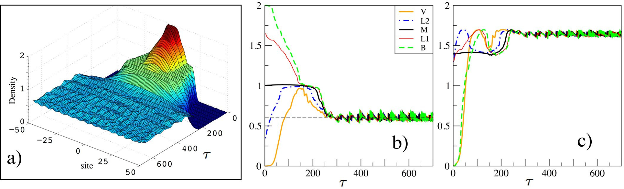
Panel a) of Fig. 2 illustrates the time-and-space resolved density profile resulting from a very slow ( i.e., a ”numerically adiabatic”) switching-off of the trap. For such a slow perturbation, and before the particles reach the boundaries, the results can be interpreted in terms of trapped-equilibrium-systems considerations [7, 11] (see below). However, in the following we find useful to adopt a time-dependent perspective, which remains appropriate also for faster switching-off of the trap.
At time the initial density profile is that of Fig. 1. As expected for adiabatic switching, for very long times the density evolves towards the ground state of the unconfined system, which in our case corresponds to a uniform distribution of fermions over sites on a ring.
Panel b) shows explicitly the time evolution of the five representative sites. All sites ultimately attain this density, but in very different ways. The metallic regions L1 and L2 start evolving towards as soon as the trap is reduced. Similarly, the vacuum region (V) gets filled up almost immediately. However, at intermediate times, roughly between and , the vacuum receives more fermions than would correspond to the uniform final state.
The densities in the Mott regions (M), on the other hand, maintain their value until , i.e. a persistency of the Mott phase is observed: This is consistent with previous work [15, 16, 29]. Furthermore, when the density at the originally metallic sites reaches 1 from above (L1) or below (L2), it, too, develops the characteristic Mott behavior and persists for an extended period of time. The corresponding transient flat regions are clearly visible in the curves labelled L1 and L2 in panel b). Differently from the Mott phase, the band insulator starts evolving towards the uniform state as soon as the trap begins to be reduced. This points at a basic difference between band and Mott insulators: The Mott insulator self-stabilizes due to particle-particle interactions, while the band insulator requires an external potential to be stable. Panel c) shows the time evolution of the EE. In contrast with the density results, the entanglement curves for vacuum and band insulating regions display very similar behavior. From an equilibrium-regime perspective, the above results can be rationalized in terms of energetics arguments [7, 11]: in strong traps band and Mott insulators coexist with compressible domains. As the trap curvature is reduced, the band insulator becomes energetically unfavorable, while the Mott insulator is sustained due to the rigidity arising from the discontinuity in . Also, the vacuum and band insulating regions, which have very different density profiles, display very similar EE behaviour; this is because the EE is related to the degrees of freedom that are available for storing or recovering information, and this number is zero if a site is completely filled or empty.
Results for moderate switching-off of the trap are in Figure 3. The overall features of the adiabatic curves are preserved, but compressed in a shorter timescale. For example, for long times the entanglement entropy evolves towards that of the uniform system, but again with significant delay for the Mott insulator, which exhibits resistance against melting until about . We note, however, also some differences from Fig. 2, e.g. for long times the density (and the EE) oscillates around the uniform state. Unlike the total particle number, the total EE is not conserved, and reaches, not necessarily in a monotonic way, a maximum at long times. In equilibrium, extrema of the EE are known [20, 21, 22, 23] to be markers of quantum phase transitions. In Figs. 2,3, the transitions from a Luttinger liquid to a Mott insulator and from Mott to Luttinger correspond to extrema in the EE. In principle, such correspondence might be spoiled away from equilibrium. Our simulations show, however, that this is not necessarily the case.
Finally, Fig. 4 refers to instantaneous switching. Both density and entanglement entropy show strong oscillations on a short time scale. Most likely, such oscillations are an artifact of our ALDA ; indirect evidence for this also comes from tDMRG studies of sudden quenches of the confining potential, which show a smooth expansion of the density profiles [16, 29, 30]. The main aim of Fig. 4 is to show an instance where the ALDA (but not lattice TDDFT [34]) scheme becomes inadequate. By contrast, the lattice TDDFT-ALDA [34] should be useful to follow the long-time evolution for slow and moderately fast switching off, i.e. situations which currently are not easily accessible within tDMRG calculations.

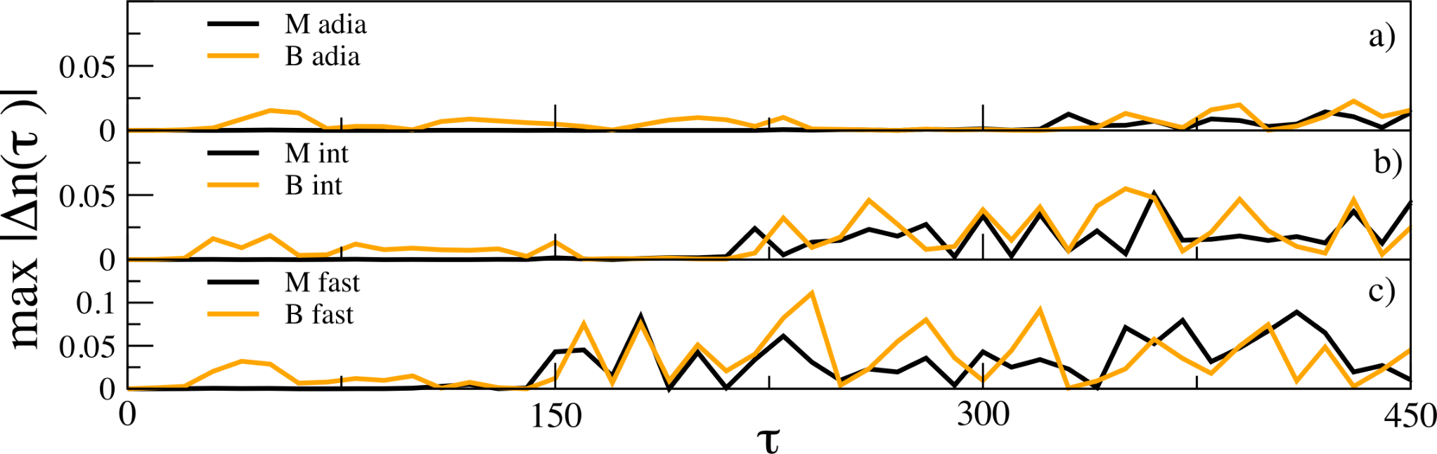
It is useful, at this stage, to quantify of the degree of adiabaticity in our results. To this end, we show in Fig. 5 three switching-off speeds. At each time , we considered the maximum difference (among all sites) between the time evolved densities and those obtained by the instantaneous ground state of the Hamiltonian. One sees that the TD results of Fig. 2 are quite close to the instantaneous ground states ones. On the other hand, for faster perturbations, the differences are more noticeable, a sign of significant departure from adiabaticity.
We stress that these findings are not related to a particular choice of the system parameters. We observed (not shown) the same behaviour in simulations with different amplitude modulations, numbers of fermions and lattice sites, different values for the on-site interaction, etc. [39].
5 Thermalization, ground state, and TDDFT
Our time-evolution results permit to address two other interesting issues within TDDFT, namely the system’s thermalization (i.e. the achievement of local equilibrium through interactions among the particles) and if it possible or not for the system to reach the ground state, once the trap is removed.
Generally, achieving thermalization or attaining the ground state are distinct processes: In general, after a parameter quench, in a finite system a ground state is not reached without exchange of energy; by contrast, thermalization is possible also when the system remains isolated after the quench. Thus, even for our zero-temperature calculations, thermalization remains a meaningful concept. As an indicator of local equilibrium in the long-time limit we can use the average value of a suitable one-body operator. In the case of TDDFT, the one-particle density is a natural choice.
For finite isolated systems, exact diagonalization studies have shown that, under quite general conditions, thermalization occurs [40]. On the other hand, experimental results for 1D interacting bosons [41] and several theoretical studies [42, 43, 44, 45] indicate that, in some cases, the quasi-stationary states after an interaction quench can be non-thermal. Overall, it is fair to say that, at present, the issue of thermalization in the presence of a global quench is not completely settled yet.
In our present context, these generic remarks suggest the following specific questions from a TDDFT perspective: i) How does thermalization occur in our system, when the confining potential is removed? ii) What is the relation between the state reached by our system in the long time regime and the ground state of the final Hamiltonian? To briefly address these points, let us first consider for definiteness the exact many-body dynamics of our system, Eq.(2), for two kinds of perturbations: i) sudden and ii) adiabatic. In the initial ground state with energy , the parabolic potential contributes a positive energy . After a sudden removal of the parabolic trap (as in Fig.4), the system has a new, time independent Hamiltonian , but the same initial state and the (initial) average energy is conserved at all times. Since, in general, , our system may thermalize, but cannot reach the ground state. On the other hand, if no symmetry restriction apply, when energy is removed from the system continuously and infinitely slowly (adiabatic switch-off of , as in Fig. 2), the ground state can be reached. For ”intermediate-speed” perturbations, as in Fig.3, in general thermalization may occur, even if the system does not reach the ground state.
In an exact TDDFT description, the exact TD density is accessed. Hence, the considerations above about thermalization and/or reaching the ground state still hold. However, the adiabatic BA-LDA used here is a local approximation in space and time, and thus dissipative effects are neglected. Consequently, the possibility that the system’s thermalization is described incorrectly cannot be ruled out. For example, within the simulation interval considered, the results of Fig. 4 show no indication that a uniform density (indicative of thermalization within TDDFT) is going to be established. On the other hand, for a very slow (adiabatic in a numerical sense) removal of the trap, such as in Fig.2, our treatment is expected to be quite accurate in describing the way the system approaches the ground state.
6 Conclusions
In summary, our simulations show that (i) the time evolution of the expanding cloud displays a wide variety of non-equilibrium phenomena (overshooting, transients, self-induced stability, etc), all of which should be experimentally accessible with todays technology. In particular, optical experiments can be used to investigate the time evolution of the Mott insulator – a state of matter that in ordinary condensed-matter situations can only be studied in static situations; (ii) a connection between the entanglement entropy and phase changes is observed also in non-equilibrium situations, thus suggesting the possibility of investigations and applications of quantum information concepts in dynamical settings; and (iii) if accurate enough potentials are used, TDDFT is a useful tool for characterizing and analyzing the long-time behavior of the expanding cloud, and to describe phenomena such as the approach to the ground state or the thermalization of initial states that are far from equilibrium.
Acknowledgements.
CV is supported by ETSF (INFRA-2007-211956). KC is supported by FAPESP and CNPq.References
- [2] I. Bloch, J. Dalibard and W. Zwerger, Rev. Mod. Phys. 80, 885 (2008). S. Giorgini, L. P. Pitaevskii and S. Stringari, Rev. Mod. Phys. 80, (2008) 1215.
- [3] R. Jördens, N. Strohmaier, K. Günter, H. Moritz and T. Esslinger, Nature 455, (2008) 204.
- [4] M. Greiner and S. Fölling, Nature 453, (2008) 736.
- [5] For a recent review, see for example T. Lahaye, C. Menotti, L. Santos, M Lewenstein and T. Pfau, Rep. Prog. Phys 72, (2009) 126401.
- [6] A. Koga, T. Higashiyama, K. Inaba, S. Suga, and N. Kawakami, J. Phys. Soc. Jpn. 77, (2008) 073602.
- [7] M. Rigol, A. Muramatsu, G.G. Batrouni, and R.T. Scalettar, Phys. Rev. Lett. 91, (2003) 130403. M. Rigol and A. Muramatsu, Phys. Rev. A 69, (2004) 053612.
- [8] X.-J. Liu, P.D. Drummond, and H. Hu, Phys. Rev. Lett. 94, (2005) 136406.
- [9] G. Xianlong, M. Polini, M. P. Tosi, V. L. Campo, Jr., K. Capelle and M. Rigol, Phys. Rev. B 73, (2006) 165120.
- [10] U. Schneider, L. Hackermüller, S. Will, Th. Best, I. Bloch, T. A. Costi, R. W. Helmes, D. Rasch and A. Rosch, Science 322, (2008) 1520.
- [11] V. L. Campo, Jr. and K. Capelle, Phys. Rev. A 72, (2005) 061602(R).
- [12] W. Li, G. Xianlong, C. Kollath and M. Polini, Phys. Rev. B 78, (2008) 195109.
- [13] C. Kollath, U. Schollwöck and W. Zwerger, Phys. Rev. Lett. 95, (2005) 176401.
- [14] C. H. Schunck, M. W. Zwierlein, A. Schirotzek, and W. Ketterle, Phys. Rev. Lett. 98, (2007) 050404.
- [15] A. Rosch, D. Rasch, B. Binz, and M. Vojta, Phys. Rev. Lett. 101, (2008) 265301.
- [16] F. Heidrich-Meisner, M. Rigol, A. Muramatsu, A. E. Feiguin and E. Dagotto, Phys. Rev. A 78, (2008) 013620.
- [17] F. Massel, M. J. Leskinen and P. Törmä, Phys. Rev. Lett. 103, (2009) 066404.
- [18] E. Haller, M. Gustavsson, M. J. Markiewisz, J. G. Danzl, R. Hart, G. Pupillo, H.-C. Nägerl, Science 325, (2009) 1224.
- [19] E. A. L. Henn, J. A. Seman, G. Roati, K. M. F. Magalhaes and V. S. Bagnato, Phys. Rev. Lett. 103, (2009) 045301.
- [20] A. Osterloh, L. Amico, G. Falci and R. Fazio, Nature 416, (2002) 608. T. J. Osborne and M. A. Nielsen, Phys. Rev. A 66, (2002) 032110.
- [21] L.-A. Wu, M. S. Sarandy and D. A. Lidar, Phys. Rev. Lett. 93, (2004) 250404. L.-A. Wu, M. S. Sarandy, D. A. Lidar and L. J. Sham, Phys. Rev. A 74, (2006) 052335.
- [22] D. Larsson and H. Johannesson, Phys. Rev. Lett. 95, (2005) 196406, ibid. 96, (2006) 169906(E).
- [23] V. V. Franca and K. Capelle, Phys. Rev. A 74, (2006) 042325.
- [24] A. M. Läuchli and C. Kollath, J. Stat. Mech. 2008, (2008) P05018 .
- [25] G. Sadiek, Z. Huang, O. Aldossary and S. Kais, Mol. Phys. 106, (2008) 1777.
- [26] L. Qiu, A. M. Wang and X. Q. Su, Opt. Comm. 281, (2008) 4155.
- [27] M. Fagotti and P. Calabrese, Phys. Rev. A 78, (2008) 010306(R).
- [28] J. Fitzsimons and J. Twamley, Phys. Rev. A 72, (2005) 050301(R).
- [29] F. Heidrich-Meisner, S. R. Manmana, M. Rigol, A. Muramatsu, A. E. Feiguin, E. Dagotto, Phys. Rev. A 80, (2009) 041603.
- [30] K. Rodriguez, S. R. Manmana, M. Rigol, R. M. Noack, A. Muramatsu, New. J. Phys 8, (2006) 169.
- [31] N. A. Lima, M. F. Silva, L. N. Oliveira and K. Capelle, Phys. Rev. Lett. 90, (2003) 146402.
- [32] K. Schönhammer, O. Gunnarsson, and R. M. Noack, Phys. Rev. B 52, (1995) 2504.
- [33] E. Runge and E. K. U. Gross, Phys. Rev. Lett. 52, (1984) 997.
- [34] C. Verdozzi, Phys. Rev. Lett. 101, (2008) 166401.
- [35] N. A. Lima, L. N. Oliveira and K. Capelle, Europhys. Lett. 60, (2002) 601.
- [36] D. Vieira, K. Capelle and C. A. Ullrich, Phys. Chem. Chem. Phys. 11, (2009) 4647.
- [37] S.-J. Gu, S.-S. Deng, Y.-Q. Li and H.-Q. Lin, Phys. Rev. Lett. 93, (2004) 086402.
- [38] V. V. Franca and K. Capelle, Phys. Rev. Lett. 100, (2008) 070403.
- [39] The expansion of a 2D cloud of lattice fermions has been recently examined experimentally and theoretically by U. Schneider, L. Hackermüller, J. P. Ronzheimer, S. Will, S. Braun, T. Best, I. Bloch, E. Demler, S. Mandt, D. Rasch, A. Rosch, arXiv:1005.3545v1.
- [40] M. Rigol, V. Dunjko and M. Olshanii, Nature 452, (2006) 854.
- [41] T. Kinoshita, T. Wenger, and D. S. Weiss, Nature (London) 440, (2006) 900.
- [42] M. A. Cazalilla, Phys. Rev. Lett. 97, (2006) 156403.
- [43] S. R. Manmana, S. Wessel, R. N. Noack, and A. Muramatsu, Phys. Rev. Lett. 98, (2007) 210405.
- [44] G. Biroli, C. Kollath, A. Laeuchli, arXiv:0907.3731
- [45] M. Kronenwett and T. Gasenzer, arXiv:1006.3330v1