Bound States of the Heavy Flavor Vector Mesons and and
Abstract
The and systems are studied dynamically in the one boson exchange model, where , , , and exchanges are taken into account. Ten allowed states with low spin parity are considered. We suggest that the , , and molecules should exist, and the bound states with the same quantum numbers very likely exist as well. However, the CP exotic (, ) and states may not be bound by the one boson exchange potential. We find that the configuration is more deeply bound than the configuration, hence may not be a molecule. Although is close to the threshold, the interpretation of as a molecule is not favored by its huge width. and states can be produced copiously in annihilation, detailed scanning of the annihilation data near the and threshold is an important check to our predictions.
pacs
12.39.Pn, 12.39.Jh, 12.40.Yx, 13.75.LbI Introduction
In the past years, the observations of a number of charmonium-like ”” mesons at factories have stimulated the interest in the spectroscopy of the charmonium states again. There is growing evidence that at least some of these new states are non-conventional states, such as deuteron like hadronic molecules, tetraquark states or hybrid have been suggested review. Among these new mesons, some are very close to the threshold of two charmed mesons, such as Choi:2003ue and Choi:2007wga; Aubert:2008nk. This distinctive character inspires the molecular interpretation for these mesons. In particular, some new enhancements near the threshold have been observed recently.
The Belle collaboration reported a broad peak near 4008 MeV in addition to the well-known state by studying the initial state radiation process Yuan:2007sj, its mass and width are fitted to be MeV and MeV respectively. We notice its width is huge. This peak was suggested to be related to the threshold and could be a molecule in Ref. Liu:2007ez. The spectrum was studied further by the Babar collaboration. However, there was no evidence for this broad enhancement, and the an upper limit at C.L. was obtained Aubert:2008ic. is far from being established so far, more experimental efforts are obviously needed.
Of special importance is the observation of the state carrying non-zero electric charge with hidden charm quarks. Since the observation of Choi:2007wga; Aubert:2008nk, the Belle collaboration reported two resonance-like structures and in the mass distribution in the exclusive process Mizuk:2008me. Their masses and widths are determined to be MeV, MeV, MeV and MeV respectively. Since is an isovector with negative G-parity, and is a isospin singlet with positive G-parity, the quantum numbers of both Z(4051) and Z(4250) are . In Ref.Liu:2008tn, was suggested to be possibly a molecule due to its closeness to the threshold. However, the QCD sum rule results indicated that the state is probably a virtual state, which is not related with the resonance-like structure Lee:2008gn. In addition, we demonstrated that as a or molecule is disfavored in Ref. Ding:2008gr.
Since the repulsive kinetic energy is greatly reduced by the heavy quark mass, the interaction between light quarks is strong enough so that the molecular states consisting of heavy flavor mesons very likely exist. In fact, the hadronic molecules consisting of two charm mesons were suggested long ago Voloshin:1976ap. De Rujula, Georgi and Glashow proposed that the molecular states involving hidden pair do exist, and have a rich spectrum De Rujula:1976qd. Possible new resonance near the threshold was suggested by Voloshin Voloshin:2006wf; Dubynskiy:2006sg. Different from other possible exotic structures, there are uncontroversial evidences for hadronic molecule such as the deuteron, which is unambiguously a proton-neutron bound state. The deuteron has been studied in great details over the years Ericson:1985hf; Ericson:1982ei. From these studies, we learn that the pion exchange determines most of the binding energy and the long range part of the deuteron wavefunction, and the S-D wave mixing effect plays a critical role in providing the binding. Guided by the binding of deuteron, Tornqvist performed a systematic study of possible deuteronlike two mesons bound states with long distance one pion exchange Tornqvist:1991ks; Tornqvist:1993ng. At short distance, the interaction should be induced by the interactions among the quarks. However, a detailed and reliable modelling of the short range interaction is not a easy matter, and various phenomenological models have been proposed Barnes:1991em; Swanson:1992ec, although one pion exchange is expected to be dominant for the hadronic molecule. Inspired by the nucleon-nucleon interactions, we further extended the one pion exchange model to include the short distance contributions from the heavier bosons , , and exchanges in Ref. Ding:2009vj. We have also taken into account the contribution of the ” function” term, which leads to a function term in the effective potential in configuration space when no regularization is used. This one boson exchange model gives a very good description of the weakly bound hadronic molecule. It has been successfully applied to exploring the possible heavy flavor pseudoscalar-vector molecular states Ding:2009vj, the system and the molecular interpretation of Ding:2009vd. Motivated by the controversial states and , we shall examine for which quantum numbers the boson exchange potential is attractive and strong enough so that bound states are expected, ten allowed states with low spin parity are considered. Moreover, the system would be discussed as well.
The paper is organized as follows. In section II, the formalism of one boson exchange model is summarized. In section III, we apply the one boson exchange model to the system, the quantum numbers of the bound states which might exist, are suggested. The system is discussed along the same line in section IV. Finally we present our conclusions and some discussions in section V.
II The formalism of the one boson exchange model
In the one boson exchange model, the effective potential between two hadrons is obtained by summing the interactions between light quarks or antiquarks via one boson exchange. To leading order in the boson fields and their derivative, the effective interactions between the constituent quark and the exchanged boson are as follows Nagels:1975fb; Nagels:1977ze; Machleidt:1987hj; Ding:2009vj
| (1) |
Here is the constituent quark mass, is the constituent quark Dirac spinor field, , and are isospin-singlet pseudoscalar, scalar and vector boson fields respectively. In this work we take MeV, since we concentrate on the constituent up and down quarks here. If the isovector bosons are involved, the couplings enter in the form , and respectively, where is the well-known Pauli matrices. Following standard procedure, we can straightforwardly obtain the one boson exchange potential between two quarks.
- 1.
Pseudoscalar boson exchange
(2) where is the tensor operator. We have defined to approximately account for the recoil effect due to the small mass splitting within the heavy flavor vector meson isospin multiplet Tornqvist:1991ks; Tornqvist:1993ng; Thomas:2008ja, where is the exchanged pseudoscalar mass, and are the masses of the heavy flavor vector mesons involved. For the system, the mass splitting can be negligible so that is satisfied.
- 2.
Scalar boson exchange
(3) where , with being the exchanged scalar meson mass, and is the angular momentum operator.
- 3.
The dimensionless functions , , and introduced in Eq.(2)-Eq.(4) are defined as follows
| (5) |
with . In deriving the above effective potentials, we have introduced form factor at each interaction vertex to regularize the effective potential at short distance, and the form factor in momentum space is taken as
| (6) |
where is the so-called regularization parameter, and are the mass and the four momentum of the exchanged boson respectively. This form factor suppresses the contribution of high momentum, i.e. small distance. The presence of such a form factor is dictated by the extended structure of the hadrons. The parameter , which governs the range of suppression, can be directly related to the hadron size which is approximately proportional to . However, since the question of hadron size is still very much open, the value of is poorly known phenomenologically, and it is dependent on the models and applications. In the nucleon-nucleon interactions, the in the range of 0.8-1.5 GeV has been used to fit the data. For the present application to the heavy flavor vector mesons system, which have a smaller size than the nucleon, we would expect a larger regularization parameter . We have demonstrated that the binding energy and static properties of the deuteron are produced very well in the one boson exchange model, if is chosen to be about 808 MeV Ding:2009vj. In the case that all coupling constants except are reduced by half, should be approximately MeV. The extended structure of hadrons also has the following obvious consequence: because the mass of the exchanged meson determines the range of the corresponding contribution to the interactions, one should restrict oneself to meson exchange with the exchanged meson mass below a certain value, typically on the order of the regularization parameter . Since , , , and exchanges are considered in the present work, the value of should be larger than the meson mass.
In the present one boson exchange model, the input parameters include the masses of the exchanged bosons and heavy flavor vector mesons, and the effective coupling constants between the constituent quarks and the exchanged bosons. The meson masses are taken from the compilation of the Particle Data Group pdg: MeV, MeV, MeV, MeV, MeV, MeV, MeV, MeV and MeV. The constituent quark-meson coupling constants can be estimated from the phenomenologically known , , , and coupling constants via the well-known Goldberger-Treiman relation Ding:2009vj; Riska:2000gd.
| (7) |
Among the above effective boson-nucleon coupling constants, only has been determined accurately from the pion-nucleon and nucleon-nucleon scatterings. As in our previous work Ding:2009vj; Ding:2009vd, the effective coupling constants are taken from the famous Bonn model Machleidt:1987hj. The uncertainty of the coupling constants will be taken into account later, all the coupling constants except are reduced by half for demonstration, and the corresponding numerical results are presented as well.
For the system consisting of two vector mesons, the spatial parity is determined by and the parity is , where is the relative angular momentum between two vector mesons, and is the total spin of the system. We cutoff the total angular momentum of the system to , the allowed states with low spin parity are listed in Table 1. In the following, we shall study for which quantum numbers the one boson exchange potential is so attractive that bound states may exist.
| Channels | |
|---|---|
| , | |
| , | |
| , , | |
| , , , | |
| , | |
| , |
III The possible molecular states of the system

There is a sign difference between the quark-quark interactions and quark-antiquark interactions, the magnitudes are the same, where is the -parity of the exchanged meson. Consequently both and exchanges give opposite sign between quark-quark interactions and quark-antiquark interactions. In the present case, the effective potential is induced by one boson exchange between a pair of light quark and antiquark, and the diagram contributing to interactions is shown in Fig. 1. The effective potential is explicitly expressed as
| (8) | |||||
where (, , , and ) denotes the effective potential induced by the meson exchange between two quarks. The subscripts and are the indexes of light quark and antiquark. The spin operator(isospin operator) or ( or ) only acts on the light quark and antiquark. The parameters , and could take two different sets of values due to the small mass splitting within the and isospin multiplets. For and , we should choose , and . Whereas for the and processes, we should take , and . The eight potential functions , etc are given by
| (9) |
Since the threshold of is about 6.6 MeV higher than the threshold, the isospin symmetry is expected to be violated drastically for the molecular states whose binding energy is of order a few MeV Ding:2009vj. Isospin violation mainly comes from three aspects: the first is the different kinetic energies for and , the second is the different effective potentials from exchange and exchange, and the third is because of the different thresholds of and . In the following, we will perform the same analysis as that for the deuteron and the possible heavy flavor molecules in Ref. Ding:2009vj; Ding:2009vd. One can then determine for which quantum numbers the one boson exchange potential is attractive and strong enough so that the bound states are expected. Firstly we consider the states as an demonstration, the system can be in S wave or D wave similar to the deuteron. Taking into account the isospin violation effect, one has four coupled channels. For convenience, we choose the basis to be , , and , then the wavefunction of the system is written as
| (10) |
where , , and are the spatial wavefunctions. The matrix elements of the light quark relevant operators , and etc in Eq.(8) can be calculated straightforwardly with the help of angular momentum algebra, and the results are given analytically in the Appendix of Ref.Ding:2009vj. Consequently the one boson exchange potential for the state can be written in the matrix form as
For the up-left and down-right matrix elements, we should choose , and . While for the off-diagonal matrix elements, we should take , and . Taking into account the D wave centrifugal barrier and solving the coupled channel Schrdinger equation numerically, the numerical results are listed in the Table 2. It is obvious that the binding energy and the static properties are rather sensitive to the regularization parameter and the effective coupling constants, this is common to the one boson exchange model Ding:2009vj; Ding:2009vd; Thomas:2008ja. We also find that the binding energy increases with , this is because increasing increases the strength of the potential at short distance. For MeV, a bound state with mass about 4013.80 MeV appears. We can see that the isospin symmetry is strongly broken especially for the states near the threshold. Fig. 2 displays the wavefunction of the bound state with mass 4004.40 MeV and MeV. One notice that the component dominates over the component for both the S wave and D wave configurations, as could be expected. Because the wavefunctions and have the same sign, the same is true for and . Therefore the component is predominant for this state, it would be an isospin singlet in the isospin symmetry limit. The dominance of the configuration is observed for all the states listed in Table 2. From the numerical results, we can see that the D wave probability increases with the regularization parameter , the importance of the tensor force is obvious. The uncertainties induced by the effective coupling constants are considered as well. All the coupling constants except are reduced by half, and the corresponding numerical results are presented in Table 2. The same pattern of the static properties dependence on is found. Bound state solution appears if the regularization parameter is about MeV, the value of is still in the reasonable range. Since the molecular state is widely extended, the decay into light mesons via annihilation is generally suppressed by the form factor. The leading source of decay is dissociation, to a good approximation the dissociation will proceed via the almost free space decay of the constituent mesons. Consequently the molecule mainly decays into , and , and the mode is strongly suppressed or even forbidden by the phase space.

The one boson exchange potentials for the nine remaining states are listed in Appendix A. Following exactly the same method, the binding energy and the static properties can be predicted, and partial results are shown in Appendix B for illustration. The binding energy and the static properties are found to be rather sensitive the regularization parameter . The spatial wavefunctions for the and components have the same sign, consequently the component is dominant for all these states, and they are isospin singlets in the isospin symmetry limit. The same conclusion has been reached in the one pion exchange model Tornqvist:1993ng, where the strength of the effective potential for the state is about one third of that for . We shall discuss these states one by one in the following.
For the axial vector state, there are four channels (), (), () and (). The energy of the system is substantially lowered due to the S-D wave mixing effect. The coupling between the S wave and D wave has the same strength as the case, which is clearly seen from Eq.(III) and Eq.(A). It is obvious that the predictions for the binding energy and the static properties have similar pattern with the ones for the state, and the binding of the state is less stronger than the one for the same value. For as large as 980 MeV, we can find a bound state with mass about 4012.43 MeV. If all coupling constants except are reduced by half, bound state begins to appear for MeV. We note that the unnatural spin parity forbids its decay into , while the decay mode is allowed.
The pseudoscalar state involve two channels () and (). If the small isospin violation effect is neglected, the two coupled channel problem is reduced to a familiar one channel problem. Although there is repulsive P wave centrifugal barrier, the one boson exchange potential is so strong that the P wave centrifugal barrier can be partly compensated, therefore bound state solutions can be found for reasonable values of , as can be seen from Table 3. For MeV, we find that the binding energy with respect to the threshold is in the range of 2.6 to 137.2 MeV. The binding energy is more sensitive to than the and four coupled channels cases. The probabilities for the () and () components are close to each other, as could be expected. The small difference is induced by the mass splitting within the and isospin multiplet.
The results for the state are similar to the case. Because the D wave centrifugal barrier is higher than the P wave centrifugal barrier, the total effective potential for the state is less attractive than the state. If the coupling constants except are reduced by half, bound state solutions can be found only for larger than 1290 MeV. Since the numerical results indicate that larger value of is required to bind the state, the state is harder to be bound than the previous states considered.
For the CP exotic and states, the system is in P wave and D wave respectively. Considering isospin violation effect, two channels are involved for both states. As has been shown in Eq.(A) and Eq.(A), the one boson exchange potentials for these two states are exactly the same, and they are less attractive than the potentials for the and states. For the state, bound state solution appears only for as large as 1300 MeV, and we can find bound state only if the regularization parameter is larger than 1640 MeV. If we reduce all the coupling constants except by half, larger than 3010 MeV and 5110 MeV respectively for the and states is required to find bound state solutions. Because the value of is so large that it is far beyond the range of 0.8 to 1.5 GeV favored by the nucleon-nucleon interactions, we tend to conclude that the CP exotic and states can not be bound by the one boson exchange potential. This conclusion is consistent with the fact that no such CP exotic states have been observed so far.
We then come to the very interesting state, there are six configurations (), (), (), (), () and ( ). Due to the substantially strong attraction of the effective potential, bound state solutions can be found for reasonable value of in spite of the P wave centrifugal barrier. The wavefunction of the bound state with mass about 4006.82 MeV and MeV is displayed in Fig. 3. From the numerical results in Table 4, we see that the isospin symmetry is violated, especially for the states near the threshold. The () and () are the dominant components, the components are strongly suppressed by the large F wave centrifugal barrier. For the same value of the regularization parameter , we notice that the binding energy of state is the largest among the ten allowed states. Hence we suggest that the molecular state should exist, this conclusion is consistent with the results obtained from the general quantum mechanical properties of unitarity and analyticity Voloshin:2006wf; Dubynskiy:2006sg. The state is remarkable, it can be directly produced via the annihilation or with the help of the initial state radiation (ISR) technique at factory. The existence of such a state can be either confirmed or rejected if more detailed annihilation data near the threshold become available. We strongly urge the Babar and Belle collaboration to search for this state. The molecule mainly decays into and via the dissociation of and , the decays into and are allowed as well. The width of the molecule should be of the same order as the width. Therefore it would be be a narrow state, and its width is expected to be of the order about 10 MeV. For the state reported by the Belle collaboration, although it is close to the threshold, its width is huge, which is MeV. Consequently it seems unreasonable to interpret as the molecule.

For the state, eight channels (), (), (), (), (), (), ( ) and () are involved. The effective potential in matrix form is given in Eq.(A), which is more complex than the previous cases considered. It is obvious that both the tensor interaction and the spin-orbit interaction vanish in the configuration. However, bound state solution can be found for reasonable value of ( should be larger than 860 MeV and 970 MeV respectively for the two sets of coupling constant values). The reason is that the mixing of with , and under the tensor force increases the binding of the system considerably through higher order iterative processes. We show the wavefunction of the molecular state with mass 4010.82 MeV and MeV in Fig. 4. Isospin violation is obvious, and the component is dominant. From the numerical results presented in Table 5, we can see that () and () are the dominant components, the probability is larger than the probability, and the component is suppressed. It is remarkable that the dependence of the state mass on is the least sensitive among the ten allowed states. Comparing the numerical results presented in Table 2 and Table 5, it can be seen that the binding of this state is comparable to the state, accordingly the molecule very likely exist.

Finally two states with and respectively remain. For both states, one has four coupled channels, P wave and F wave configurations are involved. Because of the P wave and F wave centrifugal barrier, bound state begins to appear for as large as 1150 MeV and 1090 MeV respectively. If all the coupling constants except are reduced by half, the value of should be larger than 1630 MeV and 1480 MeV respectively in order to find bound state solutions. We tend to conclude that the one boson exchange potential may not support the and states.
In short summary, ten allowed states with low spin parity has been studied. We find that the isospin symmetry is violated, especially for the states near the threshold. The configuration is dominant for all the lowest bound states, hence they would be isospin singlets in the isospin symmetry limit. Since is an isospin vector, as a molecule is not favored. This conclusion is consistent with the prediction from the QCD sum rule Lee:2008gn. We suggest that the , , and molecules should very likely exist, whereas the CP exotic and states, and states should not be bound by the one boson exchange potential. Although is close to the threshold, its width is so large that it is not reasonable to identify as a molecule. The molecular state can be produced copiously in annihilation or via the initial state radiation at factory, detailed scan of the annihilation data near the threshold is crucial to confirming this prediction.
IV The molecular states of the system
The mass difference between and is so small that it can be negligible pdg. If we take into account the mass splitting within the exchanged pion isospin multiplet, we should solve similar coupled channel problems as the case. The repulsive kinetic energy is greatly reduced due to the larger mass of meson, therefore the system should be more deeply bound than the system. Numerically solving the corresponding Schrdinger equation, we notice that the molecular states bound for reasonable value have definite isospin, and the configuration is obviously much easier to be bound than the configuration. We also find that the binding energy dependence on becomes less sensitive, if we reduce all the coupling constants except by half. In the case that the mass difference between and is neglected, the state is of definite isospin, and the dimensions of the coupled channel equations would be reduced by half. We have seriously calculated the binding energy and the static properties for both the and states. However, the numerical results are too lengthy to be listed in the manuscript. We find that introducing the pion mass splitting will modify the binding energy by at most 0.5 MeV.
For the and system, both the and bound states can be found for the same value of the regularization parameter , whereas the two states behave in different way. The state is generally more deeply bound than the state. For the isospin singlet, the D wave components increase drastically with . Whereas for the isospin vector, the S wave components are dominant, and they increase slightly with . Because mainly decays into pdg, is the leading decay mode of the molecule via the and dissociation. For the eight remaining states, we also find that the configuration is more tightly bound than the configuration, hence it seems to be a universal result that the hadronic molecule prefers to a isospin singlet.
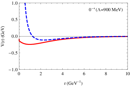
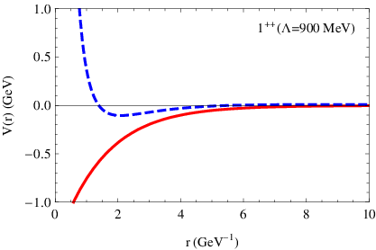
Since the mass splitting within the pion isospin multiplet only introduces minor modifications. The numerical results can be understood easily in the exact isospin symmetry limit. If the pion mass splitting is neglected, the , , and states only involve one channel. Both the one boson exchange potential and the total potential including the centrifugal barrier for the four states are displayed in Fig. 5. From Fig. 5a, we can see that the P wave centrifugal barrier is partly compensated by the one boson exchange potential, and there remains a weak attractive interaction in the intermediate range. Therefore bound state can be found for reasonable values of . For MeV, we find the binding energy is in the range of 2.93 to 134.71 MeV. Because the D wave centrifugal barrier is higher than the P wave centrifugal barrier, the total potential of the state is less attractive than the one for the same values of parameters, this point can be seen clearly by comparing Fig. 5b with Fig. 5a. Accordingly our numerical results really indicate that the state is harder to be bound than the state. For MeV, bound state can not be found, it is because the potential including the P wave centrifugal barrier is repulsive in this case. When is increased to about 1120 MeV, the total potential shown in Fig. 5d becomes attractive in the intermediate region, the system is marginally bound. The one boson exchange potentials for the CP exotic and states are exactly the same. However, the system is more loosely bound than the system because of the D wave centrifugal barrier. Fig. 5e and Fig. 5f clearly show that the total potential of the state is still repulsive for both MeV and 1120 MeV. bound state begins to appear for as large as 1260 MeV.
 |
 |
 |
| (a) | (b) | (c) |
 |
 |
 |
| (d) | (e) | (f) |
The dominance of the configuration over can be clearly understood as well for the , , and states in the isospin symmetry limit. In this case, the one boson exchange potential is the summation of the isospin independent part and multiplying the isospin relevant part, where the parameter is equal to -3 and 1 respectively for and 1. Concretely for the state, the isospin independent potential is , and the isospin relevant part is . We plot both the isospin irrelevant and relevant potentials for these states in Fig. 6, it is obvious that the isospin irrelevant potential is usually attractive. For the and states with MeV, the isospin relevant potential is positive, hence it is easily understood why the configuration is more attractive than . For the state with MeV, the isospin relevant part is negative, thus the potential for the state is deeper than the one for . However, the corresponding potential still can not support a isovector state, such state can be bound only when is increased to about MeV. For as large as 1120 MeV, the isospin relevant potential becomes positive, accordingly the configuration is more tightly bound than . In this case, a marginally bound isospin singlet appears with mass about 10635.39 MeV. If we reduce all the coupling constants except by half, the and states can be bound only if is larger than 1700 MeV and MeV respectively. Therefore the one boson exchange potential may not support the CP exotic and molecules.
 |
 |
 |
 |
| (a) | (b) | (c) | (d) |
Following the same methhod as the case and carefully examining the numerical results, we suggest that the , , and molecules should exist, and the bound state also very likely exists. Similar to the state, the molecule can be produced largely in annihilation at Babar or Belle. Detailed scanning of the annihilation data at the threshold is expected.
V Conclusions and discussions
Motivated by the charmonium-like state and , the possible molecular states have been studied dynamically in the one boson exchange model, where , , , and exchanges are taken into account. Ten allowed states with low spin parity have been considered. We find that the binding energy and static properties are sensitive to the regularization parameter and the effective coupling constants. The binding energy increases with , whereas the root of mean square radius decreases with , this is because increasing increases the strength of the potential at short distance. Larger coupling constants are favorable to the formation of molecular states. If all the coupling constants except are reduced by half, larger value of is required to find bound state solutions. Isospin violation is expected, especially for the states close to the threshold, and the component is dominant, The predominance of the configuration over can be clearly understood in the exact isospin symmetry limit, and the same conclusion is reached in the one pion exchange model. Hence the interpretation of as a molecule is not favored.
Since the regularization parameter is poorly known so far, we are not be able to precisely predict the binding energies for the possible molecular states bound by one boson exchange potential. Certainly, if the potential is strong enough one can be quite confident that such bound state must exist, but their exact binding energy always depends on the details of the regularization procedure. However, we can reliably predict which ones of the ten allowed states are much easier to be bound, and the prediction is rather stable even if the uncertainty of the coupling constants is considered, as is obvious from the numerical results in Appendix B. Further research on X(3872) would put severe constraint on the parameters on the one boson exchange model, especially on the regularization parameter , so that the predictions presented in the work could become more precise.
Our detailed numerical results indicate that the , , and bound states should very likely exist, whereas the CP exotic and states, and states may not be bound by the one boson exchange potential. The state can be directly produced in annihilation, detailed annihilation data near the threshold are important to confirm or refute the existence of such state. The molecule mainly decays into and via the dissociation of and , the mode is highly suppressed or forbidden by the phase space, and its width should be about tens of MeV. Although is close to the threshold, its width is huge so that it is unreasonable to identify as a molecule. The existence of and has not been confirmed so far, more experimental efforts are urgently needed.
The possible molecular states have been discussed along the same line. The system is more deeply bound than the system. We find that the molecular states of the system have definite isospin, and the isospin singlet is much easier to be bound than the isospin vector for the states considered, the reason is analyzed in the isospin symmetry limit. If the small isospin mass splitting between the neutral and charged pion mesons is neglected, the dimension of the coupled channel problem is reduced by half, the situation is simplified greatly. It is observed that including the pion mass splitting modifies the binding energy by at most 0.5 MeV. We suggest that the , , and molecules should exist, they would be narrow states, and they dominantly decay into .
Acknowledgements.
We are grateful to Prof. Mu-Lin Yan and Dao-Neng Gao for stimulating discussions. This work is supported by the China Postdoctoral Science Foundation (20070420735), K.C. Wong Education Foundation, and KJCX2-YW-N29 of the Chinese Academy.References
- (1) E. S. Swanson, Phys. Rept. 429, 243 (2006), arXiv:hep-ph/0601110; S. Godfrey and S. L. Olsen, Ann. Rev. Nucl. Part. Sci. 58, 51 (2008), arXiv:0801.3867 [hep-ph]. .
- (2) S. K. Choi et al. [Belle Collaboration], Phys. Rev. Lett. 91, 262001 (2003), arXiv:hep-ex/0309032.
- (3) S. K. Choi et al. [Belle Collaboration], Phys. Rev. Lett. 100, 142001 (2008), arXiv:0708.1790 [hep-ex].
- (4) B. Aubert et al. [BaBar Collaboration], arXiv:0811.0564 [hep-ex].
- (5) C. Z. Yuan et al. [Belle Collaboration], Phys. Rev. Lett. 99, 182004 (2007), arXiv:0707.2541 [hep-ex].
- (6) X. Liu, Eur. Phys. J. C 54, 471 (2008), arXiv:0708.4167 [hep-ph].
- (7) B. Aubert et al. [BaBar Collaboration], arXiv:0808.1543 [hep-ex].
- (8) R. Mizuk et al. [Belle Collaboration], Phys. Rev. D 78, 072004 (2008), arXiv:0806.4098 [hep-ex].
- (9) X. Liu, Z. G. Luo, Y. R. Liu and S. L. Zhu, arXiv:0808.0073 [hep-ph].
- (10) S. H. Lee, K. Morita and M. Nielsen, Nucl. Phys. A 815, 29 (2009), arXiv:0808.0690 [hep-ph].
- (11) G. J. Ding, Phys. Rev. D 79, 014001 (2009), arXiv:0809.4818 [hep-ph].
- (12) M. B. Voloshin and L. B. Okun, JETP Lett. 23, 333 (1976) [Pisma Zh. Eksp. Teor. Fiz. 23, 369 (1976)].
- (13) A. De Rujula, H. Georgi and S. L. Glashow, Phys. Rev. Lett. 38, 317 (1977).
- (14) M. B. Voloshin, In the Proceedings of 4th Flavor Physics and CP Violation Conference (FPCP 2006), Vancouver, British Columbia, Canada, 9-12 Apr 2006, pp 014, arXiv:hep-ph/0605063.
- (15) S. Dubynskiy and M. B. Voloshin, Mod. Phys. Lett. A 21, 2779 (2006), arXiv:hep-ph/0608179.
- (16) T. E. O. Ericson and M. Rosa-Clot, Ann. Rev. Nucl. Part. Sci. 35, 271 (1985).
- (17) T. E. O. Ericson and M. Rosa-Clot, Nucl. Phys. A 405, 497 (1983).
- (18) N. A. Tornqvist, Phys. Rev. Lett. 67, 556 (1991).
- (19) N. A. Tornqvist, Z. Phys. C 61, 525 (1994), arXiv:hep-ph/9310247.
- (20) T. Barnes and E. S. Swanson, Phys. Rev. D 46, 131 (1992).
- (21) E. S. Swanson, Annals Phys. 220, 73 (1992).
- (22) G. J. Ding, J. F. Liu and M. L. Yan, Phys. Rev. D 79, 054005 (2009), arXiv:0901.0426 [hep-ph].
- (23) G. J. Ding, arXiv:0904.1782 [hep-ph].
- (24) M. M. Nagels, T. A. Rijken and J. J. de Swart, Phys. Rev. D 12, 744 (1975).
- (25) M. M. Nagels, T. A. Rijken and J. J. de Swart, Phys. Rev. D 17, 768 (1978).
- (26) R. Machleidt, K. Holinde and C. Elster, Phys. Rept. 149 (1987) 1.
- (27) C. E. Thomas and F. E. Close, Phys. Rev. D 78, 034007 (2008), arXiv:0805.3653 [hep-ph].
- (28) C. Amsler et al. (Particle Data Group), Phys. Lett. B667, 1 (2008).
- (29) D. O. Riska and G. E. Brown, Nucl. Phys. A 679, 577 (2001), arXiv:nucl-th/0005049.
Appendix A The one boson exchange potential for the () states including the isospin mass splitting
In the above expressions, the parameters , and could take two different sets of values. For () and (), we should choose , and . Whereas for the processes () and (), we should take , () and () respectively.
Appendix B Numerical results for the states
| 930 | 4013.80 | 8.24 | 95.69:1.80:0.50:2.01 |
|---|---|---|---|
| 940 | 4011.72 | 2.39 | 70.69:11.01:7.43:10.88 |
| 950 | 4004.40 | 1.36 | 39.99:22.32:16.38:21.31 |
| 960 | 3990.26 | 1.03 | 25.21:29.74:16.55:28.50 |
| 970 | 3968.64 | 0.86 | 17.70:34.73:14.01:33.57 |
| 980 | 3938.98 | 0.76 | 13.19:38.20:11.41:37.19 |
| 990 | 3900.83 | 0.68 | 10.22:40.68:9.27:39.83 |
| all couplings are reduced by half except | |||
| 1100 | 4011.77 | 2.36 | 64.96:12.17:10.77:12.10 |
| 1130 | 3998.69 | 1.15 | 30.86:26.00:18.08:25.06 |
| 1160 | 3971.28 | 0.85 | 18.83:33.55:15.04:32.59 |
| 1190 | 3927.61 | 0.70 | 13.03:38.09:11.59:37.29 |
| 1220 | 3866.06 | 0.61 | 9.66:40.98:9.01:40.35 |
| 950 | 4011.33 | 1.76 | 58.98:41.02 |
|---|---|---|---|
| 970 | 3995.72 | 1.13 | 53.55:46.45 |
| 990 | 3969.26 | 0.89 | 51.99:48.01 |
| 1010 | 3930.16 | 0.74 | 51.28:48.72 |
| 1030 | 3876.73 | 0.64 | 50.88:49.12 |
| all couplings except are reduced by half | |||
| 1120 | 4012.74 | 2.05 | 60.78:39.22 |
| 1150 | 4004.34 | 1.30 | 54.77:45.23 |
| 1200 | 3980.14 | 0.94 | 52.20:47.80 |
| 1250 | 3940.92 | 0.75 | 51.28:48.72 |
| 1300 | 3883.95 | 0.63 | 50.83:49.17 |
| 920 | 4006.82 | 1.35 | 4.68:50.36:0.42:3.59:40.55:0.40 |
|---|---|---|---|
| 930 | 3997.17 | 1.11 | 3.79:49.19:0.47:3.21:42.89:0.45 |
| 940 | 3984.57 | 0.97 | 3.21:48.71:0.51:2.86:44.19:0.50 |
| 950 | 3968.85 | 0.87 | 2.80:48.47:0.57:2.57:45.04:0.55 |
| 960 | 3949.86 | 0.79 | 2.49:48.33:0.62:2.33:45.61:0.61 |
| 970 | 3927.45 | 0.73 | 2.25:48.21:0.70:2.13:46.02:0.69 |
| 980 | 3901.44 | 0.68 | 2.06:48.11:0.79:1.97:46.29:0.78 |
| all couplings except are reduced by half | |||
| 1050 | 4007.15 | 1.34 | 5.36:49.41:0.49:4.16:40.10:0.48 |
| 1080 | 3991.87 | 1.01 | 4.10:48.03:0.59:3.60:43.11:0.58 |
| 1110 | 3969.82 | 0.84 | 3.38:47.66:0.67:3.12:44.51:0.66 |
| 1140 | 3940.40 | 0.73 | 2.90:47.52:0.77:2.75:45.31:0.75 |
| 1170 | 3903.00 | 0.65 | 2.56:47.43:0.88:2.46:45.79:0.87 |
| 860 | 4010.82 | 1.96 | 0.39:67.73:1.95:0.01:0.38:27.59:1.96:0.01 |
|---|---|---|---|
| 890 | 4007.14 | 1.49 | 0.51:60.38:2.68:0.01:0.49:33.27:2.64:0.01 |
| 920 | 4001.88 | 1.26 | 0.64:55.35:3.60:0.02:0.61:36.24:3.51:0.02 |
| 950 | 3994.34 | 1.10 | 0.79:51.20:4.86:0.04:0.76:37.58:4.72:0.04 |
| 980 | 3983.27 | 0.98 | 0.98:47.19:6.63:0.09:0.94:37.63:6.43:0.09 |
| 1010 | 3966.58 | 0.88 | 1.21:42.85:9.11:0.22:1.17:36.37:8.85:0.22 |
| 1040 | 3940.41 | 0.79 | 1.51:37.53:12.49:0.69:1.47:33.44:12.18:0.68 |
| 1070 | 3894.04 | 0.69 | 2.01:29.16:16.55:3.55:1.96:27.02:16.22:3.53 |
| all couplings except are reduced by half | |||
| 970 | 4009.21 | 1.66 | 0.54:61.73:2.69:0.01:0.53:31.79:2.69:0.01 |
| 1000 | 4006.34 | 1.41 | 0.63:57.50:3.18:0.02:0.60:34.90:3.15:0.02 |
| 1100 | 3991.66 | 1.01 | 0.89:49.31:5.04:0.05:0.87:38.86:4.94:0.05 |
| 1200 | 3965.34 | 0.81 | 1.21:43.80:7.63:0.14:1.18:38.43:7.48:0.14 |
| 1300 | 3918.43 | 0.68 | 1.59:38.25:11.19:0.47:1.56:35.48:11.01:0.46 |
| 1350 | 3882.03 | 0.62 | 1.82:34.98:13.32:0.95:1.79:33.04:13.15:0.95 |
