Grassmann techniques applied to classical spin systems
Abstract
We review problems involving the use of Grassmann techniques in the field of classical spin systems in two dimensions. These techniques are useful to perform exact correspondences between classical spin Hamiltonians and field-theory fermionic actions. This contributes to a better understanding of critical behavior of these models in term of non-quadratic effective actions which can been seen as an extension of the free fermion Ising model. Within this method, identification of bare masses allows for an accurate estimation of critical points or lines and which is supported by Monte-Carlo results and diagrammatic techniques.
Key words: Grassmann algebra, spin systems, critical phenomena
PACS: 02.30.Ik ; 05.50.+q ; 05.70.Fh
Condensed Matter Physics, ????, Vol. ?, No ?(??), pp. –
-
Department of Physics and Center for Soft Matter Research, New-York University, 4 Washington place, New-York NY 10003, USA
-
Institut Jean Lamour Département de Physique de la Matière et des Matériaux, Groupe de Physique Statistique CNRS - Nancy-Université BP 70239 F-54506 Vandoeuvre les Nancy Cedex, France
1 Introduction
Classical an quantum spin models such as Ising model play an important role in the field of statistical physics as they allow for an accurate understanding of critical phenomena in general. Many techniques [1, 2] were developed in order to deal with the difficulty of estimating the partition function and other thermodynamical properties in the critical region in dimension more than one. An exact mathematical description of the two-dimensional (2D) Ising model relies on the Jordan-Wigner transformation [3] which maps the product of Boltzmann weights onto a fermionic action of free fermions with a mass vanishing at the second order critical temperature given in dimensionless units . Also a method based on the correspondence between the Ising model and dimer problems [4] uses the notion of Pfaffians, which are directly connected to integrals over Grassmannian objects. Both fermions and Grassmann variables are therefore closely tied to the Ising model. A direct introduction of Grassmann variables as an alternative tool to solve the Ising model was done long ago in the 80’s by Bugrij [5] and Plechko [6] (see also a later discussion by Nojima [7]). It is based on a simple integral representation of the individual Boltzmann weights and which has the property to decouple the spins. The price to pay is a non-commutativity of terms arising from this representation. In order to deal with this particular representation, Bugrij used two families of Grassmann variables which commute with each other, then identified the resulting functional integral of the partition function with a determinant. From another point of view, Plechko introduced symmetries which order the non-commuting quantities so that the sum over the spins can be performed exactly. In this paper we review the process of how to generalize Plechko’s method for Blume-Capel model [8], which is the simplest model beyond Ising, to spin-S Ising models and how to construct an exact fermionic action for each case. This would provide a natural extension of the exact fermionic quadratic action found for the spin Ising model. In particular, we will build on previous work on the Blume-Capel (BC) case [8] where a line of second-order critical points is terminated by a tricritical point. This is the next case beyond the Ising model and which possesses a rich critical behavior. This model was used to qualitatively explain the phase transition in a mixture of He3-He4 adsorbed on a 2D surface [9]. Below a concentration of 67% in He3, the mixture undergoes a transition and the two components separate through a first order phase transition with only He4 superfluid. On a 2D lattice, He atoms are represented by a spin-like variable, according to the following rule: an He3 atom is associated to the value 0, whereas a He4 is represented by a classical Ising spin taking the values . Within this framework, all the lattice sites are occupied either by an He3 or He4 atom. In addition to nearest-neighbor interactions, the energy includes a term , with , to take into account a possible change in vacancies number. can be viewed as a chemical potential for vacancies, or as a parameter of crystal field in a magnetic interpretation of atomic physics. It would be in particular interesting to have a fermionic description of the BC model in order to obtain more information about the kind of interaction fermions living on the 2D lattice have compare to the Ising free fermion case.
So one of the main question is how to obtain a generic fermionic action for a spin-S model and what does this method teaches us for the BC model in particular. We explain in the next section the main ideas of this method.
2 Description of the fermionization for general classical spin-S models
Let us consider the following Hamiltonian on a 2D lattice of size
| (1) |
where is the Ising coupling constant and the splitting crystal field or represents a chemical potential in the BC case. In particular for large and positive, it favors small spin values. This crystal field can be replaced by any potential depending on the square of the local spin. Spins take values with . The partition function is the sum over all possible spin configurations . contains products of the Boltzmann weights (where and are neighboring spins and ) which take different values if is an integer, and values if is half-integer. Since there are possible values for each Boltzmann weight, we can project each of them onto a polynomial function of degree in the variable :
| (2) |
where the constants are determined by solving the linear system of equations satisfied by the above relation. To see on specific examples how it works, let us consider first the Ising case, . Since is half integer, we have . Therefore
| (3) |
In the Blume-Capel model, since is integer, we have and it is straightforward to show that
| (4) |
For integer the first coefficient is always unity, and from equation (2) we can write
| (5) |
We will set for convenience in the following since the polynoms are all finite. Our purpose is to transform the partition function which is a sum over spin variables into a multiple integral over Grassmann variables. For this let us introduce pairs of Grassmann variables [8, 6, 10] on each site for the horizontal direction and additional pairs for the vertical direction. Here takes the values . There are therefore Grassmann variables at each site of the lattice. In particular the Ising model is represented by two pairs of Grassmann variables per site which can afterward be reduced to only one pair [6]. For each couple of terms
| (6) |
appearing in the partition function, we introduce the following integral representation
| (7) |
From the last expression, we introduce the link factors , , , and , so that the partition function can be written as
where . The mixed trace operator introduced in the last expression is defined by the following sums and integrals:
Inside the integral symbols, the pairs of Grassmannian link factors in brackets
| (8) |
can be moved freely with the other terms since they correspond to commutative scalars after integration. In particular, it is convenient to rearrange the products over in order to put together the link factors of different with the same site indices using the mirror ordering symmetry introduced in Plechko’s method [6] in the context of the 2D Ising model, and which is still relevant in the spin-S case:
where the arrows indicate that the product is ordered, i.e. increasing label in the first product from left to the right and in the second one from right to the left. For convenience, we will use the notation
| (9) |
for objects on the horizontal links and
| (10) |
for the ones on vertical links. Then the partition function can be rewritten as
| (11) | |||||
At this stage of the algebra, we use the mirror and associative symmetries which were used for solving the Ising model [6, 10] and which are still valid here to rearrange the operators and . In principle boundary terms should be treated separately in order to obtain the exact finite size partition function depending on boundary conditions [6] but they are not relevant in the thermodynamical limit we are interested in here. Here we consider instead the simple case of free boundary conditions, and we obtain the exact expression after rearrangement of the and operators:
Now, from this expression, the spins can individually be summed up from to for any given . We will need to introduce the following weights which include all the dependence on the individual spins
| (12) |
where we have defined the following sets of Grassmann variables in the following order:
| (13) |
The sum over in equation (12) can be performed by noticing that only products involving an even number of give a non-zero contribution. We also define the scalars (we remind that )
| (14) |
and the ordered products
| (15) |
with the term of highest degree in Grassmann variables. Using these quantities, it is easy to show that the partial Boltzmann weights (12) are given by
| (16) |
Then the fermionic representation of the partition function can be expressed as a multiple integral over Grassmannian variables only
| (17) |
For small values of , the weights can be exponentiated so that a fermionic action can be defined. Indeed, since the first term of is the pure scalar and the others products of pure commutating Grassmannian objects, it is tempting to exponentiate the sum (16) to obtain directly a fermionic action. This comes from the simple observation that for any Grassmann variable , we have . Of course, the exponentiation of the sum (16) is more complicate. For example, for commuting objets and such as the s, we have . In this case the order of the polynomial object inside the exponential is bigger than in the original sum since the extra counter-term is necessary for the identity to be exact. These weights are moreover connected by nearest-neighbor interactions hidden in the variables . In the case of the Ising model, where the exponentiation can be done quite easily, the argument of the exponential is purely quadratic in the ’s and therefore the partition function can be integrated out with the use of a determinant or a Bogoliubov transformation in the Fourier space. Moreover, the Grassmann variables in this case can be reduced to by partial integration of non relevant variables. In the BC model, the argument is a polynomial of degree 8 in Grassmann variables since there are 8 independent variables . In general we expect naturally the argument to be at most a polynomial of degree in these variables, which can be reduced or not by partial integrations. Except for the case however the partition function can not be expressed as a determinant, so that a full exact solution of the partition function can not be found this way. If the action is quadratic, the use of the following Gaussian integral [12], defined on Grassmann set of variables , and for a square matrix
| (18) |
allows us to express the partition function as a determinant. Quadratic fermionic form in the exponential (18) is typically called action for a free-field theory. When the action is non-quadratic, the integral is not Gaussian and can not be expressed as a determinant, which yields in principle to a non integrable theory. However, physical information such as masses (see last section) can be extracted from these non-quadratic actions which represent generic theories of interacting fermions.
3 Fermionic action of the Blume-Capel model
In this section, we consider the case (Blume-Capel model) which is the simplest example of a classical spin beyond the Ising model. It possesses in the phase diagram a second-order critical line separating a ordered phase from a disordered one and terminated by a tricritical point (see figure 1 below). From the previous section equation (17) allows us to write an action after exponentiation of the Grassmann variables which can be done exactly after some tedious algebra. The 4 pairs of variables per site can however be reduced to 2 pairs by partial integration. Another simpler way of obtaining this BC fermionic action is possible [11] using the symmetry of the spin variables . Indeed the partition function is invariant if we perform the gauge transformation with . In this case it is possible to simplify the process of the previous method and write an action containing only 2 pairs of variables per site instead of 4:
| (19) | |||||
where we have introduced the following constants:
| (20) |
The fermionic integral (19) is the exact expression even for a finite lattice, provided we assume free boundary conditions for both spins and fermions. The other possible form for the partition function with periodic boundary conditions in both direction can be written in a similar way as the Ising model on a torus [6, 13, 14]. The partition function would be the sum of 4 fermionic integrals with periodic-antiperiodic boundary conditions for the fermions. In the expression (19), we can recognize the sum of the Ising action, which here appears as the Gaussian part of the total action [6, 10]:
and a non-quadratic interaction part, which is a polynomial of degree 8 in Grassmann variables (which can be seen if we expand the exponential inside the action):
| (21) |
This allows us to rewrite the partition function as a fermionic field-theory in a compact form
| (22) |
The BC model differs from the Ising model by the interaction term in the action (21) which is not quadratic. Therefore the BC model is not solvable in the sense of free fermions as a determinant of some matrix, unlike the 2D Ising model.
3.1 Mixed representation of the BC model
The coupling of Grassmann variables in equation (21) prevents us to integrate further and reduce the number of variables per site unlike the Ising model where the minimal action contains one pair only [18, 7]. The minimal action of the Ising model admits an interpretation in term of Dirac representation of free fermions which become massless at the critical point. In a previous work we were able to reduce the number of Grassmann variables by partially introducing hard core bosons in the previous action, since terms such as or may have an interpretation of local densities or occupation numbers. Variables and are commuting and nilpotent, . We can replace the quantities depending on and , especially in the interaction part, by their respective nilpotent variables, using, for this task, a general definition of Dirac distribution for any polynomial function of or [11]:
| (23) |
A natural definition [15] of the integrals involving commuting nilpotent variables is to impose the following rules (and similar for ):
| (24) |
This change of variables allows us now to integrate over the ’s and ’s in the new action. One advantage is that after this operation there are only two fermionic variables per site, although two additional pairs of bosonic variables have been introduced. In fact we can integrate over one pair of bosonic variables [11], for example , using the help of integration rules and Dirac function given by (23). At the end, it remains a mixed action made of one pair per site of fermionic and bosonic variables respectively, with an interaction between fermions and bosons. A convenient replacement of the variables by and by in the final integral leads us to isolate the minimal local action for the pure Ising model [16, 17] with one pair of Grassmann variables per site:
| (25) |
and the interaction part
| (26) |
with the quantities
| (27) |
The Ising part is the same action that results from the integration over from the original Ising case. The introduction of nilpotent variables was necessary to achieve this partial extraction of the Ising contribution. The physical interpretation of the previous mixed representation is that it can be possible to describe the BC model with fermionic variables for the states and bosonic ones for states . In the limit , the system is completely described in terms of fermions (Ising sector), while when is increasing fermions and bosons begin to interact. Beyond a critical value of , fermions form bosonic pairs and in the limit , all fermions condense into bosons, leading to a purely bosonic system. This view should be supported by further analysis.
3.2 Corrections to the effective action in the continuum limit
The integration of the previous action (26) over variables can be performed perturbatively, as part of an expansion in the low momentum limit. We will define formally the derivatives of Grassmann variables [18], and in the limit of large . In this limit and in the Fourier space, the high order derivatives account in the action for a small contribution in momenta , with positive integers. We would like to obtain in this limit the non trivial part of the non-quadratic interaction in term of variables only. The procedure is described in reference [11] and based partially on substitution rules such as
| (28) |
There are unfortunately more complicate terms in the resulting action than by using the substitution rules alone, such as
| (29) |
but they can be discarded in the approximation scheme above in the sense they correspond to corrective terms higher than quartic polynomials or quantities of the order of where is the natural parameter of the expansion. It is exponentially small in the region where is large and negative (Ising behavior). At the lowest order we found that the effective action (25,26) can be approximated by the following expansion with respect with
| (30) |
From the previous result, it appears to be suitable to express the quadratic and quartic parts in the Fourier space (in the large but finite limit), where we define the following transformations
| (31) |
The Ising part of the action can be written as
| (32) |
with and the quartic term can be express as
| (33) |
with the potential
| (34) |
We notice that the bare mass of the theory is given by
| (35) |
where is the Ising mass which vanishes at the critical value corresponding to the second order transition point in units of . In the BC model, the critical temperature is shifted by the parameter which depends on the temperature and . The location of the second order critical line goes from the previous Ising critical value when to the zero temperature point continuously where the transition can be proved to be first order by a simple energetic argument. In figure (1), we have reported the critical line given by and the different numerical results found in literature [11]. In general the agreement is good, which validates the fermionic theory giving a bare mass vanishing at locations close to critical point values found by numerical methods. The presence of a tricritical point is induced by the interaction term (34) which renders the second order line instable. To see why, let us consider the infrared limit on the critical line. The spectrum is given by the lowest terms of an expansion of the effective action with respect with kinetic terms, an the contribution to the partition function, in the Fourier space, is the product of partial integrals such as , up to the second order in the momentum . For the Ising model and for small momenta, the factors are exactly of the form , with a constant equal to [18]. The coefficient in front of the term in factors can by described physically as a stiffness coefficient. For the Ising model, the stiffness is always strictly positive even at the critical point. In the BC case, however, we have a line of critical points as varies from negative to positive values up to . The effect of the interaction potential (34) is to modify the expression of the stiffness, which now is no more constant but depends on the angle of the vector and also the temperature and (see reference [11] for explicit details). The result is that in the BC case the effective stiffness coefficient vanishes at some point on the critical line, at a value close to , which indicates eventually the presence of a tricritical point. It can be shown that the partition function can be indeed written as a product over the Fourier modes with
| (36) |
being the angle of the vector , and and depending on temperature and . As long as is larger than on the critical line, the transition is second order. A singular point can be reached if , in such case are not all strictly positive if . Beyond this point the effective action (30) is not sufficient to describe the critical properties of the model. If we compare the fermionic description of the BC model to a bosonic Ginsburg-Landau theory describing first order transitions, the presence of a tricritical point would be equivalent to the fact that both coefficients of and terms vanish.

3.3 Critical behavior of the BC model: diagrammatic expansion
In this section, we further analyze the influence of the interaction potential on the renormalized mass, in particular the shift of the critical temperature which was in reference [11] assumed to be given by the point where the bare mass vanishes. We would like in particular to apply diagrammatic expansion of the effective action (30). For this, it is useful to express the Ising part of the action in term of Nambu-Gorkov representation of the fermions [23, 24], using the two-component objects
| (37) |
Formally, the Green functions can be defined within this representation by matrices
| (38) |
where is the Pauli matrix
| (39) |
The unperturbed part of the Green function is evaluted using the elements of the non diagonal but quadratic Ising action (32):
| (40) |
where the momentum-dependent mass is defined by . The inverse is given by
| (41) |
With this representation and the unperturbed Green function, we can write the Ising part as
| (42) |
where the set contains half the momenta of the Brillouin zone. It is defined by the rule that if , then does not belong to . The interaction part can be put, after some algebra, into the following form
| (43) |
where the sum is not restricted to the ensemble . We define the potential matrix by
| (44) |
The two diagonal elements of this matrix are not equal since is not symmetric by exchange of the two momenta and except when .


We now perform a diagrammatic expansion with respect with of the perturbed Green function which will allow us to compute the corrections to the mass, i.e. the shift of the critical temperature, by identification of the diagonal elements of the inverse propagator . The graphical representation of the matrix potential in term of diagram is displayed in figure 2. To do so we follow formally the Feynman rules which lead to the Dyson equation of the inverse-propagator in term of the self-energy :
| (45) |
The first terms contributing to the self-energy are given in figure 3:
| (46) | |||||
The renormalized mass is given in the limit when is zero by the diagonal components of the inverse-propagator . In this limit, only one diagram is not vanishing, which corresponds to the diagram (b) of figure (3):
| (47) | |||||
The last sum over can be evaluated in the continuous limit . Setting , we define for large the two following integrals
| (48) |
These two quantities are finite when vanishes. To see why, we can consider polar coordinates and , so that, near the origin the second integral for example behaves like
| (49) |
When , this integral is finite since there is no singularity in the denominator. Indeed when the modulus of the term is strictly less than one on the critical line. This would not be the case if the last term in the denominator and coming from the off-diagonal part of the Green function was absent. In this case the integrals would be singular in the limit of small mass , the denominator would instead be equal to , and the singular part would behave like by a simple scaling argument, which would cancel the other mass term in front of the integrals (47). Then the renormalized mass would be shifted by a finite quantity, as well as the critical line. Here the renormalization only concerns the total coefficient of and this does not affect the critical line location:
| (50) |
A plot of the positive ratio evaluated at criticality as function of is given in figure 4. It is close to unity for almost all values of .
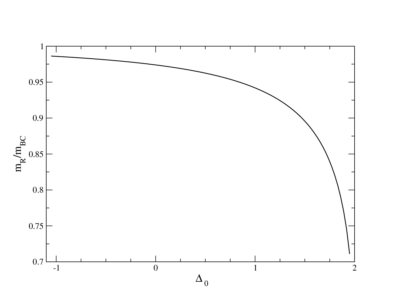
This analysis shows that corrections to critical temperatures are indeed small and are of order higher than . A further analysis should be carry out to obtain a finite shift by considering more complex diagrams. It is also supported by analytical values of which are close to numerical results reported in figure 1.
4 Extension to other spin-S models: generalization of the bare mass
The previous bare mass computed in the BC model, , allowed us to obtain a precise description of the second-order critical line in the phase diagram. This was obtained by taking the limit of low momentum in the effective action, see (30). This can be generalized for any value of the spin , in particular for higher values of . The equations obtained in section 2, equations (16) and (17), are general for they represent the fermionization of any spins-S model.
The construction of the fermionic action is however not an easy task, unlike the BC model which is a simpler case, but we expect to be able to extract a bare mass associated to non kinetic terms, or term involving derivatives with respect with space variables. At first approximation, we assume that the partition function and the free energy are singular in the low momentum limit when this bare mass vanishes. In the continuum limit, the ’s coefficients defined by relations (13) can be rewritten using formal derivatives, such as , etc… The derivatives contribute only to the kinetic energy and not to the bare mass. Keeping the first terms of the expansion, (as well as for the other coefficients ’s), the weights become uncoupled in the sense they contain variables depending only on local site and we define the mass as:
with and . The integral can be evaluated exactly by noticing for example that the arguments of the exponential can be combined with a that appears in some of the products to give a contribution . Indeed using the Grassmann integration rules and , we can write
Also a term can be combined with to give the same contribution. Since the are ordered, there are also signs to take into account and coming from the fact the variables have to be moved in the correct order before integration. We obtain after some algebra the general relation
| (51) |
where we have define the following quantities with initial condition ,
| (52) |
and if and are both even, and otherwise. We can apply this result to different cases to check the validity of this relation. For the Ising model () and , we obtain , or
| (53) |
which vanishes at the Ising critical temperature or with the normalization , which is independent, as expected, of . For the Blume-Capel model () we have , or more explicitly
| (54) |
This mass is directly proportionnal to the mass found in the previous section. Indeed, we have the relation
| (55) |
and therefore both masses vanish on the same line of critical points. The coefficient comes from a global rescaling of the Grassmann variables in the original weights which leads to the coefficient in the BC function partition (19) and (22), instead of the coefficient in front of (17). For we find in particular that (see table 1).
| Spin S | ||||
|---|---|---|---|---|
| 1 | 2 | 5 | 6 | |
| Refs. | [25] | [26], [19] | [27, 25, 28] | [25] |
| [25], [27] | ||||
| Spin S | ||||
| 11 | 12 | |||
| Refs. | [25] | [25] | [25, 29] |
The other masses are deduced by iteration of formula (51) and (52). For higher values of spin , we find:
| (56) |
For general spin , we can extend the previous results to the formula
| (57) |
This is a simple result giving a precise location of the second-order critical lines by solving the equation of the bare mass . We give for comparison tabulated values of at in table 1 for different values of , and references to numerical results (Monte-Carlo simulations, high-temperature expansions) given in the literature. In general, the agreement is good up to in most cases. For half-integer values of , the models possess an asymptote in the plane. Indeed, for for example, the equation given in (56) predicts the solution
| (58) |
which is bounded by below which there is no continuation of the second-order critical line. In the limit of large integer , the model defined in equation (1) is described by a continuous variable and is called continuous Ising model. We can still obtain a finite value of the critical line by taking the asymptotic value of equation (57)
| (59) |
and in particular for , we have the following expansion for large
| (60) |
with . We observe that the rescaled mass vanishes in this case when , in good agreement with numerical works for this model [25, 29], and it is worth noting that equation (59) also possesses a non trivial solution at which is simply given by . This value is different from the value expected for all finite models [8]. It can be suggested that there also exists a tricritical point before this non physical value is reached.
5 Conclusion
In this review paper, we have presented a method which tries to operate a correspondence between classical spin models and fermionic systems. We have extended Plecho’s method [6, 10] based on Ising model to generalized spin-S systems. The method is based on the projection onto polynomial components, depending specifically on the value of spin , of Boltzmann local weights given by equation (2). Then the introduction of pairs of Grassmann variables per site and the use of special symmetries such as mirror and associative symmetries in 2D for Grassmannian objects allows us to perform exactly the sum over the spin variables. This gives a representation of spin-S models in term of fermionic multiple integrals (17). Effective actions can in principle be deduced from this representation. We have shown that such action can be built exactly for the Blume Capel model (30) and the bare mass (35) gives accurate description of the second-order critical line. We have seen that there is no shift of this mass due to the effect of quartic potential of the effective theory at the lowest order expansion in the coupling parameter , implying that corrections to the critical temperature may be indeed small. This quartic potential is however responsible for the presence of a tricritical point, rendering the second order line instable by changing the sign of the stiffness coefficient or making the free-fermion spectrum itself instable. For general spin-S model, the bare mass can also be generalized and calculated directly in the low momentum limit (51) without knowing the full effective action, and still gives accurate description of second-order critical points even in the limit of the continuous Ising model.
References
- 1. E.H. Lieb, T.D. Schultz, and D.C. Mattis, Ann. Phys, 1961,16, 407.
- 2. T.D. Schultz, D.C. Mattis, and E.H. Lieb, Rev. Mod. Phys., 1964,36, 856.
- 3. P. Jordan and E. Wigner, Z. Phys., 1928 47, 631.
- 4. M.E. Fisher, J. Math. Phys. 1966, 7, 1776.
- 5. A.I. Bugrij in Electron-Electron Correlation Effects in Low-Dimentional Conductors and Superconductors. Editors: A.A. Ovchinnikov and I.I. Ukrainskii, Heidelberg, Springer-Verlag, 1991, 135-151.
- 6. V.N. Plechko, Theoretical and Mathematical Physics,1985, 64, 748-756.
- 7. K. Nojima, Int. J. Mod. Phys. B, 1998, 12, 1995.
- 8. J.-Y. Fortin and M. Clusel, Phys. Rev. B, 2008, 78,172402.
- 9. M. Blume, V.J. Emery, and R.B. Griffiths, Phys. Rev. A,1971, 4, 1071.
- 10. V.N. Plechko, Sov. Phys. Doklady, 1985, 30, 271.
- 11. M. Clusel, J.-Y. Fortin, and V.N. Plechko, J. Phys. A:Math. Theor., 2008, 41, 405004.
- 12. F.A. Berezin, The Method of second quantization, Academic Press, 1966.
- 13. T.M. Liaw, M.C. Huang, S.C. Lin, and M.C. Wu, Phys. Rev. B, 1999, 60, 12994.
- 14. M.C. Wu and C.K. Hu, J. Phys. A: Math. Gen., 2002 35, 5189.
- 15. M.B. Barbaro, A. Molinari, and F. Palumbo, Nucl. Phys. B, 1997, 487, 492.
- 16. V.N. Plechko, Anticommuting integrals and fermionic field theories for two-dimensional Ising models. A talk given at the VII International Conference on Symmetry Methods in Physics, ICSMP-95, Dubna, July 10-16, 1995. See also hep-th/9607053.
- 17. V.N. Plechko, Phys. Lett. A, 1998, 239, 289.
- 18. V.N. Plechko, J. Phys. Studies, 1999, 3, 312.
- 19. R. da Silva, Roberto, N.A. Alves, and J.R. Drugowich de Felício, Phys. Rev. E, 2002, 66, 026130.
- 20. C.J. Silva, A.A. Caparica, and J.A. Plascak, Phys. Rev. E, 2006, 73, 036702.
- 21. J.C. Xavier, F.C. Alcaraz, D. Pena Lara, and J.A. Plascak, Phys. Rev. B, 1998, 57, 11575.
- 22. P.D. Beale, Phys. Rev. B, 1986, 33, 1717.
- 23. Richard D. Mattuck, A Guide to Feynman Diagrams in the Many-body Problem, Courier Dover Publications, 1992.
- 24. A.M. Tsvelik, Quantum Field Theory in Condensed Matter Physics, Cambridge, 1995.
- 25. P. Butera, M. Comi, and A.J. Guttmann, Phys. Rev. B, 2003, 67, 054402.
- 26. P.F. Fox and A.J. Guttmann, J. Phys. C, 1973, 6, 913.
- 27. J.C. Xavier, F.C. Alcaraz, D.P. Lara, and J.A. Plascak, Phys. Rev. B, 1998, 57, 11575.
- 28. B.C.S. Grandi and W. Figueiredo, Phys. Rev. E, 2004, 70, 056109.
- 29. P. Bialas, P. Blanchard, S. Fortunato, D. Gandolfo, and H. Satz, Nucl. Phys. B, 2000, 583, 368.