跳到论文正文
W Papers独立论文阅读器 arXiv:0905.0884 论文正文 计算阅读时间 · 0%
引用这篇论文根据当前论文元数据生成,正式投稿前建议核对。


License: arXiv.org perpetual non-exclusive license
arXiv:0905.0884v1 [math.ST] 06 May 2009

Adaptive Dantzig density estimation

K. Bertin ††thanks: Supported by Project PBCT 13 laboratorio ANESTOC and Project FONDECYT 1090285. Departamento de Estadística, CIMFAV, Universidad de Valparaíso, Avenida Gran Bretaña 1091, Valparaíso, Chile. Tel 0056-(0)32-2508324. Email: karine.bertin@uv.cl    E. Le Pennec ††thanks: Laboratoire de Probabilité et Modèles Aléatoires, Université Paris 7, 175 rue de Chevaleret, F-75013 Paris, France. Email: lepennec@math.jussieu.fr    V. Rivoirard ††thanks: Laboratoire de Mathématique, U.M.R. C.N.R.S. 8628, Université Paris Sud, 91405 Orsay Cedex, France and Département de Mathématiques et Applications, U.M.R. C.N.R.S. 8553, ENS-Paris, 45 Rue d’Ulm, 75230 Paris Cedex 05, France, Email: vincent.rivoirard@math.u-psud.fr
Abstract

This paper deals with the problem of density estimation. We aim at building an estimate of an unknown density as a linear combination of functions of a dictionary. Inspired by Candès and Tao’s approach, we propose an ℓ1\ell_{1}-minimization under an adaptive Dantzig constraint coming from sharp concentration inequalities. This allows to consider a wide class of dictionaries. Under local or global coherence assumptions, oracle inequalities are derived. These theoretical results are also proved to be valid for the natural Lasso estimate associated with our Dantzig procedure. Then, the issue of calibrating these procedures is studied from both theoretical and practical points of view. Finally, a numerical study shows the significant improvement obtained by our procedures when compared with other classical procedures.

Keywords : Calibration, Concentration inequalities, Dantzig estimate, Density estimation, Dictionary, Lasso estimate, Oracle inequalities, Sparsity.

AMS subject classification : 62G07, 62G05, 62G20

1 Introduction

Various estimation procedures based on l1l_{1} penalization (exemplified by the Dantzig procedure in [13] and the LASSO procedure in [28]) have extensively been studied recently. These procedures are computationally efficient as shown in [17, 24, 25], and thus are adapted to high-dimensional data. They have been widely used in regression models, but only the Lasso estimator has been studied in the density model (see [7, 10, 29]). Although we will mostly consider the Dantzig estimator in the density model for which no result exists so far, we recall some of the classical results obtained in different settings by procedures based on l1l_{1} penalization.

The Dantzig selector has been introduced by Candès and Tao [13] in the linear regression model. More precisely, given

Y=A​λ0+ε,Y=A\lambda_{0}+\varepsilon,

where Y∈ℝnY\in\mathbb{R}^{n}, AA is a nn by MM matrix, ε∈ℝn\varepsilon\in\mathbb{R}^{n} is the noise vector and λ0∈ℝM\lambda_{0}\in\mathbb{R}^{M} is the unknown regression parameter to estimate, the Dantzig estimator is defined by

λ^D=argminλ∈ℝM||λ||ℓ1 subject to ||AT(Aλ−Y)||ℓ∞≤η,\hat{\lambda}^{D}=\arg\min_{\lambda\in\mathbb{R}^{M}}|\!|\lambda|\!|_{\ell_{1}}\text{ subject to }|\!|A^{T}(A\lambda-Y)|\!|_{\ell_{\infty}}\leq\eta,

where ||⋅||ℓ∞|\!|\cdot|\!|_{\ell_{\infty}} is the sup-norm in ℝM\mathbb{R}^{M}, ||⋅||ℓ1|\!|\cdot|\!|_{\ell_{1}} is the ℓ1\ell_{1} norm in ℝM\mathbb{R}^{M}, and η\eta is a regularization parameter. A natural companion of this estimator is the Lasso procedure or more precisely its relaxed form

λ^L=arg⁡minλ∈ℝM​{12​‖A​λ−Y‖ℓ22+η||λ||ℓ1},\hat{\lambda}^{L}=\arg\min_{\lambda\in\mathbb{R}^{M}}\left\{\frac{1}{2}|\!|A\lambda-Y|\!|_{\ell_{2}}^{2}\ +\eta|\!|\lambda|\!|_{\ell_{1}}\right\},

where η\eta plays exactly the exact same role as for the Dantzig estimator. This ℓ1\ell_{1} penalized method is also called basis pursuit in signal processing (see [14, 15]).

Candès and Tao [13] have obtained a bound for the ℓ2\ell_{2} risk of the estimator λ^D\hat{\lambda}^{D}, with large probability, under a global condition on the matrix AA (the Restricted Isometry Property) and a sparsity assumption on λ0\lambda_{0}, even for M≥nM\geq n. Bickel et al. [3] have obtained oracle inequalities and bounds of the ℓp\ell_{p} loss for both estimators under weaker assumptions. Actually, Bickel et al. [3] deal with the non parametric regression framework in which one observes

Yi=f(xi)+ei,i=1,…,nY_{i}=f(x_{i})+e_{i},\quad i=1,\ldots,n

where ff is an unknown function while (xi)i=1,…,n(x_{i})_{i=1,\ldots,n} are known design points and (ei)i=1,…,n(e_{i})_{i=1,\ldots,n} is a noise vector. There is no intrinsic matrix AA in this problem but for any dictionary of functions Υ=(φm)m=1,…,M\Upsilon=(\varphi_{m})_{m=1,\ldots,M} one can search ff as a weighted sum fλf_{\lambda} of elements of Υ\Upsilon

fλ=∑m=1Mλm​φmf_{\lambda}=\sum_{m=1}^{M}\lambda_{m}\varphi_{m}

and introduce the matrix A=(φm​(xi))i,mA=(\varphi_{m}(x_{i}))_{i,m}, which summarizes the information on the dictionary and on the design. Notice that if there exists λ0\lambda_{0} such that f=fλ0f=f_{\lambda_{0}} then the model can be rewritten exactly as the classical linear model. However, if it is not the case and if a model bias exists, the Dantzig and Lasso procedures can be after all applied under similar assumptions on AA. Oracle inequalities are obtained for which approximation theory plays an important role in [3, 8, 9, 29].

Let us also mention that in various settings, under various assumptions on the matrix AA (or more precisely on the associated Gram matrix G=AT​AG=A^{T}A), properties of these estimators have been established for subset selection (see [11, 20, 22, 23, 30, 31]) and for prediction (see [3, 19, 20, 23, 32]).

1.1 Our goals and results

We consider in this paper the density estimation framework already studied for the Lasso estimate by Bunea et al [7, 10] and van de Geer [29]. Namely, our goal is to estimate f0f_{0}, an unknown density function, by using the observations of an nn-sample of variables X1,…,XnX_{1},\dots,X_{n} of density f0f_{0}. As in the non parametric regression setting, we introduce a dictionary of functions Υ=(φm)m=1,…,M\Upsilon=(\varphi_{m})_{m=1,\ldots,M}, and search again estimates of f0f_{0} as linear combinations fλf_{\lambda} of the dictionary functions. We rely on the Gram matrix associated with Υ\Upsilon and on the empirical scalar products of f0f_{0} with φm\varphi_{m}

β^m=1n​∑i=1nφm​(Xi).\hat{\beta}_{m}=\frac{1}{n}\sum_{i=1}^{n}\varphi_{m}(X_{i}).

The Dantzig estimate f^D\hat{f}^{D} is then obtained by minimizing ‖λ‖ℓ1|\!|\lambda|\!|_{\ell_{1}} over the set of parameters λ\lambda satisfying the adaptive Dantzig constraint:

∀m∈{1,….M},|(Gλ)m−β^m|≤ηγ,m\forall\,m\in\{1,\ldots.M\},\quad\ |(G\lambda)_{m}-\hat{\beta}_{m}|\leq\eta_{\gamma,m}

where for m∈{1,…,M}m\in\{1,\ldots,M\}, (G​λ)m(G\lambda)_{m} is the scalar product of fλf_{\lambda} with φm\varphi_{m},

ηγ,m=2​~​σm2​γ​log⁡Mn+2​‖φm‖∞​γ​log⁡M3​n,\eta_{\gamma,m}=\sqrt{\frac{2\tilde{}\sigma^{2}_{m}\gamma\log M}{n}}+\frac{2|\!|\varphi_{m}|\!|_{\infty}\gamma\log M}{3n},

~​σm2\tilde{}\sigma^{2}_{m} is a sharp estimate of the variance of ^​βm\hat{}\beta_{m} and γ\gamma is a constant to be chosen. Section 2 gives precise definitions and heuristics for using this constraint. We just mention here that ηγ,m\eta_{\gamma,m} comes from sharp concentration inequalities to give tight constraints. Our idea is that if f0f_{0} can be decomposed on Υ\Upsilon as

f0=∑m=1Mλ0,m​φm,f_{0}=\sum_{m=1}^{M}\lambda_{0,m}\varphi_{m},

then we force the set of feasible parameters λ\lambda to contain λ0\lambda_{0} with large probability and to be as small as possible. Significant improvements in practice are expected.

Our goals in this paper are mainly twofold. First, we aim at establishing sharp oracle inequalities under very mild assumptions on the dictionary. Our starting point is that most of the papers in the literature assume that the functions of the dictionary are bounded by a constant independent of MM and nn, which constitutes a strong limitation, in particular for dictionaries based on histograms or wavelets (see for instance [6], [7], [8], [9], [11] or [29]). Such assumptions on the functions of Υ\Upsilon will not be considered in our paper. Likewise, our methodology does not rely on the knowledge of ‖f0‖∞|\!|f_{0}|\!|_{\infty} that can even be infinite (as noticed by Birgé [4] for the study of the integrated 𝕃2\mathbb{L}_{2}-risk, most of the papers in the literature typically assume that the sup-norm of the unknown density is finite with a known or estimated bound for this quantity). Finally, let us mention that, in contrast with what Bunea et al [10] did, we obtain oracle inequalities with leading constant 1, and furthermore these are established under much weaker assumptions on the dictionary than in [10].

The second goal of this paper deals with the problem of calibrating the so-called Dantzig constant γ\gamma: how should this constant be chosen to obtain good results in both theory and practice? Most of the time, for Lasso-type estimators, the regularization parameter is of the form a​log⁡Mna\sqrt{\frac{\log M}{n}} with aa a positive constant (see [3], [7], [6], [9], [12], [20] or [23] for instance). These results are obtained with large probability that depends on the tuning coefficient aa. In practice, it is not simple to calibrate the constant aa. Unfortunately, most of the time, the theoretical choice of the regularization parameter is not suitable for practical issues. This fact is true for Lasso-type estimates but also for many algorithms for which the regularization parameter provided by the theory is often too conservative for practical purposes (see [18] who clearly explains and illustrates this point for their thresholding procedure). So, one of the main goals of this paper is to fill the gap between the optimal parameter choice provided by theoretical results on the one hand and by a simulation study on the other hand. Only a few papers are devoted to this problem. In the model selection setting, the issue of calibration has been addressed by Birgé and Massart [5] who considered ℓ0\ell_{0}-penalized estimators in a Gaussian homoscedastic regression framework and showed that there exists a minimal penalty in the sense that taking smaller penalties leads to inconsistent estimation procedures. Arlot and Massart [1] generalized these results for non-Gaussian or heteroscedastic data and Reynaud-Bouret and Rivoirard [26] addressed this question for thresholding rules in the Poisson intensity framework.

Now, let us describe our results. By using the previous data-driven Dantzig constraint, oracle inequalities are derived under local conditions on the dictionary that are valid under classical assumptions on the structure of the dictionary. We extensively discuss these assumptions and we show their own interest in the context of the paper. Each term of these oracle inequalities is easily interpretable. Classical results are recovered when we further assume:

‖φm‖∞2≤c1​(nlog⁡M)​‖f0‖∞,|\!|\varphi_{m}|\!|_{\infty}^{2}\leq c_{1}\left(\frac{n}{\log M}\right)|\!|f_{0}|\!|_{\infty}~,

where c1c_{1} is a constant. This assumption is very mild and, unlike in classical works, allows to consider dictionaries based on wavelets. Then, relying on our Dantzig estimate, we build an adaptive Lasso procedure whose oracle performances are similar. This illustrates the closeness between Lasso and Dantzig-type estimates.

Our results are proved for γ>1\gamma>1. For the theoretical calibration issue, we study the performance of our procedure when γ<1\gamma<1. We show that in a simple framework, estimation of the straightforward signal f0=𝟏[0,1]f_{0}=\mathbf{1}_{[0,1]} cannot be performed at a convenient rate of convergence when γ<1\gamma<1. This result proves that the assumption γ>1\gamma>1 is thus not too conservative.

Finally, a simulation study illustrates how dictionary-based methods outperform classical ones. More precisely, we show that our Dantzig and Lasso procedures with γ>1\gamma>1, but close to 1, outperform classical ones, such as simple histogram procedures, wavelet thresholding or Dantzig procedures based on the knowledge of ‖f0‖∞|\!|f_{0}|\!|_{\infty} and less tight Dantzig constraints.

1.2 Outlines

Section 2 introduces the density estimator of f0f_{0} whose theoretical performances are studied in Section 3. Section 4 studies the Lasso estimate proposed in this paper. The calibration issue is studied in Section 5.1 and numerical experiments are performed in Section 5.2. Finally, Section 6 is devoted to the proofs of our results.

2 The Dantzig estimator of the density f0f_{0}

As said in Introduction, our goal is to build an estimate of f0f_{0} as a linear combination of functions of Υ=(φm)m=1,…,M\Upsilon=(\varphi_{m})_{m=1,\ldots,M}, where we assume without any loss of generality that, for any mm, ‖φm‖2=1\|\varphi_{m}\|_{2}=~1:

fλ=∑m=1Mλm​φm.f_{\lambda}=\sum_{m=1}^{M}\lambda_{m}\varphi_{m}.

For this purpose, we naturally rely on natural estimates of the 𝕃2\mathbb{L}_{2}-scalar products between f0f_{0} and the φm\varphi_{m}’s. So, for m∈{1,…,M}m\in\{1,\ldots,M\}, we set

β0,m=∫φm​(x)​f0​(x)​𝑑x,\beta_{0,m}=\int\varphi_{m}(x)f_{0}(x)dx, (1)

and we consider its empirical counterpart

β^m=1n​∑i=1nφm​(Xi)\hat{\beta}_{m}=\frac{1}{n}\sum_{i=1}^{n}\varphi_{m}(X_{i}) (2)

that is an unbiased estimate of β0,m\beta_{0,m}. The variance of this estimate is Var⁡(β^m)=σ0,m2n\mathrm{Var}(\hat{\beta}_{m})=\frac{\sigma_{0,m}^{2}}{n} where

σ0,m2=∫φm2​(x)​f0​(x)​𝑑x−β0,m2.\sigma_{0,m}^{2}=\int\varphi_{m}^{2}(x)f_{0}(x)dx-\beta_{0,m}^{2}. (3)

Note also that for any λ\lambda and any mm, the 𝕃2\mathbb{L}_{2}-scalar product between fλf_{\lambda} and φm\varphi_{m} can be easily computed:

∫φm​(x)​fλ​(x)​𝑑x=∑m′=1Mλm′​∫φm′​(x)​φm​(x)​𝑑x=(G​λ)m\int\varphi_{m}(x)f_{\lambda}(x)dx=\sum_{m^{\prime}=1}^{M}\lambda_{m^{\prime}}\int\varphi_{m^{\prime}}(x)\varphi_{m}(x)dx=(G\lambda)_{m}

where GG is the Gram matrix associated to the dictionary Υ\Upsilon defined for any 1≤m,m′≤M1\leq m,m^{\prime}\leq M by

Gm,m′=∫φm​(x)​φm′​(x)​𝑑x.G_{m,m^{\prime}}=\int\varphi_{m}(x)\varphi_{m^{\prime}}(x)dx.

Any reasonable choice of λ\lambda should ensure that the coefficients (G​λ)m(G\lambda)_{m} are close to β^m\hat{\beta}_{m} for all mm. Therefore, using Candès and Tao’s approach, we define the Dantzig constraint:

∀m∈{1,….M},|(Gλ)m−β^m|≤ηγ,m\forall\,m\in\{1,\ldots.M\},\quad\ |(G\lambda)_{m}-\hat{\beta}_{m}|\leq\eta_{\gamma,m} (4)

and the Dantzig estimate f^D\hat{f}^{D} by f^D=fλ^D,γ\hat{f}^{D}=f_{\hat{\lambda}^{D,\gamma}} with

λ^D,γ=argminλ∈ℝM||λ||ℓ1such that λ satisfies the Dantzig constraint (4),\hat{\lambda}^{D,\gamma}=\mathrm{argmin}_{\lambda\in\mathbb{R}^{M}}|\!|\lambda|\!|_{\ell_{1}}\quad\mbox{such that $\lambda$ satisfies the Dantzig constraint (\ref{constraint})},

where for γ>0\gamma>0 and m∈{1,…,M}m\in\{1,\ldots,M\},

ηγ,m=2​~​σm2​γ​log⁡Mn+2​‖φm‖∞​γ​log⁡M3​n,\eta_{\gamma,m}=\sqrt{\frac{2\tilde{}\sigma^{2}_{m}\gamma\log M}{n}}+\frac{2|\!|\varphi_{m}|\!|_{\infty}\gamma\log M}{3n}, (5)

with

~​σm2=^​σm2+2​‖φm‖∞​2​^​σm2​γ​log⁡Mn+8​‖φm‖∞2​γ​log⁡Mn\tilde{}\sigma^{2}_{m}=\hat{}\sigma^{2}_{m}+2|\!|\varphi_{m}|\!|_{\infty}\sqrt{\frac{2\hat{}\sigma^{2}_{m}\gamma\log M}{n}}+\frac{8|\!|\varphi_{m}|\!|_{\infty}^{2}\gamma\log M}{n} (6)

and

^​σm2=1n⁡(n−1)​∑i=2n∑j=1i−1(φm​(Xi)−φm​(Xj))2.\hat{}\sigma^{2}_{m}=\frac{1}{n(n-1)}\sum_{i=2}^{n}\sum_{j=1}^{i-1}(\varphi_{m}(X_{i})-\varphi_{m}(X_{j}))^{2}. (7)

Note that ηγ,m\eta_{\gamma,m} depends on the data, so the constraint (4) will be referred as the adaptive Dantzig constraint in the sequel. We now justify the introduction of the density estimate f^D\hat{f}^{D}.

The definition of ηλ,γ\eta_{\lambda,\gamma} is based on the following heuristics. Given mm, when there exists a constant c0>0c_{0}>0 such that f0​(x)≥c0f_{0}(x)\geq c_{0} for xx in the support of φm\varphi_{m} satisfying ‖φm‖∞2=on​(n​(log⁡M)−1)\|\varphi_{m}\|_{\infty}^{2}=o_{n}(n(\log M)^{-1}), then, with large probability, the deterministic term of (5) is negligible with respect to the random one. In this case, the random term is the main one and we asymptotically derive

ηγ,m≈2​γ​log⁡M​σ~m2n.\eta_{\gamma,m}\approx\sqrt{2\gamma\,{\log}M\,\frac{{\tilde{\sigma}}^{2}_{m}}{n}}. (8)

Having in mind that σ~m2/n{\tilde{\sigma}}^{2}_{m}/n is a convenient estimate for Var⁡(β^m)\mathrm{Var}(\hat{\beta}_{m}) (see the proof of Theorem 1), the shape of the right hand term of the formula (8) looks like the bound proposed by Candès and Tao [13] to define the Dantzig constraint in the linear model. Actually, the deterministic term of (5) allows to get sharp concentration inequalities. As often done in the literature, instead of estimating Var⁡(β^m)\mathrm{Var}(\hat{\beta}_{m}), we could use the inequality

Var⁡(β^m)=σ0,m2n≤‖f0‖∞n\mathrm{Var}(\hat{\beta}_{m})=\frac{{\sigma}^{2}_{0,m}}{n}\leq\frac{|\!|f_{0}|\!|_{\infty}}{n}

and we could replace σ~m2{\tilde{\sigma}}^{2}_{m} with ‖f0‖∞|\!|f_{0}|\!|_{\infty} in the definition of the ηγ,m\eta_{\gamma,m}. But this requires a strong assumption: f0f_{0} is bounded and ‖f0‖∞|\!|f_{0}|\!|_{\infty} is known. In our paper, Var⁡(β^m)\mathrm{Var}(\hat{\beta}_{m}) is estimated, which allows not to impose these conditions. More precisely, we slightly overestimate σ0,m2\sigma^{2}_{0,m} to control large deviation terms and this is the reason why we introduce σ~m2{\tilde{\sigma}}^{2}_{m} instead of using ^​σm2\hat{}\sigma^{2}_{m}, an unbiased estimate of σ0,m2\sigma_{0,m}^{2}. Finally, γ\gamma is a constant that has to to be suitably calibrated and plays a capital role in practice.

The following result justifies previous heuristics by showing that, if γ>1\gamma>1, with high probability, the quantity |β^m−β0,m||\hat{\beta}_{m}-\beta_{0,m}| is smaller than ηγ,m\eta_{\gamma,m} for all mm. The parameter ηγ,m\eta_{\gamma,m} with γ\gamma close to 11 can be viewed as the “smallest” quantity that ensures this property.

Theorem 1.

Let us assume that MM satisfies

n≤M≤exp⁡(nδ)n\leq M\leq\exp(n^{\delta}) (9)

for δ<1\delta<1. Let γ>1\gamma>1. Then, for any ε>0\varepsilon>0, there exists a constant C1​(ε,δ,γ)C_{1}(\varepsilon,\delta,\gamma) depending on ε,\varepsilon, δ\delta and γ\gamma such that

ℙ(∀m∈{1,…,M},|β0,m−β^m|≥ηγ,m)≤C1(ε,δ,γ)M1−γ1+ε.\mathbb{P}\left(\forall m\in\{1,\ldots,M\},\quad|\beta_{0,m}-\hat{\beta}_{m}|\geq\eta_{\gamma,m}\right)\leq C_{1}(\varepsilon,\delta,\gamma)M^{1-\frac{\gamma}{1+\varepsilon}}.

In addition, there exists a constant C2​(δ,γ)C_{2}(\delta,\gamma) depending on δ\delta and γ\gamma such that

ℙ(∀m∈{1,…,M},ηγ,m(−)≤ηγ,m≤ηγ,m(+))≤C2(δ,γ)M1−γ\mathbb{P}\left(\forall m\in\{1,\ldots,M\},\quad\eta^{(-)}_{\gamma,m}\leq\eta_{\gamma,m}\leq\eta^{(+)}_{\gamma,m}\right)\leq C_{2}(\delta,\gamma)M^{1-\gamma}

where, for m∈{1,…,M}m\in\{1,\ldots,M\},

ηγ,m(−)=σ0,m​8​γ​log⁡M7​n+2​‖φm‖∞​γ​log⁡M3​n\eta^{(-)}_{\gamma,m}=\sigma_{0,m}\sqrt{\frac{8\gamma\log M}{7n}}+\frac{2|\!|\varphi_{m}|\!|_{\infty}\gamma\log M}{3n}

and

ηγ,m(+)=σ0,m​16​γ​log⁡Mn+10​‖φm‖∞​γ​log⁡Mn.\eta^{(+)}_{\gamma,m}=\sigma_{0,m}\sqrt{\frac{16\gamma\log M}{n}}+\frac{10|\!|\varphi_{m}|\!|_{\infty}\gamma\log M}{n}.

This result is proved in Section 6.1. The first part is a sharp concentration inequality proved by using Bernstein type controls. The second part of the theorem proves that, up to constants depending on γ\gamma, ηγ,m\eta_{\gamma,m} is of order σ0,m​log⁡Mn+‖φm‖∞​log⁡Mn\sigma_{0,m}\sqrt{\frac{\log M}{n}}+|\!|\varphi_{m}|\!|_{\infty}\frac{\log M}{n} with high probability. Note that the assumption γ>1\gamma>1 is essential to obtain probabilities going to 0.

Finally, let λ0=(λ0,m)m=1,…,M∈ℝM\lambda_{0}=(\lambda_{0,m})_{m=1,\dots,M}\in\mathbb{R}^{M} such that

PΥ​f0=∑m=1Mλ0,m​φmP_{\Upsilon}f_{0}=\sum_{m=1}^{M}\lambda_{0,m}\varphi_{m}

where PΥP_{\Upsilon} is the projection on the space spanned by Υ\Upsilon. We have

(G​λ0)m=∫(PΥ​f0)​φm=∫f0​φm=β0,m.(G\lambda_{0})_{m}=\int(P_{\Upsilon}f_{0})\varphi_{m}=\int f_{0}\varphi_{m}=\beta_{0,m}.

So, Theorem 1 proves that λ0\lambda_{0} satisfies the adaptive Dantzig constraint (4) with probability larger than 1−C1​(ε,δ,γ)​M1−γ1+ε1-C_{1}(\varepsilon,\delta,\gamma)M^{1-\frac{\gamma}{1+\varepsilon}} for any ε>0\varepsilon>0. Actually, we force the set of parameters λ\lambda satisfying the adaptive Dantzig constraint to contain λ0\lambda_{0} with large probability and to be as small as possible. Therefore, f^D=fλ^D,γ\hat{f}^{D}=f_{\hat{\lambda}^{D,\gamma}} is a good candidate among sparse estimates linearly decomposed on Υ\Upsilon for estimating f0f_{0}.

We mention that Assumption (9) can be relaxed and we can take M<nM<n provided the definition of ηγ,m\eta_{\gamma,m} is modified.

3 Results for the Dantzig estimators

In the sequel, we will denote λ^D=λ^D,γ\hat{\lambda}^{D}=\hat{\lambda}^{D,\gamma} to simplify the notations, but the Dantzig estimator f^D\hat{f}^{D} still depends on γ\gamma. Moreover, we assume that (9) is true and we denote the vector ηγ=(ηγ,m)m=1,…,M\eta_{\gamma}=(\eta_{\gamma,m})_{m=1,\ldots,M} considered with the Dantzig constant γ>1\gamma>1.

3.1 The main result under local assumptions

Let us state the main result of this paper. For any J⊂{1,…,M}J\subset\{1,\dots,M\}, we set JC={1,…,M}∖JJ^{C}=\{1,\dots,M\}\smallsetminus J and define λJ\lambda_{J} the vector which has the same coordinates as λ\lambda on JJ and zero coordinates on JCJ^{C}. We introduce a local assumption indexed by a subset J0J_{0}.

  • •

    Local Assumption Given J0⊂{1,…,M}J_{0}\subset\{1,\dots,M\}, for some constants κJ0>0\kappa_{J_{0}}>0 and μJ0>0\mu_{J_{0}}>0 depending on J0J_{0}, we have for any λ\lambda,

    ‖fλ‖2≥κJ0​‖λJ0‖ℓ2−μJ0​(‖λJ0C‖ℓ1−||λJ0||ℓ1)+.|\!|f_{\lambda}|\!|_{2}\geq\kappa_{J_{0}}|\!|\lambda_{J_{0}}|\!|_{\ell_{2}}-\mu_{J_{0}}\left(|\!|\lambda_{J_{0}^{C}}|\!|_{\ell_{1}}-|\!|\lambda_{J_{0}}|\!|_{\ell_{1}}\right)_{+}. (L​A​(J0,κJ0,μJ0)LA(J_{0},\kappa_{J_{0}},\mu_{J_{0}}))

We obtain the following oracle type inequality without any assumption on f0f_{0}.

Theorem 2.

Let J0⊂{1,…,M}J_{0}\subset\{1,\ldots,M\} be fixed. We suppose that ( ⁢ L A ( J 0 , κ J 0 , μ J 0 ) ) holds. Then, with probability at least 1−C1​(ε,δ,γ)​M1−γ1+ε1-C_{1}(\varepsilon,\delta,\gamma)M^{1-\frac{\gamma}{1+\varepsilon}}, we have for any β>0\beta>0,

‖f^D−f0‖22≤infλ∈ℝM{‖fλ−f0‖22+β​Λ​(λ,J0c)2|J0|​(1+2​μJ0​|J0|κJ0)2+16​|J0|​(1β+1κJ02)​‖ηγ‖ℓ∞2},|\!|\hat{f}^{D}-f_{0}|\!|_{2}^{2}\leq\inf_{\lambda\in\mathbb{R}^{M}}\left\{|\!|f_{\lambda}-f_{0}|\!|_{2}^{2}+\beta\frac{\Lambda(\lambda,J_{0}^{c})^{2}}{|J_{0}|}\left(1+\frac{2\mu_{J_{0}}\sqrt{|J_{0}|}}{\kappa_{J_{0}}}\right)^{2}+16|J_{0}|\left(\frac{1}{\beta}+\frac{1}{\kappa_{J_{0}}^{2}}\right)|\!|\eta_{\gamma}|\!|_{\ell_{\infty}}^{2}\right\}, (10)

with

Λ⁡(λ,J0c)=‖λJ0C‖ℓ1+(‖λ^D‖ℓ1−‖λ‖ℓ1)+2.\Lambda(\lambda,J_{0}^{c})=|\!|\lambda_{J_{0}^{C}}|\!|_{\ell_{1}}+\frac{\left(|\!|\hat{\lambda}^{D}|\!|_{\ell_{1}}-|\!|\lambda|\!|_{\ell_{1}}\right)_{+}}{2}.

Let us comment each term of the right hand side of (10). The first term is an approximation term which measures the closeness between f0f_{0} and fλf_{\lambda}. This term can vanish if f0f_{0} can be decomposed on the dictionary. The second term is a price to pay when either λ\lambda is not supported by the subset J0J_{0} considered or it does not satisfy the condition ‖λ^D‖ℓ1≤‖λ‖ℓ1|\!|\hat{\lambda}^{D}|\!|_{\ell_{1}}\leq|\!|\lambda|\!|_{\ell_{1}} which holds as soon as λ\lambda satisfy the adaptive Dantzig constraint. Finally, the last term, which does not depend on λ\lambda, can be viewed as a variance term corresponding to the estimation on the subset J0J_{0}. Indeed, remember that ηγ,m\eta_{\gamma,m} relies on an estimate of the variance of ^​βm\hat{}\beta_{m}. Furthermore, we have with high probability:

‖ηγ‖ℓ∞2\displaystyle|\!|\eta_{\gamma}|\!|_{\ell_{\infty}}^{2} ≤\displaystyle\leq 2​(16​σ0,m2​γ​log⁡Mn+(10​‖φm‖∞​γ​log⁡Mn)2).\displaystyle 2\left(\frac{16\sigma_{0,m}^{2}\gamma\log M}{n}+\left(\frac{10|\!|\varphi_{m}|\!|_{\infty}\gamma\log M}{n}\right)^{2}\right).

So, if f0f_{0} is bounded then, σ0,m2≤‖f0‖∞\sigma_{0,m}^{2}\leq|\!|f_{0}|\!|_{\infty} and if there exists a constant c1c_{1} such that for any mm,

‖φm‖∞2≤c1​(nlog⁡M)​‖f0‖∞,|\!|\varphi_{m}|\!|_{\infty}^{2}\leq c_{1}\left(\frac{n}{\log M}\right)|\!|f_{0}|\!|_{\infty}, (11)

(which is true for instance for a bounded dictionary), then

‖ηγ‖ℓ∞2≤C​‖f0‖∞​log⁡Mn,|\!|\eta_{\gamma}|\!|_{\ell_{\infty}}^{2}\leq C|\!|f_{0}|\!|_{\infty}\frac{\log M}{n},

(where CC is a constant depending on γ\gamma and c1c_{1}) and tends to 0 when nn goes to ∞\infty. We obtain thus the following result.

Corollary 1.

Let J0⊂{1,…,M}J_{0}\subset\{1,\ldots,M\} be fixed. We suppose that ( ⁢ L A ( J 0 , κ J 0 , μ J 0 ) ) holds. If (11) is satisfied then, with probability at least 1−C1​(ε,δ,γ)​M1−γ1+ε1-C_{1}(\varepsilon,\delta,\gamma)M^{1-\frac{\gamma}{1+\varepsilon}}, we have for any β>0\beta>0, for any λ\lambda that satisfies the adaptive Dantzig constraint

‖f^D−f0‖22≤‖fλ−f0‖22+β​c2​(1+κJ0−2​μJ02​|J0|)​‖λJ0C‖ℓ12|J0|+c3​(β−1+κJ0−2)​|J0|||f0||∞​log⁡Mn,|\!|\hat{f}^{D}-f_{0}|\!|_{2}^{2}\leq|\!|f_{\lambda}-f_{0}|\!|_{2}^{2}+\beta c_{2}(1+\kappa_{J_{0}}^{-2}\mu_{J_{0}}^{2}|J_{0}|)\frac{|\!|\lambda_{J_{0}^{C}}|\!|_{\ell_{1}}^{2}}{|J_{0}|}+c_{3}(\beta^{-1}+\kappa_{J_{0}}^{-2})|J_{0}||\!|f_{0}|\!|_{\infty}\frac{\log M}{n}, (12)

where c2c_{2} is an absolute constant and c3c_{3} depends on c1c_{1} and γ\gamma.

The parameter β\beta calibrates the weights given for the bias and variance terms. Remark that if f0=fλ0f_{0}=f_{\lambda_{0}} and if ( ⁢ L A ( J 0 , κ J 0 , μ J 0 ) ) holds with J0=Jλ0J_{0}=J_{\lambda_{0}}, under (11), the proof of Theorem 2 yields the more classical inequality

‖f^D−f0‖22≤C′​|J0|​‖f0‖∞​log⁡Mn,|\!|\hat{f}^{D}-f_{0}|\!|_{2}^{2}\leq C^{\prime}|J_{0}||\!|f_{0}|\!|_{\infty}\frac{\log M}{n},

where C′=c3​κJ0−2C^{\prime}=c_{3}\kappa_{J_{0}}^{-2}, with at least the same probability 1−C1​(ε,δ,γ)​M1−γ1+ε1-C_{1}(\varepsilon,\delta,\gamma)M^{1-\frac{\gamma}{1+\varepsilon}}.

Assumption ( ⁢ L A ( J 0 , κ J 0 , μ J 0 ) ) is local, in the sense that the constants κJ0\kappa_{J_{0}} and μJ0\mu_{J_{0}} (or their mere existence) may highly depend on the subset J0J_{0}. For a given λ\lambda, the best choice for J0J_{0} in Inequalities (10) and (12) depends thus on the interaction between these constants and the value of λ\lambda itself. Note that the assumptions of Theorem 2 are reasonable as the next section gives conditions for which Assumption ( ⁢ L A ( J 0 , κ J 0 , μ J 0 ) ) holds simultaneously with the same constant κ\kappa and μ\mu for all subsets J0J_{0} of the same size.

3.2 Results under global assumptions

As usual, when M>nM>n, properties of the Dantzig estimate can be derived from assumptions on the structure of the dictionary Υ\Upsilon. For l∈ℕl\in\mathbb{N}, we denote

ϕmin​(l)\displaystyle\phi_{\min}(l) =min|J|≤l⁡minλ∈ℝMλJ≠0​‖fλJ‖22‖λJ‖ℓ22\displaystyle=\min_{|J|\leq l}\min_{\begin{subarray}{c}\lambda\in\mathbb{R}^{M}\\ \lambda_{J}\neq 0\end{subarray}}\frac{|\!|f_{\lambda_{J}}|\!|_{2}^{2}}{|\!|\lambda_{J}|\!|_{\ell_{2}}^{2}} and ϕmax​(l)\displaystyle\phi_{\max}(l) =max|J|≤l⁡maxλ∈ℝMλJ≠0​‖fλJ‖22‖λJ‖ℓ22.\displaystyle=\max_{|J|\leq l}\max_{\begin{subarray}{c}\lambda\in\mathbb{R}^{M}\\ \lambda_{J}\neq 0\end{subarray}}\frac{|\!|f_{\lambda_{J}}|\!|_{2}^{2}}{|\!|\lambda_{J}|\!|_{\ell_{2}}^{2}}.

These quantities correspond to the “restricted” eigenvalues of the Gram matrix GG. Assuming that ϕmin​(l)\phi_{\min}(l) and ϕmax​(l)\phi_{\max}(l) are close to 1 means that every set of columns of GG with cardinality less than ll behaves like an orthonormal system. We also consider the restricted correlations

θl,l′=max|J|≤l|J′|≤l′J∩J′=∅⁡maxλ,λ′∈ℝMλJ≠0,λJ′′≠0​⟨fλJ,fλJ′′⟩‖λJ‖ℓ2​‖λJ′′‖ℓ2.\theta_{l,l^{\prime}}=\max_{\begin{subarray}{c}\ |J|\leq l\\ \ |J^{\prime}|\leq l^{\prime}\\ J\cap J^{\prime}=\emptyset\end{subarray}}\max_{\begin{subarray}{c}\lambda,\lambda^{\prime}\in\mathbb{R}^{M}\\ \lambda_{J}\neq 0,\lambda^{\prime}_{J^{\prime}}\neq 0\end{subarray}}\frac{\langle f_{\lambda_{J}},f_{\lambda^{\prime}_{J^{\prime}}}\rangle}{|\!|\lambda_{J}|\!|_{\ell_{2}}|\!|\lambda^{\prime}_{J^{\prime}}|\!|_{\ell_{2}}}.

Small values of θl,l′\theta_{l,l^{\prime}} mean that two disjoint sets of columns of GG with cardinality less than ll and l′l^{\prime} span nearly orthogonal spaces. We will use one of the following assumptions considered in [3].

  • •

    Assumption 1 For some integer 1≤s≤M/21\leq s\leq M/2, we have

    ϕmin​(2​s)>θs,2​s.\phi_{\min}(2s)>\theta_{s,2s}. (A1(s))

    Oracle inequalities of the Dantzig selector were established under this assumption in the parametric linear model by Candès and Tao in [13]. It was also considered by Bunea, Ritov and Tsybakov [3] for non-parametric regression and for the Lasso estimate. The next assumption, proposed in [3], constitutes an alternative to Assumption 1.

  • •

    Assumption 2 For some integers ss and ll such that

    1≤s≤M2,l≥sands+l≤M,1\leq s\leq\frac{M}{2},\quad l\geq s\quad\mbox{and}\quad s+l\leq M, (13)

    we have

    l​ϕmin​(s+l)>s​ϕmax​(l).l\phi_{\min}(s+l)>s\phi_{\max}(l). (A2(s,l))

    If Assumption 2 is true for ss and ll such that l≫sl\gg s, then Assumption 2 means that ϕmin​(l)\phi_{\min}(l) cannot decrease at a rate faster than l−1l^{-1} and this condition is related to the “incoherent designs” condition stated in [23].

In the sequel, we set, under Assumption 1,

κ1​(s)=ϕmin​(2​s)​(1−θs,2​sϕmin​(2​s))>0,μ1​(s)=θs,2​ss​ϕmin​(2​s)\kappa_{1}(s)=\sqrt{\phi_{\min}(2s)}\left(1-\frac{\theta_{s,2s}}{\phi_{\min}(2s)}\right)>0,\quad\mu_{1}(s)=\frac{\theta_{s,2s}}{\sqrt{s\phi_{\min}(2s)}}

and under Assumption 2,

κ2​(s,l)=ϕmin​(s+l)​(1−s​ϕmax​(l)l​ϕmin​(s+l))>0,μ2​(s,l)=ϕmax​(l)l.\kappa_{2}(s,l)=\sqrt{\phi_{\min}(s+l)}\left(1-\sqrt{\frac{s\phi_{\max}(l)}{l\phi_{\min}(s+l)}}\right)>0,\quad\mu_{2}(s,l)=\sqrt{\frac{\phi_{\max}(l)}{l}}.

Now, to apply Theorem 2, we need to check ( ⁢ L A ( J 0 , κ J 0 , μ J 0 ) ) for some some subset J0J_{0} of {1,…,M}\{1,\ldots,M\}. Either Assumption 1 or Assumption 2 implies this assumption. Indeed, we have the following result.

Proposition 1.

Let ss and ll two integers satisfying (13). We suppose that (A1(s)) or (A2(s,l)) is true. Let J0⊂{1,…,M}J_{0}\subset\{1,\ldots,M\} of size |J0|=s|J_{0}|=s and λ∈ℝM\lambda\in\mathbb{R}^{M}, then we have

‖fλ‖2≥κ​‖λJ0‖ℓ2−μ​(‖λJ0C‖ℓ1−||λJ0||ℓ1)+|\!|f_{\lambda}|\!|_{2}\geq\kappa|\!|\lambda_{J_{0}}|\!|_{\ell_{2}}-\mu\left(|\!|\lambda_{J_{0}^{C}}|\!|_{\ell_{1}}-|\!|\lambda_{J_{0}}|\!|_{\ell_{1}}\right)_{+}

with κ=κ1​(s)\kappa=\kappa_{1}(s) and μ=μ1​(s)\mu=\mu_{1}(s) under (A1(s)) (respectively κ=κ2​(s,l)\kappa=\kappa_{2}(s,l) and μ=μ2​(s,l)\mu=\mu_{2}(s,l) under (A2(s,l)). If (A1(s)) and (A2(s,l)) are both satisfied, κ=max⁡(κ1​(s),κ2​(s,l))\kappa=\max(\kappa_{1}(s),\kappa_{2}(s,l)) and μ=min⁡(μ1​(s),μ2​(s,l))\mu=\min(\mu_{1}(s),\mu_{2}(s,l)).

Proposition 1 proves that Theorem 2 can be applied under Assumptions 1 or 2. In addition, the constants κJ0\kappa_{J_{0}} and μJ0\mu_{J_{0}} only depend on |J0||J_{0}|. From Theorem 2, we deduce the following result.

Theorem 3.

Let ss and ll two integers satisfying (13). We suppose that (A1(s)) or (A2(s,l)) is true. Then, with probability at least 1−C1​(ε,δ,γ)​M1−γ1+ε1-C_{1}(\varepsilon,\delta,\gamma)M^{1-\frac{\gamma}{1+\varepsilon}}, we have for any β>0\beta>0,

‖f^D−f0‖22≤infλ∈ℝMinfJ0⊂{1,…,M}|J0|=s{‖fλ−f0‖22+β​Λ​(λ,J0c)2s​(1+2​μ​sκ)2+16​s​(1β+1κ2)​‖ηγ‖ℓ∞2}|\!|\hat{f}^{D}-f_{0}|\!|_{2}^{2}\leq\inf_{\lambda\in\mathbb{R}^{M}}\inf_{\begin{subarray}{c}J_{0}\subset\{1,\ldots,M\}\\ |J_{0}|=s\end{subarray}}\left\{|\!|f_{\lambda}-f_{0}|\!|_{2}^{2}+\beta\frac{\Lambda(\lambda,J_{0}^{c})^{2}}{s}\left(1+\frac{2\mu\sqrt{s}}{\kappa}\right)^{2}+16s\left(\frac{1}{\beta}+\frac{1}{\kappa^{2}}\right)|\!|\eta_{\gamma}|\!|_{\ell_{\infty}}^{2}\right\}

where

Λ⁡(λ,J0c)=‖λJ0C‖ℓ1+(‖λ^D‖ℓ1−‖λ‖ℓ1)+2.\Lambda(\lambda,J_{0}^{c})=|\!|\lambda_{J_{0}^{C}}|\!|_{\ell_{1}}+\frac{\left(|\!|\hat{\lambda}^{D}|\!|_{\ell_{1}}-|\!|\lambda|\!|_{\ell_{1}}\right)_{+}}{2}.

Remark that the best subset J0J_{0} of cardinal ss in Theorem 3 can be easily chosen for a given λ\lambda: it is given by the set of the ss largest coordinates of λ\lambda. This was not necessarily the case in Theorem 2 for which a different subset may give a better local condition and then may provide a smaller bound. If we further assume the mild assumption (11) on the sup norm of the dictionary introduced in the previous section, we deduce the following result.

Corollary 2.

Let ss and ll two integers satisfying (13). We suppose that (A1(s)) or (A2(s,l)) is true. If (11) is satisfied, with probability at least 1−C1​(ε,δ,γ)​M1−γ1+ε1-C_{1}(\varepsilon,\delta,\gamma)M^{1-\frac{\gamma}{1+\varepsilon}}, we have for any β>0\beta>0, any λ\lambda that satisfies the adaptive Dantzig constraint and for the best subset J0J_{0} of cardinal ss (that corresponds to the ss largest coordinates of λ\lambda in absolute value),

‖f^D−f0‖22≤‖fλ−f0‖22+β​c2​(1+κ−2​μ2​s)​‖λJ0C‖ℓ12s+c3​(β−1+κ−2)​s||f0||∞​log⁡Mn,|\!|\hat{f}^{D}-f_{0}|\!|_{2}^{2}\leq|\!|f_{\lambda}-f_{0}|\!|_{2}^{2}+\beta c_{2}(1+\kappa^{-2}\mu^{2}s)\frac{|\!|\lambda_{J_{0}^{C}}|\!|_{\ell_{1}}^{2}}{s}+c_{3}(\beta^{-1}+\kappa^{-2})s|\!|f_{0}|\!|_{\infty}\frac{\log M}{n}, (14)

where c2c_{2} is an absolute constant and c3c_{3} depends on c1c_{1} and γ\gamma.

Note that, when λ\lambda is ss-sparse so that λJ0C=0\lambda_{J_{0}^{C}}=0, the oracle inequality (14) corresponds to the classical oracle inequality obtained in parametric frameworks (see [12] or [13] for instance) or in non-parametric settings. See, for instance [6], [7], [8], [9], [11] or [29] but in these works, the functions of the dictionary are assumed to be bounded by a constant independent of MM and nn. So, the adaptive Dantzig estimate requires weaker conditions since under (11), ‖φm‖∞|\!|\varphi_{m}|\!|_{\infty} can go to ∞\infty when nn grows. This point is capital for practical purposes, in particular when wavelet bases are considered.

4 Connections between the Dantzig and Lasso estimates

We show in this section the strong connections between Lasso and Dantzig estimates, which has already been illustrated in [3] for non-parametric regression models. By choosing convenient random weights depending on ηγ\eta_{\gamma} for ℓ1\ell_{1}-minimization, the Lasso estimate satisfies the adaptive Dantzig constraint. More precisely, we consider the Lasso estimator given by the solution of the following minimization problem

λ^L,γ=argminλ∈ℝM​{R⁡(λ)+2​∑m=1Mηγ,m​|λm|},\hat{\lambda}^{L,\gamma}=\mathrm{argmin}_{\lambda\in\mathbb{R}^{M}}\left\{R(\lambda)+2\sum_{m=1}^{M}\eta_{\gamma,m}|\lambda_{m}|\right\}, (15)

where

R⁡(λ)=‖fλ‖22−2n​∑i=1nfλ​(Xi).R(\lambda)=|\!|f_{\lambda}|\!|_{2}^{2}-\frac{2}{n}\sum_{i=1}^{n}f_{\lambda}(X_{i}).

Note that R⁡(⋅)R(\cdot) is the quantity minimized in unbiased estimation of the risk. For simplifications, we write λ^L=λ^L,γ\hat{\lambda}^{L}=\hat{\lambda}^{L,\gamma}. We denote f^L=fλ^L\hat{f}^{L}=f_{\hat{\lambda}^{L}}. As said in Introduction, classical Lasso estimates are defined as the minimizer of expressions of the form

{R⁡(λ)+2​η​∑m=1M|λm|},\left\{R(\lambda)+2\eta\sum_{m=1}^{M}|\lambda_{m}|\right\},

where η\eta is proportional to log⁡Mn\sqrt{\frac{\log M}{n}}. So, λ^L\hat{\lambda}^{L} appears as a data-driven version of classical Lasso estimates.

The first order condition for the minimization of the expression given in (15) corresponds exactly to the adaptive Dantzig constraint and thus Theorem 3 always applies to λ^L\hat{\lambda}^{L}. Working along the lines of the proof of Theorem 3 (Replace fλf_{\lambda} by f^D\hat{f}^{D} and f^D\hat{f}^{D} by f^L\hat{f}^{L} in (26) and (27)), one can prove a slightly stronger result.

Theorem 4.

Let us assume that assumptions of Theorem 3 are true. Let J0⊂{1,…,M}J_{0}\subset\{1,\ldots,M\} of size |J0|=s|J_{0}|=s. Then, with probability at least 1−C1​(ε,δ,γ)​M1−γ1+ε1-C_{1}(\varepsilon,\delta,\gamma)M^{1-\frac{\gamma}{1+\varepsilon}}, we have for any β>0\beta>0,

|‖f^D−f0‖22−‖f^L−f0‖22|≤β​‖λ^J0CL‖ℓ12s​(1+2​μ​sκ)2+16​s​(1β+1κ2)​‖ηγ‖ℓ∞2.\left||\!|\hat{f}^{D}-f_{0}|\!|_{2}^{2}-|\!|\hat{f}^{L}-f_{0}|\!|_{2}^{2}\right|\leq\beta\frac{|\!|\hat{\lambda}^{L}_{J_{0}^{C}}|\!|_{\ell_{1}}^{2}}{s}\left(1+\frac{2\mu\sqrt{s}}{\kappa}\right)^{2}+16s\left(\frac{1}{\beta}+\frac{1}{\kappa^{2}}\right)|\!|\eta_{\gamma}|\!|_{\ell_{\infty}}^{2}.

To extend this theoretical result, numerical performances of the Dantzig and Lasso estimates will be compared in Section 5.2.

5 Calibration and numerical experiments

5.1 The calibration issue

In this section, we consider the problem of calibrating previous estimates. In particular, we prove that the sufficient condition γ>1\gamma>1 is “almost” a necessary condition since we derive a special and very simple framework in which Lasso and Dantzig estimates cannot achieve the optimal rate if γ<1\gamma<1 (“almost” means that the case γ=1\gamma=1 remains an open question). Let us describe this simple framework. The dictionary Υ\Upsilon considered in this section is the orthonormal Haar system:

Υ={ϕj​k:−1≤j≤j0, 0≤k<2j},\Upsilon=\left\{\phi_{jk}:\quad-1\leq j\leq j_{0},\ 0\leq k<2^{j}\right\},

with ϕ−10=𝟏[0,1]\phi_{-10}=\mathbf{1}_{[0,1]}, 2j0+1=n2^{j_{0}+1}=n, and for 0≤j≤j0,0\leq j\leq j_{0}, 0≤k≤2j−10\leq k\leq 2^{j}-1,

ϕj​k=2j/2​(1[k/2j,(k+0.5)/2j]−1[(k+0.5)/2j,(k+1)/2j]).\phi_{jk}=2^{j/2}\left(1_{[k/2^{j},(k+0.5)/2^{j}]}-1_{[(k+0.5)/2^{j},(k+1)/2^{j}]}\right).

In this case, M=nM=n. In this setting, since functions of Υ\Upsilon are orthonormal, the Gram matrix GG is the identity. Thus, the Lasso and Dantzig estimates both correspond to the soft thresholding rule:

f^D=f^L=∑m=1Msign(β^m)(|β^m|−ηγ,m)1{|β^m|>ηγ,m}φm.\hat{f}^{D}=\hat{f}^{L}=\sum_{m=1}^{M}\mbox{sign}(\hat{\beta}_{m})\left(|\hat{\beta}_{m}|-\eta_{\gamma,m}\right)1_{\{|\hat{\beta}_{m}|>\eta_{\gamma,m}\}}\varphi_{m}.

Now, our goal is to estimate f0=ϕ−10=𝟏[0,1]f_{0}=\phi_{-10}=\mathbf{1}_{[0,1]} by using f^D\hat{f}^{D} depending on γ\gamma and to show the influence of this constant. Unlike previous results stated in probability, we consider the expectation of the 𝕃2\mathbb{L}_{2}-risk:

Theorem 5.

On the one hand, if γ>1\gamma>1, there exists a constant CC such that

𝔼​‖f^D−f0‖22≤C​log⁡nn,\mathbb{E}|\!|\hat{f}^{D}-f_{0}|\!|_{2}^{2}\leq\frac{C\log n}{n}, (16)

On the other hand, if γ<1\gamma<1, there exists a constant cc and δ<1\delta<1 such that

𝔼​‖f^D−f0‖22≥cnδ.\mathbb{E}|\!|\hat{f}^{D}-f_{0}|\!|^{2}_{2}\geq\frac{c}{n^{\delta}}. (17)

This result shows that choosing γ<1\gamma<1 is a bad choice in our setting. Indeed, in this case, the Lasso and Dantzig estimates cannot estimate a very simple signal (f0=𝟏[0,1]f_{0}=\mathbf{1}_{[0,1]}) at a convenient rate of convergence.

Refer to caption
Figure 1: Graphs of γ↦log2⁡(Rn¯​(γ))\gamma\mapsto\log_{2}(\overline{R_{n}}(\gamma)) for n=2Jn=2^{J} with, from top to bottom, J=4,5,6,…,13J=4,5,6,\ldots,13

A small simulation study is carried out to strengthen this theoretical asymptotic result. Performing our estimation procedure 100 times, we compute the average risk Rn¯​(γ)\overline{R_{n}}(\gamma) for several values of the Dantzig constant γ\gamma and several values of nn. This computation is summarized in Figure 1 which displays the logarithm of Rn¯​(γ)\overline{R_{n}}(\gamma) for n=2Jn=2^{J} with, from top to bottom, J=4,5,6,…,13J=4,5,6,\ldots,13 on a grid of γ\gamma’s around 11. To discuss our results, we denote by γmin​(n)\gamma_{\min}(n) the best γ\gamma: γmin​(n)=argminγ>0​Rn¯​(γ).\gamma_{\min}(n)=\mathrm{argmin}_{\gamma>0}\overline{R_{n}}(\gamma). We note that 1/2≤γmin​(n)≤11/2\leq\gamma_{\min}(n)\leq 1 for all values of nn, with γmin​(n)\gamma_{\min}(n) getting closer to 11 as nn increases. Taking γ\gamma too small strongly deteriorates the performance while a value close to 11 ensures a risk withing a factor 22 of the optimal risk. The assumption γ>1\gamma>1 giving a theoretical control on the quadratic error is thus not too conservative. Following these results, we set γ=1.01\gamma=1.01 in our numerical experiments in the next subsection.

5.2 Numerical experiments

In this section, we present our numerical experiments with the Dantzig density estimator and their results. We test our estimator with a collection of 6 dictionaries, 4 densities described below and for 2 sample sizes. We compare our procedure with the adaptive Lasso introduced in Section 4 and with a non adaptive Dantzig estimator. We also consider a two-step estimation procedure, proposed by Candès and Tao [13], which improves the numerical results.

The numerical scheme for a given dictionary Υ=(φm)m=1,…,M\Upsilon=(\varphi_{m})_{m=1,\ldots,M} and a sample (Xi)i=1,…,n(X_{i})_{i=1,\ldots,n} is the following.

  1. 1.

    Compute β^m\hat{\beta}_{m} for all mm,

  2. 2.

    Compute σ^m2\hat{\sigma}^{2}_{m},

  3. 3.

    Compute ηγ,m\eta_{\gamma,m} as defined in (5) by

    ηγ,m=2​~​σm2​γ​log⁡Mn+2​‖φm‖∞​γ​log⁡M3​n,\eta_{\gamma,m}=\sqrt{\frac{2\tilde{}\sigma^{2}_{m}\gamma\log M}{n}}+\frac{2|\!|\varphi_{m}|\!|_{\infty}\gamma\log M}{3n},

    with

    ~​σm2=^​σm2+2​‖φm‖∞​2​^​σm2​γ​log⁡Mn+8​‖φm‖∞2​γ​log⁡Mn\tilde{}\sigma^{2}_{m}=\hat{}\sigma^{2}_{m}+2|\!|\varphi_{m}|\!|_{\infty}\sqrt{\frac{2\hat{}\sigma^{2}_{m}\gamma\log M}{n}}+\frac{8|\!|\varphi_{m}|\!|_{\infty}^{2}\gamma\log M}{n}

    and γ=1.01\gamma=1.01.

  4. 4.

    Compute the coefficients λ^D,γ\hat{\lambda}^{D,\gamma} of the Dantzig estimate, λ^D,γ=argminλ∈ℝM​‖λ‖ℓ1\hat{\lambda}^{D,\gamma}=\mathrm{argmin}_{\lambda\in\mathbb{R}^{M}}|\!|\lambda|\!|_{\ell_{1}} such that λ\lambda satisfies the Dantzig constraint (4)

    ∀m∈{1,….M},|(Gλ)m−β^m|≤ηγ,m\forall\,m\in\{1,\ldots.M\},\quad\ |(G\lambda)_{m}-\hat{\beta}_{m}|\leq\eta_{\gamma,m}

    with the homotopy-path-following method proposed by Asif and Romberg [2],

  5. 5.

    Compute the Dantzig estimate f^D,γ=∑m=1Mλ^mD,γ​ϕm\hat{f}^{D,\gamma}=\sum_{m=1}^{M}\hat{\lambda}^{D,\gamma}_{m}\phi_{m}.

Note that we have implicitly assumed that the Gram matrix GG used in the definition of the Dantzig constraint has been precomputed.

For the Lasso estimator, the Dantzig minimization of step 4 is replaced by the Lasso minimization (15)

λ^L,γ=argminλ∈ℝM​{R⁡(λ)+2​∑m=1Mηγ,m​|λm|},\hat{\lambda}^{L,\gamma}=\mathrm{argmin}_{\lambda\in\mathbb{R}^{M}}\left\{R(\lambda)+2\sum_{m=1}^{M}\eta_{\gamma,m}|\lambda_{m}|\right\},

which is solved using the LARS algorithm. The non adaptive Dantzig estimate is obtained by replacing σ~m2\tilde{\sigma}_{m}^{2} in step 33 by ‖f0‖∞.\|f_{0}\|_{\infty}. The two-step procedure of Candès and Tao adds a least-square step between step 4 and step 5. More precisely, let J^D,γ\hat{J}^{D,\gamma} be the support of the estimate λ^D,γ\hat{\lambda}^{D,\gamma}. This defines a subset of the dictionary on which the density is regressed

(λ^D+L​S,γ)J^D,γ=GJ^D,γ−1​(β^m)J^D,γ\left(\hat{\lambda}^{D+LS,\gamma}\right)_{\hat{J}^{D,\gamma}}=G_{\hat{J}^{D,\gamma}}^{-1}(\hat{\beta}_{m})_{\hat{J}^{D,\gamma}}

where GJ^D,γG_{\hat{J}^{D,\gamma}} is the submatrix of GG corresponding to the subset chosen. The values of λ^D+L​S,γ\hat{\lambda}^{D+LS,\gamma} outside J^D,γ\hat{J}^{D,\gamma} are set to 0 and f^D+L​S,γ\hat{f}^{D+LS,\gamma} is set accordingly.

We describe now the dictionaries we consider. We focus numerically on densities defined on the interval [0,1][0,1] so we use dictionaries adapted to this setting. The first four are orthonormal systems, which are used as a benchmark, while the last two are “real” dictionaries. More precisely, our dictionaries are

  • •

    the Fourier basis with M=n+1M=n+1 elements (denoted “Fou”),

  • •

    the histogram collection with the classical number n/2≤M=2j0<n\sqrt{n}/2\leq M=2^{j_{0}}<\sqrt{n} of bins (denoted “Hist”),

  • •

    the Haar wavelet basis with maximal resolution n/2<M=2j1<nn/2<M=2^{j_{1}}<n and thus M=2j1M=2^{j_{1}} elements (denoted “Haar”),

  • •

    the more regular Daubechies 6 wavelet basis with maximal resolution n/2≤M=2j1<nn/2\leq M=2^{j_{1}}<n and thus M=2j1M=2^{j_{1}} elements (denoted “Wav”),

  • •

    the dictionary made of the union of the Fourier basis and the histogram collection and thus comprising M=n+1+2j0M=n+1+2^{j_{0}} elements. (denoted “Mix”),

  • •

    the dictionary which is the union of the Fourier basis, the histogram collection and the Haar wavelets of resolution greater than 2j02^{j_{0}} comprising M=n+1+2j1M=n+1+2^{j_{1}} elements (denoted “Mix2”).

The orthonormal families we have chosen are often used by practitioners. Our dictionaries combine very different orthonormal families, sine and cosine with bins or Haar wavelets, which ensures a sufficiently incoherent design.

We test the estimators of the following 4 functions shown in Figure 2 (with their Dantzig and Dantzig+Least Square estimates with the “Mix2” dictionary):

  • •

    a very spiky density

    f1​(t)=.47×(4​t×𝟏t≤.5+4​(1−t)×𝟏t>.5)+.53×(75×𝟏.5≤t≤.5+175),f_{1}(t)=.47\times\left(4t\times\mathbf{1}_{t\leq.5}+4(1-t)\times\mathbf{1}_{t>.5}\right)+.53\times\left(75\times\mathbf{1}_{.5\leq t\leq.5+\frac{1}{75}}\right),
  • •

    a mix of Gaussian and Laplacian type densities

    f2​(t)=.45×(e−(t−.45)2/(2(.125)2)∫01e−(u−.45)2/(2(.125)2)du)+.55×(e20​|t−.67|∫01e20​|u−.67|​𝑑u),f_{2}(t)=.45\times\left(\frac{e^{-(t-.45)^{2}/(2(.125)^{2})}}{\int_{0}^{1}e^{-(u-.45)^{2}/(2(.125)^{2})}du}\right)+.55\times\left(\frac{e^{20|t-.67|}}{\int_{0}^{1}e^{20|u-.67|}du}\right),
  • •

    a mix of uniform densities on subintervals

    f3​(t)=.25×(1.14​𝟏.33≤t≤.47)+.75×(1.16​𝟏.64≤t≤.80),f_{3}(t)=.25\times\left(\frac{1}{.14}\mathbf{1}_{.33\leq t\leq.47}\right)+.75\times\left(\frac{1}{.16}\mathbf{1}_{.64\leq t\leq.80}\right),
  • •

    a mix of a density easily described in the Fourier domain and a uniform density on a subinterval

    f4​(t)=.45×(1+.9​cos⁡(2​π​t))+.55×(1.16​𝟏.64≤t≤.80).f_{4}(t)=.45\times\left(1+.9\cos(2\pi t)\right)+.55\times\left(\frac{1}{.16}\mathbf{1}_{.64\leq t\leq.80}\right).

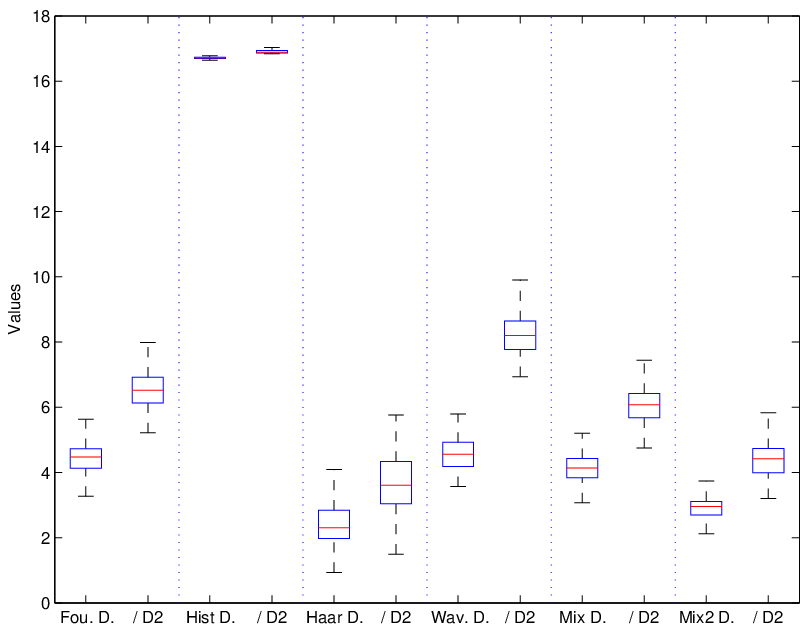
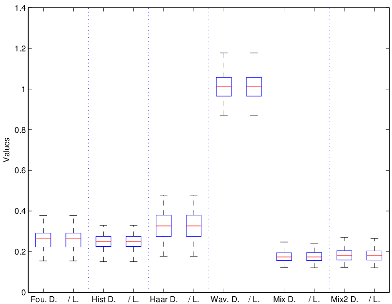
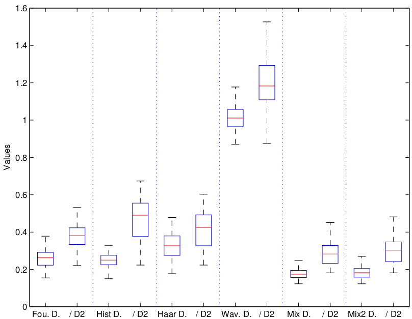
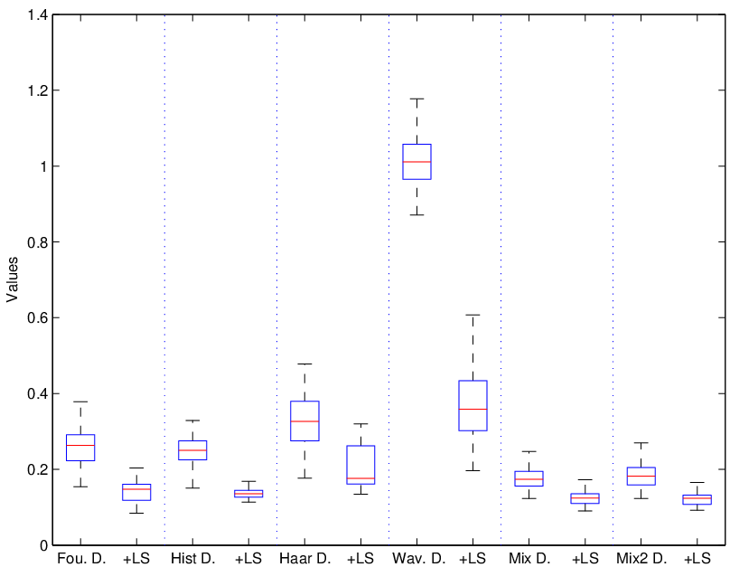
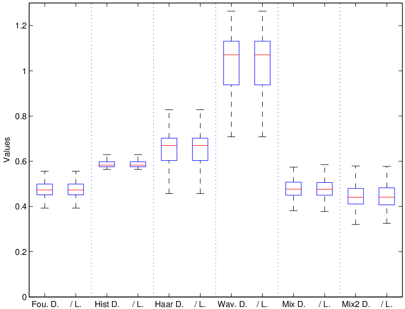
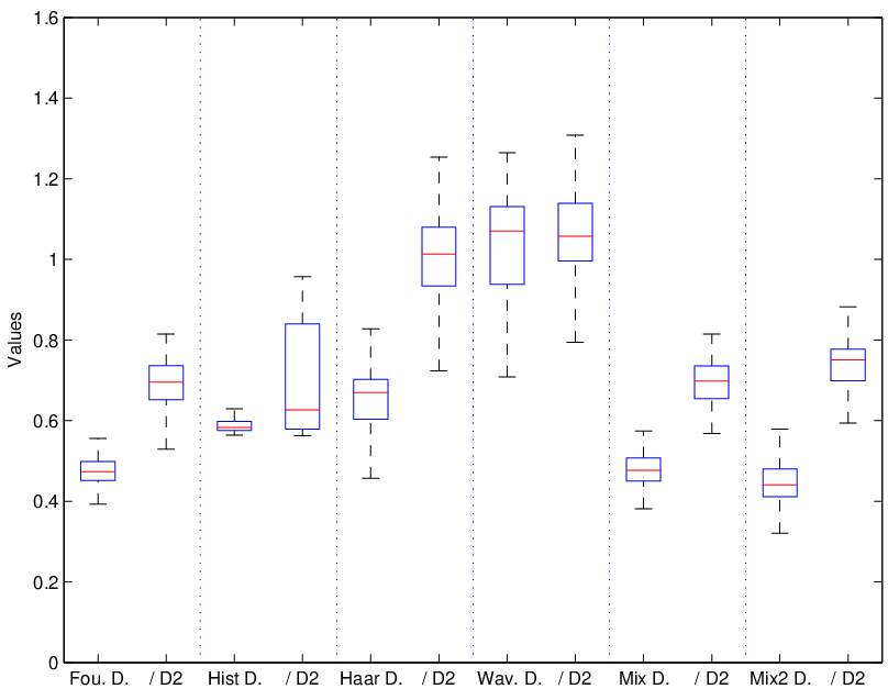
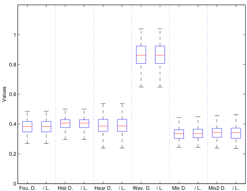
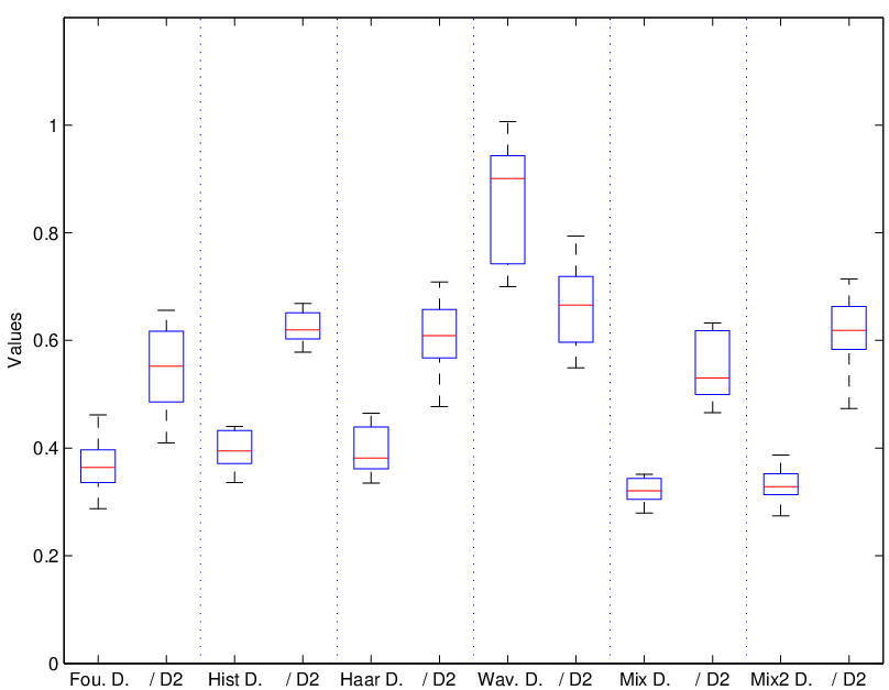
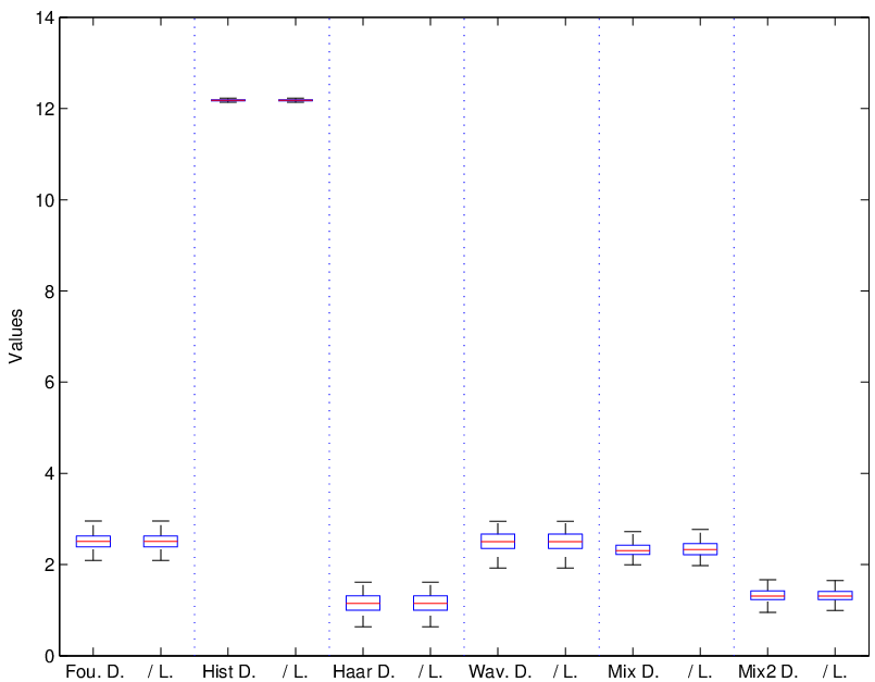
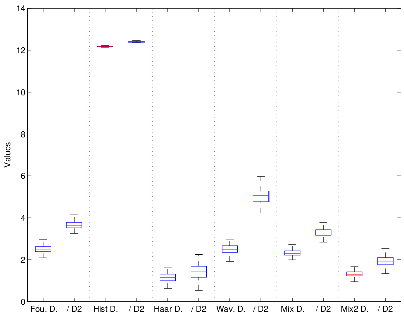
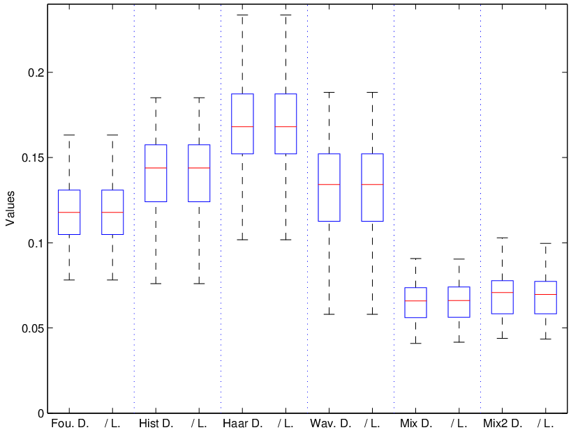
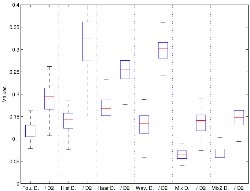
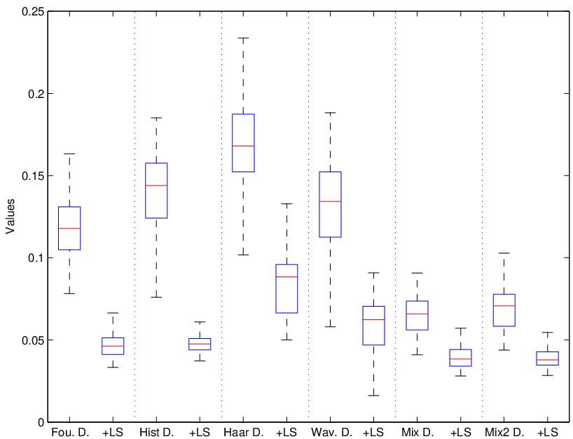
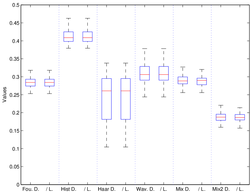
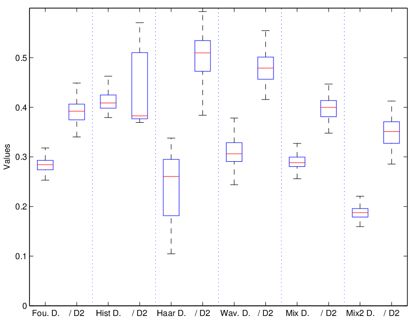
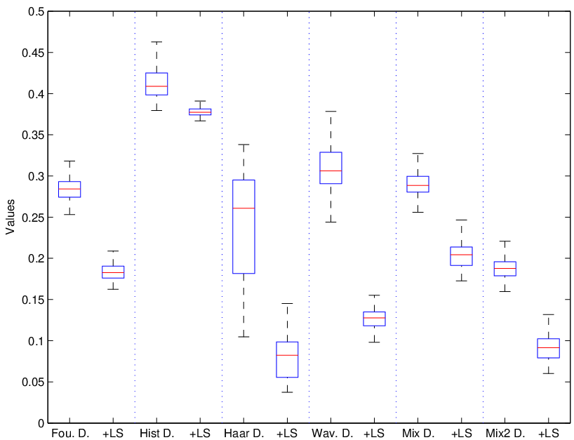
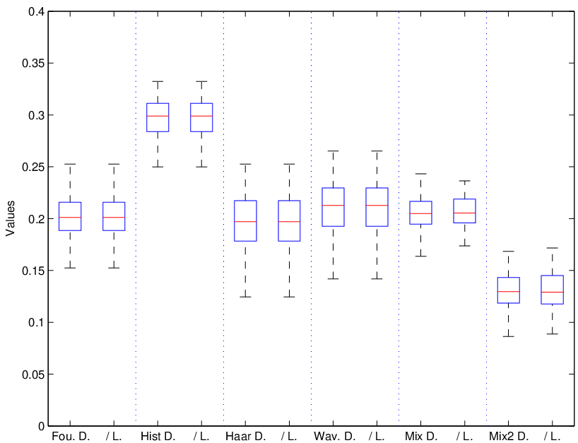
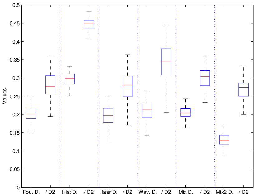
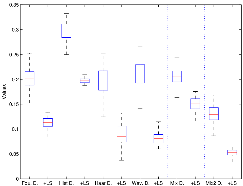
Boxplots of Figures 3 and 4 summarize our numerical experiments for n=500n=500 and n=2000n=2000 and 100100 repetitions of the procedures. The left column deals with the comparison between Dantzig and Lasso, the center column shows the effectiveness of our data driven constraint and the right column illustrates the improvement of the two-step method. As expected, Dantzig and Lasso estimators are strictly equivalent when the dictionary is orthonormal and very close otherwise. For both algorithms and most of the densities, the best solution appears to be the “Mix2” dictionary, except for the density f1f_{1} where the Haar wavelets are better for n=500n=500. This shows that the dictionary approach yields an improvement over the classical basis approach. One observes also that the “Mix” dictionary is better than the best of its constituent, namely the Fourier basis and the histogram family, which corroborates our theoretical results. The adaptive constraints are much tighter than their non adaptive counterparts and yield to much better numerical results. Our last series of experiments shows the significant improvement obtained with the least square step. As hinted by Candès and Tao [13], this can be explained by the bias common to ℓ1\ell_{1} methods which is partially removed by this final least square adjustment. Studying directly the performance of this estimator is a challenging task.

n=500n=500 n=1000n=1000 n=2000n=2000
f1f_{1} Refer to caption Refer to caption Refer to caption
f2f_{2} Refer to caption Refer to caption Refer to caption
f3f_{3} Refer to caption Refer to caption Refer to caption
f4f_{4} Refer to caption Refer to caption Refer to caption
Figure 2: The different densities and their “Mix2” estimates. Densities are plotted in blue while their estimates are plotted in black. The full line corresponds to the adaptive Dantzig studied in this paper while the dotted line corresponds to its least square variant.
Dantzig/Lasso Dantzig/Non adapt. Dantzig Dantzig/Dantzig+LS
f1f_{1} Refer to caption Refer to caption Refer to caption
f2f_{2} Refer to caption Refer to caption Refer to caption
f3f_{3} Refer to caption Refer to caption Refer to caption
f4f_{4} Refer to caption Refer to caption Refer to caption
Figure 3: Boxplots for n=500n=500. Left column: Dantzig and Lasso estimates. Center column: Dantzig estimates associated with adaptive and non-adaptive constraints. Right column: Our estimate and the two-step estimate.
Dantzig/Lasso Dantzig/Non adapt. Dantzig Dantzig/Dantzig+LS
f1f_{1} Refer to caption Refer to caption Refer to caption
f2f_{2} Refer to caption Refer to caption Refer to caption
f3f_{3} Refer to caption Refer to caption Refer to caption
f4f_{4} Refer to caption Refer to caption Refer to caption
Figure 4: Boxplots for n=2000n=2000. Left column: Dantzig and Lasso estimates. Center column: Dantzig estimates associated with adaptive and non-adaptive constraints. Right column: Our estimate and the two-step estimate.

6 Proofs

6.1 Proof of Theorem 1

To prove the first part of Theorem 1, we fix m∈{1,…,M}m\in\{1,\dots,M\} and we set for any i∈{1,…,n}i\in\{1,\dots,n\},

Wi=1n​(φm​(Xi)−β0,m)W_{i}=\frac{1}{n}\left(\varphi_{m}(X_{i})-\beta_{0,m}\right)

that satisfies almost surely

|Wi|≤2​‖φm‖∞n.|W_{i}|\leq\frac{2|\!|\varphi_{m}|\!|_{\infty}}{n}.

Then, we apply Bernstein’s Inequality (see [21] on pages 24 and 26) with the variables WiW_{i} and −Wi-W_{i}: for any u>0u>0,

ℙ⁡(|β^m−β0,m|≥2​σ0,m2​un+2​u​‖φm‖∞3​n)≤2​e−u.\mathbb{P}\left(|\hat{\beta}_{m}-\beta_{0,m}|\geq\sqrt{\frac{2\sigma_{0,m}^{2}u}{n}}+\frac{2u|\!|\varphi_{m}|\!|_{\infty}}{3n}\right)\leq 2e^{-u}. (18)

Now, let us decompose ^​σm2\hat{}\sigma^{2}_{m} in two terms:

^​σm2\displaystyle\hat{}\sigma^{2}_{m} =12​n​(n−1)​∑i≠j(φm​(Xi)−φm​(Xj))2\displaystyle=\frac{1}{2n(n-1)}\sum_{i\not=j}(\varphi_{m}(X_{i})-\varphi_{m}(X_{j}))^{2}
=12​n​∑i=1n(φm​(Xi)−β0,m)2+12​n​∑j=1n(φm​(Xj)−β0,m)2−2n⁡(n−1)∑i=2n∑j=1i−1(φm(Xi)−β0,m)(φm(Xj)−β0,m)\displaystyle\begin{split}&=\frac{1}{2n}\sum_{i=1}^{n}(\varphi_{m}(X_{i})-\beta_{0,m})^{2}+\frac{1}{2n}\sum_{j=1}^{n}(\varphi_{m}(X_{j})-\beta_{0,m})^{2}\\ &\mspace{40mu}-\frac{2}{n(n-1)}\sum_{i=2}^{n}\sum_{j=1}^{i-1}(\varphi_{m}(X_{i})-\beta_{0,m})(\varphi_{m}(X_{j})-\beta_{0,m})\end{split}
=sn−2n⁡(n−1)​un\displaystyle=s_{n}-\frac{2}{n(n-1)}u_{n}

with

sn=1n​∑i=1n(φm​(Xi)−β0,m)2​ and ​un=∑i=2n∑j=1i−1(φm​(Xi)−β0,m)​(φm​(Xj)−β0,m).s_{n}=\frac{1}{n}\sum_{i=1}^{n}(\varphi_{m}(X_{i})-\beta_{0,m})^{2}\mbox{ and }u_{n}=\sum_{i=2}^{n}\sum_{j=1}^{i-1}(\varphi_{m}(X_{i})-\beta_{0,m})(\varphi_{m}(X_{j})-\beta_{0,m}). (19)

Let us first focus on sns_{n} that is the main term of ^​σm2\hat{}\sigma^{2}_{m} by applying again Bernstein’s Inequality with

Yi=σ0,m2−(φm​(Xi)−β0,m)2nY_{i}=\frac{\sigma^{2}_{0,m}-(\varphi_{m}(X_{i})-\beta_{0,m})^{2}}{n}

which satisfies

Yi≤σ0,m2n.Y_{i}\leq\frac{\sigma^{2}_{0,m}}{n}.

One has that for any u>0u>0

ℙ⁡(σ0,m2≥sn+2​vm​u+σ0,m2​u3​n)≤e−u\mathbb{P}\left(\sigma^{2}_{0,m}\geq s_{n}+\sqrt{2v_{m}u}+\frac{\sigma^{2}_{0,m}u}{3n}\right)\leq e^{-u}

with

vm=1n​𝔼​([σ0,m2−(φm​(Xi)−β0,m)2]2).v_{m}=\frac{1}{n}\mathbb{E}\left(\left[\sigma^{2}_{0,m}-(\varphi_{m}(X_{i})-\beta_{0,m})^{2}\right]^{2}\right).

But we have

vm\displaystyle v_{m} =1n​(σ0,m4+𝔼⁡[(φm​(Xi)−β0,m)4]−2​σ0,m2​𝔼​[(φm​(Xi)−β0,m)2])\displaystyle=\frac{1}{n}\left(\sigma^{4}_{0,m}+\mathbb{E}\left[(\varphi_{m}(X_{i})-\beta_{0,m})^{4}\right]-2\sigma^{2}_{0,m}\mathbb{E}\left[(\varphi_{m}(X_{i})-\beta_{0,m})^{2}\right]\right)
=1n​(𝔼⁡[(φm​(Xi)−β0,m)4]−σ0,m4)\displaystyle=\frac{1}{n}\left(\mathbb{E}\left[(\varphi_{m}(X_{i})-\beta_{0,m})^{4}\right]-\sigma^{4}_{0,m}\right)
≤σ0,m2n​(‖φm‖∞+|β0,m|)2\displaystyle\leq\frac{\sigma^{2}_{0,m}}{n}\left(|\!|\varphi_{m}|\!|_{\infty}+|\beta_{0,m}|\right)^{2}
≤4​σ0,m2n​‖φm‖∞2.\displaystyle\leq\frac{4\sigma^{2}_{0,m}}{n}|\!|\varphi_{m}|\!|_{\infty}^{2}.

Finally, with for any u>0u>0

S⁡(u)=2​2​σ0,m​‖φm‖∞​un+σ0,m2​u3​n,S(u)=2\sqrt{2}\sigma_{0,m}|\!|\varphi_{m}|\!|_{\infty}\sqrt{\frac{u}{n}}+\frac{\sigma^{2}_{0,m}u}{3n},

we have

ℙ⁡(σ0,m2≥sn+S⁡(u))≤e−u.\mathbb{P}(\sigma^{2}_{0,m}\geq s_{n}+S(u))\leq e^{-u}. (20)

The term unu_{n} is a degenerate U-statistics that satisfies for any u>0u>0

ℙ⁡(|un|≥U⁡(u))≤6​e−u,\mathbb{P}(|u_{n}|\geq U(u))\leq 6e^{-u}, (21)

with for any u>0u>0

U⁡(u)=43​A​u2+(4​2+23)​B​u32+(2​D+23​F)​u+2​2​C​u,U(u)=\frac{4}{3}Au^{2}+\left(4\sqrt{2}+\frac{2}{3}\right)Bu^{\frac{3}{2}}+\left(2D+\frac{2}{3}F\right)u+2\sqrt{2}C\sqrt{u},

where AA, BB, CC, DD and FF are constants not depending on uu that satisfy

A\displaystyle A ≤4​‖φm‖∞2,\displaystyle\leq 4|\!|\varphi_{m}|\!|_{\infty}^{2},
B\displaystyle B ≤2​n−1​‖φm‖∞2,\displaystyle\leq 2\sqrt{n-1}|\!|\varphi_{m}|\!|_{\infty}^{2},
C\displaystyle C ≤n⁡(n−1)2​σ0,m2,\displaystyle\leq\sqrt{\frac{n(n-1)}{2}}\sigma^{2}_{0,m},
D\displaystyle D ≤n⁡(n−1)2​σ0,m2,\displaystyle\leq\sqrt{\frac{n(n-1)}{2}}\sigma^{2}_{0,m},
and
F\displaystyle F ≤2​2​‖φm‖∞2​(n−1)​log⁡(2​n)\displaystyle\leq 2\sqrt{2}|\!|\varphi_{m}|\!|_{\infty}^{2}\sqrt{(n-1)\log(2n)}

(see [27]). Then, we have for any u>0u>0,

2n⁡(n−1)​U​(u)\displaystyle\frac{2}{n(n-1)}U(u) ≤323​‖φm‖∞2n⁡(n−1)​u2+(16​2+83)​‖φm‖∞2n​n−1​u32\displaystyle\leq\frac{32}{3}\frac{|\!|\varphi_{m}|\!|_{\infty}^{2}}{n(n-1)}u^{2}+\left(16\sqrt{2}+\frac{8}{3}\right)\frac{|\!|\varphi_{m}|\!|_{\infty}^{2}}{n\sqrt{n-1}}u^{\frac{3}{2}}
+(2​2​σ0,m2n⁡(n−1)+8​23​log⁡(2​n)​‖φm‖∞2n​n−1)​u+4​σ0,m2n⁡(n−1)​u.\displaystyle\mspace{40mu}+\left(2\sqrt{2}\frac{\sigma^{2}_{0,m}}{\sqrt{n(n-1)}}+\frac{8\sqrt{2}}{3}\frac{\sqrt{\log(2n)}|\!|\varphi_{m}|\!|_{\infty}^{2}}{n\sqrt{n-1}}\right)u+\frac{4\sigma^{2}_{0,m}}{\sqrt{n(n-1)}}\sqrt{u}.

Now, we take uu that satisfies

u=o⁡(n)u=o(n) (22)

and

log⁡(2​n)≤2​u.\sqrt{\log(2n)}\leq\sqrt{2u}. (23)

Therefore, for any ε1>0\varepsilon_{1}>0, we have for nn large enough,

2n⁡(n−1)​U​(u)≤ε1​σ0,m2+(16​2+8)​‖φm‖∞2n​n−1​u32+323​‖φm‖∞2n⁡(n−1)​u2.\frac{2}{n(n-1)}U(u)\leq\varepsilon_{1}\sigma^{2}_{0,m}+\left(16\sqrt{2}+8\right)\frac{|\!|\varphi_{m}|\!|_{\infty}^{2}}{n\sqrt{n-1}}u^{\frac{3}{2}}+\frac{32}{3}\frac{|\!|\varphi_{m}|\!|_{\infty}^{2}}{n(n-1)}u^{2}.

So, for nn large enough,

2n⁡(n−1)​U​(u)≤ε1​σ0,m2+C1​‖φm‖∞2​(un)32,\frac{2}{n(n-1)}U(u)\leq\varepsilon_{1}\sigma^{2}_{0,m}+C_{1}|\!|\varphi_{m}|\!|_{\infty}^{2}\left(\frac{u}{n}\right)^{\frac{3}{2}}, (24)

where C1=16​2+19C_{1}=16\sqrt{2}+19. Using Inequalities (20) and (21), we obtain

ℙ⁡(σ0,m2≥^​σm2+S⁡(u)+2n⁡(n−1)​U​(u))\displaystyle\mathbb{P}\left(\sigma^{2}_{0,m}\geq\hat{}\sigma^{2}_{m}+S(u)+\frac{2}{n(n-1)}U(u)\right) =ℙ⁡(σ0,m2≥sn−2n⁡(n−1)​un+S⁡(u)+2n⁡(n−1)​U​(u))\displaystyle=\mathbb{P}\left(\sigma^{2}_{0,m}\geq s_{n}-\frac{2}{n(n-1)}u_{n}+S(u)+\frac{2}{n(n-1)}U(u)\right)
≤ℙ⁡(σ0,m2≥sn+S⁡(u))+ℙ⁡(un≥U⁡(u))\displaystyle\leq\mathbb{P}\left(\sigma^{2}_{0,m}\geq s_{n}+S(u)\right)+\mathbb{P}\left(u_{n}\geq U(u)\right)
≤7​e−u.\displaystyle\leq 7e^{-u}.

Now, using (24), for any 0<ε2<10<\varepsilon_{2}<1, we have for nn large enough,

^​σm2+S⁡(u)+2n⁡(n−1)​U​(u)\displaystyle\hat{}\sigma^{2}_{m}+S(u)+\frac{2}{n(n-1)}U(u) =^​σm2+2​2​σ0,m​‖φm‖∞​un+σ0,m2​u3​n+2n⁡(n−1)​U​(u)\displaystyle=\hat{}\sigma^{2}_{m}+2\sqrt{2}\sigma_{0,m}|\!|\varphi_{m}|\!|_{\infty}\sqrt{\frac{u}{n}}+\frac{\sigma_{0,m}^{2}u}{3n}+\frac{2}{n(n-1)}U(u)
≤^​σm2+2​2​σ0,m​‖φm‖∞​un+σ0,m2​u3​n+ε1​σ0,m2+C1​‖φm‖∞2​(un)32\displaystyle\leq\hat{}\sigma^{2}_{m}+2\sqrt{2}\sigma_{0,m}|\!|\varphi_{m}|\!|_{\infty}\sqrt{\frac{u}{n}}+\frac{\sigma_{0,m}^{2}u}{3n}+\varepsilon_{1}\sigma_{0,m}^{2}+C_{1}|\!|\varphi_{m}|\!|_{\infty}^{2}\left(\frac{u}{n}\right)^{\frac{3}{2}}
≤^​σm2+2​2​σ0,m​‖φm‖∞​un+ε2​σ0,m2+C1​‖φm‖∞2​(un)32.\displaystyle\leq\hat{}\sigma^{2}_{m}+2\sqrt{2}\sigma_{0,m}|\!|\varphi_{m}|\!|_{\infty}\sqrt{\frac{u}{n}}+\varepsilon_{2}\sigma^{2}_{0,m}+C_{1}|\!|\varphi_{m}|\!|_{\infty}^{2}\left(\frac{u}{n}\right)^{\frac{3}{2}}.

Therefore,

ℙ⁡((1−ε2)​σ0,m2≥^​σm2+2​2​σ0,m​‖φm‖∞​un+C1​‖φm‖∞2​(un)32)≤7​e−u.\mathbb{P}\left((1-\varepsilon_{2})\sigma^{2}_{0,m}\geq\hat{}\sigma^{2}_{m}+2\sqrt{2}\sigma_{0,m}|\!|\varphi_{m}|\!|_{\infty}\sqrt{\frac{u}{n}}+C_{1}|\!|\varphi_{m}|\!|_{\infty}^{2}\left(\frac{u}{n}\right)^{\frac{3}{2}}\right)\leq 7e^{-u}. (25)

Now, let us set

a=1−ε2,b=2​‖φm‖∞​un,c=^​σm2+C1​‖φm‖∞2​(un)32a=1-\varepsilon_{2},\quad b=\sqrt{2}|\!|\varphi_{m}|\!|_{\infty}\sqrt{\frac{u}{n}},\quad c=\hat{}\sigma^{2}_{m}+C_{1}|\!|\varphi_{m}|\!|_{\infty}^{2}\left(\frac{u}{n}\right)^{\frac{3}{2}}

and consider the polynomial

P⁡(x)=a​x2−2​b​x−c,P(x)=ax^{2}-2bx-c,

with roots b±b2+a​ca\frac{b\pm\sqrt{b^{2}+ac}}{a}. So, we have

P⁡(σ0,m)≥0\displaystyle P(\sigma_{0,m})\geq 0 ⟺σ0,m≥b+b2+a​ca\displaystyle\Longleftrightarrow\sigma_{0,m}\geq\frac{b+\sqrt{b^{2}+ac}}{a}
⟺σ0,m2≥ca+2​b2a2+2​b​b2+a​ca2.\displaystyle\Longleftrightarrow\sigma^{2}_{0,m}\geq\frac{c}{a}+\frac{2b^{2}}{a^{2}}+\frac{2b\sqrt{b^{2}+ac}}{a^{2}}.

It yields

ℙ⁡(σ0,m2≥ca+2​b2a2+2​b​b2+a​ca2)\displaystyle\mathbb{P}\left(\sigma^{2}_{0,m}\geq\frac{c}{a}+\frac{2b^{2}}{a^{2}}+\frac{2b\sqrt{b^{2}+ac}}{a^{2}}\right) ≤7​e−u,\displaystyle\leq 7e^{-u},
so,
ℙ⁡(σ0,m2≥ca+4​b2a2+2​b​ca​a)\displaystyle\mathbb{P}\left(\sigma^{2}_{0,m}\geq\frac{c}{a}+\frac{4b^{2}}{a^{2}}+\frac{2b\sqrt{c}}{a\sqrt{a}}\right) ≤7​e−u,\displaystyle\leq 7e^{-u},

which means that for any 0<ε3<10<\varepsilon_{3}<1, we have for nn large enough,

ℙ⁡(σ0,m2≥(1+ε3)​(^​σm2+C1​‖φm‖∞2​(un)32+8​‖φm‖∞2​un+2​2||φm||∞​un​^​σm2+C1​‖φm‖∞2​(un)32))\displaystyle\mathbb{P}\left(\sigma^{2}_{0,m}\geq(1+\varepsilon_{3})\left(\hat{}\sigma^{2}_{m}+C_{1}|\!|\varphi_{m}|\!|_{\infty}^{2}\left(\frac{u}{n}\right)^{\frac{3}{2}}+8|\!|\varphi_{m}|\!|_{\infty}^{2}\frac{u}{n}+2\sqrt{2}|\!|\varphi_{m}|\!|_{\infty}\sqrt{\frac{u}{n}}\sqrt{\hat{}\sigma^{2}_{m}+C_{1}|\!|\varphi_{m}|\!|_{\infty}^{2}\left(\frac{u}{n}\right)^{\frac{3}{2}}}\right)\right) ≤7​e−u.\displaystyle\leq 7e^{-u}.

Finally, we can claim that for any 0<ε4<10<\varepsilon_{4}<1, we have for nn large enough,

ℙ⁡(σ0,m2≥(1+ε4)​(^​σm2+8​‖φm‖∞2​un+2​‖φm‖∞​2​^​σm2​un))\displaystyle\mathbb{P}\left(\sigma^{2}_{0,m}\geq(1+\varepsilon_{4})\left(\hat{}\sigma^{2}_{m}+8|\!|\varphi_{m}|\!|_{\infty}^{2}\frac{u}{n}+2|\!|\varphi_{m}|\!|_{\infty}\sqrt{2\hat{}\sigma^{2}_{m}\frac{u}{n}}\right)\right) ≤7​e−u.\displaystyle\leq 7e^{-u}.

Now, we take u=γ​log⁡Mu=\gamma\log M. Under Assumptions of Theorem 1, Conditions (22) and (23) are satisfied. The previous concentration inequality means that

ℙ⁡(σ0,m2≥(1+ε4)​~​σm2)\displaystyle\mathbb{P}\left(\sigma^{2}_{0,m}\geq(1+\varepsilon_{4})\tilde{}\sigma^{2}_{m}\right) ≤7​M−γ.\displaystyle\leq 7M^{-\gamma}.

Now, using (18), we have for nn large enough,

ℙ⁡(|β0,m−β^m|≥ηγ,m)=ℙ⁡(|β0,m−β^m|≥2​~​σm2​γ​log⁡Mn+2​‖φm‖∞​γ​log⁡M3​n,σ0,m2<(1+ε4)​~​σm2)+ℙ⁡(|β0,m−β^m|≥ηγ,m,σ0,m2≥(1+ε4)​~​σm2)\displaystyle\begin{split}\mathbb{P}\left(|\beta_{0,m}-\hat{\beta}_{m}|\geq\eta_{\gamma,m}\right)&=\mathbb{P}\left(|\beta_{0,m}-\hat{\beta}_{m}|\geq\sqrt{\frac{2\tilde{}\sigma^{2}_{m}\gamma\log M}{n}}+\frac{2|\!|\varphi_{m}|\!|_{\infty}\gamma\log M}{3n},\ \sigma^{2}_{0,m}<(1+\varepsilon_{4})\tilde{}\sigma^{2}_{m}\right)\\ &\mspace{40mu}+\mathbb{P}\left(|\beta_{0,m}-\hat{\beta}_{m}|\geq\eta_{\gamma,m},\ \sigma^{2}_{0,m}\geq(1+\varepsilon_{4})\tilde{}\sigma^{2}_{m}\right)\end{split}
≤ℙ⁡(|β0,m−β^m|≥2​σ0,m2​γ​(1+ε4)−1​log⁡Mn+2​‖φm‖∞​γ​(1+ε4)−1​log⁡M3​n)+ℙ⁡(σ0,m2≥(1+ε4)​~​σ2)\displaystyle\begin{split}&\leq\mathbb{P}\left(|\beta_{0,m}-\hat{\beta}_{m}|\geq\sqrt{\frac{2\sigma^{2}_{0,m}\gamma(1+\varepsilon_{4})^{-1}\log M}{n}}+\frac{2|\!|\varphi_{m}|\!|_{\infty}\gamma(1+\varepsilon_{4})^{-1}\log M}{3n}\right)\\ &\mspace{40mu}+\mathbb{P}\left(\sigma^{2}_{0,m}\geq(1+\varepsilon_{4})\tilde{}\sigma^{2}\right)\end{split}
≤2​M−γ​(1+ε4)−1+7​M−γ.\displaystyle\leq 2M^{-\gamma(1+\varepsilon_{4})^{-1}}+7M^{-\gamma}.

Then, the first part of Theorem 1 is proved: for any ε>0\varepsilon>0,

ℙ⁡(|β0,m−β^m|≥ηγ,m)≤C⁡(ε,δ,γ)​M−γ1+ε,\mathbb{P}\left(|\beta_{0,m}-\hat{\beta}_{m}|\geq\eta_{\gamma,m}\right)\leq C(\varepsilon,\delta,\gamma)M^{-\frac{\gamma}{1+\varepsilon}},

where C⁡(ε,δ,γ)C(\varepsilon,\delta,\gamma) is a constant that depends on ε,\varepsilon, δ\delta and γ\gamma.

For the second part of the result, we apply again Bernstein’s Inequality with

Zi=(φm​(Xi)−β0,m)2−σ0,m2nZ_{i}=\frac{(\varphi_{m}(X_{i})-\beta_{0,m})^{2}-\sigma^{2}_{0,m}}{n}

which satisfies

Zi≤(φm​(Xi)−β0,m)2n≤4​‖φm‖∞2n.Z_{i}\leq\frac{(\varphi_{m}(X_{i})-\beta_{0,m})^{2}}{n}\leq\frac{4|\!|\varphi_{m}|\!|_{\infty}^{2}}{n}.

One has that for any u>0u>0

ℙ⁡(sn≥σ0,m2+2​vm​u+4​‖φm‖∞2​u3​n)≤e−u\mathbb{P}\left(s_{n}\geq\sigma^{2}_{0,m}+\sqrt{2v_{m}u}+\frac{4|\!|\varphi_{m}|\!|_{\infty}^{2}u}{3n}\right)\leq e^{-u}

with

vm=1n​𝔼​([σ0,m2−(φm​(Xi)−β0,m)2]2)≤4​σ0,m2n​‖φm‖∞2.v_{m}=\frac{1}{n}\mathbb{E}\left(\left[\sigma^{2}_{0,m}-(\varphi_{m}(X_{i})-\beta_{0,m})^{2}\right]^{2}\right)\leq\frac{4\sigma^{2}_{0,m}}{n}|\!|\varphi_{m}|\!|_{\infty}^{2}.

So, for any u>0u>0,

ℙ⁡(sn≥σ0,m2+2​2​σ0,m​‖φm‖∞​un+4​‖φm‖∞2​u3​n)≤e−u.\mathbb{P}\left(s_{n}\geq\sigma^{2}_{0,m}+2\sqrt{2}\sigma_{0,m}|\!|\varphi_{m}|\!|_{\infty}\sqrt{\frac{u}{n}}+\frac{4|\!|\varphi_{m}|\!|_{\infty}^{2}u}{3n}\right)\leq e^{-u}.

Now, for any ε5>0\varepsilon_{5}>0, for any u>0u>0,

ℙ⁡(sn≥(1+ε5)​σ0,m2+‖φm‖∞2​un​(43+2ε5))≤e−u.\mathbb{P}\left(s_{n}\geq(1+\varepsilon_{5})\sigma^{2}_{0,m}+\frac{|\!|\varphi_{m}|\!|_{\infty}^{2}u}{n}\left(\frac{4}{3}+\frac{2}{\varepsilon_{5}}\right)\right)\leq e^{-u}.

Using (21), with

S~​(u)=‖φm‖∞2​un​(43+2ε5),\tilde{S}(u)=\frac{|\!|\varphi_{m}|\!|_{\infty}^{2}u}{n}\left(\frac{4}{3}+\frac{2}{\varepsilon_{5}}\right),
ℙ⁡(^​σm2≥(1+ε5)​σ0,m2+S~​(u)+2n⁡(n−1)​U​(u))\displaystyle\mathbb{P}\left(\hat{}\sigma^{2}_{m}\geq(1+\varepsilon_{5})\sigma^{2}_{0,m}+\tilde{S}(u)+\frac{2}{n(n-1)}U(u)\right) =ℙ⁡(sn−2n⁡(n−1)​un≥(1+ε5)​σ0,m2+S~​(u)+2n⁡(n−1)​U​(u))\displaystyle=\mathbb{P}\left(s_{n}-\frac{2}{n(n-1)}u_{n}\geq(1+\varepsilon_{5})\sigma^{2}_{0,m}+\tilde{S}(u)+\frac{2}{n(n-1)}U(u)\right)
≤ℙ⁡(sn≥(1+ε5)​σ0,m2+S~​(u))+ℙ⁡(−un≥U⁡(u))\displaystyle\leq\mathbb{P}\left(s_{n}\geq(1+\varepsilon_{5})\sigma^{2}_{0,m}+\tilde{S}(u)\right)+\mathbb{P}\left(-u_{n}\geq U(u)\right)
≤e−u+6​e−u=7​e−u.\displaystyle\leq e^{-u}+6e^{-u}=7e^{-u}.

Using (24),

ℙ⁡(^​σm2≥(1+ε1+ε5)​σ0,m2+S~​(u)+C1​‖φm‖∞2​(un)32)\displaystyle\mathbb{P}\left(\hat{}\sigma^{2}_{m}\geq(1+\varepsilon_{1}+\varepsilon_{5})\sigma^{2}_{0,m}+\tilde{S}(u)+C_{1}|\!|\varphi_{m}|\!|_{\infty}^{2}\left(\frac{u}{n}\right)^{\frac{3}{2}}\right) ≤7​e−u.\displaystyle\leq 7e^{-u}.

Since

ηγ,m=2​~​σm2​γ​log⁡Mn+2​‖φm‖∞​γ​log⁡M3​n,\eta_{\gamma,m}=\sqrt{\frac{2\tilde{}\sigma^{2}_{m}\gamma\log M}{n}}+\frac{2|\!|\varphi_{m}|\!|_{\infty}\gamma\log M}{3n},

with

~​σm2=^​σm2+2​‖φm‖∞​2​^​σm2​γ​log⁡Mn+8​‖φm‖∞2​γ​log⁡Mn,\tilde{}\sigma^{2}_{m}=\hat{}\sigma^{2}_{m}+2|\!|\varphi_{m}|\!|_{\infty}\sqrt{\frac{2\hat{}\sigma^{2}_{m}\gamma\log M}{n}}+\frac{8|\!|\varphi_{m}|\!|_{\infty}^{2}\gamma\log M}{n},

we have for any ε6>0\varepsilon_{6}>0,

ηγ,m2\displaystyle\eta_{\gamma,m}^{2} ≤(1+ε6)​(2​~​σm2​γ​log⁡Mn)+(1+ε6−1)​(4​‖φm‖∞2​(γ​log⁡M)29​n2)\displaystyle\leq(1+\varepsilon_{6})\left(\frac{2\tilde{}\sigma^{2}_{m}\gamma\log M}{n}\right)+(1+\varepsilon_{6}^{-1})\left(\frac{4|\!|\varphi_{m}|\!|_{\infty}^{2}(\gamma\log M)^{2}}{9n^{2}}\right)
≤(1+ε6)​(2​γ​log⁡Mn)​(^​σm2+2​‖φm‖∞​2​^​σm2​γ​log⁡Mn+8​‖φm‖∞2​γ​log⁡Mn)+49​(1+ε6−1)​(‖φm‖∞​γ​log⁡Mn)2\displaystyle\begin{split}&\leq(1+\varepsilon_{6})\left(\frac{2\gamma\log M}{n}\right)\left(\hat{}\sigma^{2}_{m}+2|\!|\varphi_{m}|\!|_{\infty}\sqrt{\frac{2\hat{}\sigma^{2}_{m}\gamma\log M}{n}}+\frac{8|\!|\varphi_{m}|\!|_{\infty}^{2}\gamma\log M}{n}\right)\\ &\mspace{40mu}+\frac{4}{9}(1+\varepsilon_{6}^{-1})\left(\frac{|\!|\varphi_{m}|\!|_{\infty}\gamma\log M}{n}\right)^{2}\end{split}
≤(1+ε6)2​^​σm2​(2​γ​log⁡Mn)+4​ε6−1​(1+ε6)​(‖φm‖∞​γ​log⁡Mn)2+16​(1+ε6)​(‖φm‖∞​γ​log⁡Mn)2+4​(1+ε6−1)9​(‖φm‖∞​γ​log⁡Mn)2.\displaystyle\begin{split}&\leq(1+\varepsilon_{6})^{2}\hat{}\sigma^{2}_{m}\left(\frac{2\gamma\log M}{n}\right)+4\varepsilon_{6}^{-1}(1+\varepsilon_{6})\left(\frac{|\!|\varphi_{m}|\!|_{\infty}\gamma\log M}{n}\right)^{2}\\ &\mspace{40mu}+16(1+\varepsilon_{6})\left(\frac{|\!|\varphi_{m}|\!|_{\infty}\gamma\log M}{n}\right)^{2}+\frac{4(1+\varepsilon_{6}^{-1})}{9}\left(\frac{|\!|\varphi_{m}|\!|_{\infty}\gamma\log M}{n}\right)^{2}.\end{split}

Finally, with u=γ​log⁡Mu=\gamma\log M, with probability larger than 1−7​M−γ1-7M^{-\gamma},

^​σm2<(1+ε1+ε5)​σ0,m2+S~​(γ​log⁡M)+C1​‖φm‖∞2​(γ​log⁡Mn)32,\hat{}\sigma^{2}_{m}<(1+\varepsilon_{1}+\varepsilon_{5})\sigma^{2}_{0,m}+\tilde{S}(\gamma\log M)+C_{1}|\!|\varphi_{m}|\!|_{\infty}^{2}\left(\frac{\gamma\log M}{n}\right)^{\frac{3}{2}},

and

ηγ,m2<(1+ε6)2​(1+ε5+ε1)​σ0,m2​(2​γ​log⁡Mn)+(1+ε6)2​(γ​log⁡Mn)2​‖φm‖∞2​(83+4ε5)+2​C1​(1+ε6)2​‖φm‖∞2​(γ​log⁡Mn)52+‖φm‖∞2​(γ​log⁡Mn)2​(4​ε6−1​(1+ε6)+16​(1+ε6)+4​(1+ε6−1)9).\displaystyle\begin{split}\eta_{\gamma,m}^{2}&<(1+\varepsilon_{6})^{2}(1+\varepsilon_{5}+\varepsilon_{1})\sigma^{2}_{0,m}\left(\frac{2\gamma\log M}{n}\right)+(1+\varepsilon_{6})^{2}\left(\frac{\gamma\log M}{n}\right)^{2}|\!|\varphi_{m}|\!|_{\infty}^{2}\left(\frac{8}{3}+\frac{4}{\varepsilon_{5}}\right)\\ &\mspace{40mu}+2C_{1}(1+\varepsilon_{6})^{2}|\!|\varphi_{m}|\!|_{\infty}^{2}\left(\frac{\gamma\log M}{n}\right)^{\frac{5}{2}}+|\!|\varphi_{m}|\!|_{\infty}^{2}\left(\frac{\gamma\log M}{n}\right)^{2}\left(4\varepsilon_{6}^{-1}(1+\varepsilon_{6})+16(1+\varepsilon_{6})+\frac{4(1+\varepsilon_{6}^{-1})}{9}\right).\end{split}

Finally, with ε6=1\varepsilon_{6}=1, ε1=ε5=12\varepsilon_{1}=\varepsilon_{5}=\frac{1}{2}, for nn large enough,

ℙ⁡(ηγ,m≥4​σ0,m​γ​log⁡Mn+10​‖φm‖∞​γ​log⁡Mn)≤7​M−γ.\mathbb{P}\left(\eta_{\gamma,m}\geq 4\sigma_{0,m}\sqrt{\frac{\gamma\log M}{n}}+\frac{10|\!|\varphi_{m}|\!|_{\infty}\gamma\log M}{n}\right)\leq 7M^{-\gamma}.

Note that 32/3+32+8+32+8/9=9.1409\sqrt{32/3+32+8+32+8/9}=9.1409.

For the last part, starting from (25) with u=γ​log⁡Mu=\gamma\log M and ε2=17\varepsilon_{2}=\frac{1}{7}, we have for nn large enough and with probability larger than 1−7​M−γ1-7M^{-\gamma},

67​σ0,m2\displaystyle\frac{6}{7}\sigma^{2}_{0,m} ≤^​σm2+2​2​σ0,m​‖φm‖∞​γ​log⁡Mn+C1​‖φm‖∞2​(γ​log⁡Mn)32\displaystyle\leq\hat{}\sigma^{2}_{m}+2\sqrt{2}\sigma_{0,m}|\!|\varphi_{m}|\!|_{\infty}\sqrt{\frac{\gamma\log M}{n}}+C_{1}|\!|\varphi_{m}|\!|_{\infty}^{2}\left(\frac{\gamma\log M}{n}\right)^{\frac{3}{2}}
≤^​σm2+27​σ0,m2+7​‖φm‖∞2​γ​log⁡Mn+C1​‖φm‖∞2​(γ​log⁡Mn)32.\displaystyle\leq\hat{}\sigma^{2}_{m}+\frac{2}{7}\sigma^{2}_{0,m}+7|\!|\varphi_{m}|\!|_{\infty}^{2}\frac{\gamma\log M}{n}+C_{1}|\!|\varphi_{m}|\!|_{\infty}^{2}\left(\frac{\gamma\log M}{n}\right)^{\frac{3}{2}}.

So, for nn large enough,

47​σ0,m2≤^​σm2+8​‖φm‖∞2​γ​log⁡Mn≤~​σm2\frac{4}{7}\sigma^{2}_{0,m}\leq\hat{}\sigma^{2}_{m}+8|\!|\varphi_{m}|\!|_{\infty}^{2}\frac{\gamma\log M}{n}\leq\tilde{}\sigma^{2}_{m}

and

ηγ,m>σ0,m​8​γ​log⁡M7​n+2​‖φm‖∞​γ​log⁡M3​n.\eta_{\gamma,m}>\sigma_{0,m}\sqrt{\frac{8\gamma\log M}{7n}}+\frac{2|\!|\varphi_{m}|\!|_{\infty}\gamma\log M}{3n}.

6.2 Proof of Theorem 2

Let λ=(λm)m=1,…,M\lambda=(\lambda_{m})_{m=1,\ldots,M} and set Δ=λ−λ^D\Delta=\lambda-\hat{\lambda}^{D}. We have

‖fλ−f0‖22=||f^D−f0||22+‖fλ−f^D‖22+2​∫(f^D​(x)−f0​(x))​(fλ​(x)−f^D​(x))​𝑑x.|\!|f_{\lambda}-f_{0}|\!|_{2}^{2}=|\!|\hat{f}^{D}-f_{0}|\!|_{2}^{2}+|\!|f_{\lambda}-\hat{f}^{D}|\!|_{2}^{2}+2\int(\hat{f}^{D}(x)-f_{0}(x))(f_{\lambda}(x)-\hat{f}^{D}(x))dx. (26)

We have ‖fλ−f^D‖22=‖fΔ‖22|\!|f_{\lambda}-\hat{f}^{D}|\!|_{2}^{2}=|\!|f_{\Delta}|\!|_{2}^{2}. Moreover, with probability at least 1−C1​(ε,δ,γ)​M1−γ1+ε1-C_{1}(\varepsilon,\delta,\gamma)M^{1-\frac{\gamma}{1+\varepsilon}}, we have

|∫(f^D​(x)−f0​(x))​(fλ​(x)−f^D​(x))​𝑑x|=\displaystyle\left|\int(\hat{f}^{D}(x)-f_{0}(x))(f_{\lambda}(x)-\hat{f}^{D}(x))dx\right|= |∑m=1M(λm−λ^mD)​[(G​λ^D)m−β0,m]|\displaystyle\left|\sum_{m=1}^{M}(\lambda_{m}-\hat{\lambda}_{m}^{D})\left[(G\hat{\lambda}^{D})_{m}-\beta_{0,m}\right]\right| (27)
≤\displaystyle\leq ‖Δ‖ℓ1​2​‖ηγ‖ℓ∞,\displaystyle|\!|\Delta|\!|_{\ell_{1}}2|\!|\eta_{\gamma}|\!|_{\ell_{\infty}},

where the last line is a consequence of the definition of the Dantzig estimator and of Theorem 1. Then, we have

‖f^D−f0‖22≤||fλ−f0||22+4​‖ηγ‖ℓ∞​‖Δ‖ℓ1−|​|fΔ||22.|\!|\hat{f}^{D}-f_{0}|\!|_{2}^{2}\leq|\!|f_{\lambda}-f_{0}|\!|_{2}^{2}+4|\!|\eta_{\gamma}|\!|_{\ell_{\infty}}|\!|\Delta|\!|_{\ell_{1}}-|\!|f_{\Delta}|\!|_{2}^{2}.

We use then the following Lemma:

Lemma 1.

Let J⊂{1,…,M}J\subset\{1,\ldots,M\}. For any λ∈ℝM\lambda\in\mathbb{R}^{M}

‖ΔJC‖ℓ1≤||ΔJ||ℓ1+2​‖λJC‖ℓ1+(‖^​λD‖ℓ1−||λ||ℓ1)+,|\!|\Delta_{J^{C}}|\!|_{\ell_{1}}\leq|\!|\Delta_{J}|\!|_{\ell_{1}}+2|\!|\lambda_{J^{C}}|\!|_{\ell_{1}}+\left(|\!|\hat{}\lambda^{D}|\!|_{\ell_{1}}-|\!|\lambda|\!|_{\ell_{1}}\right)_{+},

where Δ=λ^D−λ\Delta=\hat{\lambda}^{D}-\lambda.

Proof.[Proof of Lemma 1] This lemma is based on the fact that

‖^​λD‖ℓ1≤‖λ‖ℓ1+(‖^​λD‖ℓ1−||λ||ℓ1)+,|\!|\hat{}\lambda^{D}|\!|_{\ell_{1}}\leq|\!|\lambda|\!|_{\ell_{1}}+\left(|\!|\hat{}\lambda^{D}|\!|_{\ell_{1}}-|\!|\lambda|\!|_{\ell_{1}}\right)_{+},

which implies that

‖ΔJ+λJ‖ℓ1+‖ΔJC+λJC‖ℓ1≤||λJ||ℓ1+‖λJC‖ℓ1+(‖^​λD‖ℓ1−||λ||ℓ1)+,|\!|\Delta_{J}+\lambda_{J}|\!|_{\ell_{1}}+|\!|\Delta_{J^{C}}+\lambda_{J^{C}}|\!|_{\ell_{1}}\leq|\!|\lambda_{J}|\!|_{\ell_{1}}+|\!|\lambda_{J^{C}}|\!|_{\ell_{1}}+\left(|\!|\hat{}\lambda^{D}|\!|_{\ell_{1}}-|\!|\lambda|\!|_{\ell_{1}}\right)_{+},

and thus

‖λJ‖ℓ1−||ΔJ||ℓ1+‖ΔJC‖ℓ1−|​|λJC||ℓ1≤||λJ||ℓ1+‖λJC‖ℓ1+(‖^​λD‖ℓ1−||λ||ℓ1)+.|\!|\lambda_{J}|\!|_{\ell_{1}}-|\!|\Delta_{J}|\!|_{\ell_{1}}+|\!|\Delta_{J^{C}}|\!|_{\ell_{1}}-|\!|\lambda_{J^{C}}|\!|_{\ell_{1}}\leq|\!|\lambda_{J}|\!|_{\ell_{1}}+|\!|\lambda_{J^{C}}|\!|_{\ell_{1}}+\left(|\!|\hat{}\lambda^{D}|\!|_{\ell_{1}}-|\!|\lambda|\!|_{\ell_{1}}\right)_{+}.

■\blacksquare

Note that if λ\lambda satisfies the Dantzig condition then by definition of ^​λD\hat{}\lambda^{D}: (‖^​λD‖ℓ1−‖λ‖ℓ1)+=0\left(|\!|\hat{}\lambda^{D}|\!|_{\ell_{1}}-|\!|\lambda|\!|_{\ell_{1}}\right)_{+}=0. Using the previous lemma, we have:

(‖ΔJ0C‖ℓ1−||ΔJ0||ℓ1)+≤2​‖λJ0C‖ℓ1+(‖^​λD‖ℓ1−||λ||ℓ1)+.\left(|\!|\Delta_{J_{0}^{C}}|\!|_{\ell_{1}}-|\!|\Delta_{J_{0}}|\!|_{\ell_{1}}\right)_{+}\leq 2|\!|\lambda_{J_{0}^{C}}|\!|_{\ell_{1}}+\left(|\!|\hat{}\lambda^{D}|\!|_{\ell_{1}}-|\!|\lambda|\!|_{\ell_{1}}\right)_{+}.

Using now Λ⁡(λ,J0c)=‖λJ0C‖ℓ1+(‖^​λD‖ℓ1−‖λ‖ℓ1)+2\Lambda(\lambda,J_{0}^{c})=|\!|\lambda_{J_{0}^{C}}|\!|_{\ell_{1}}+\frac{\left(|\!|\hat{}\lambda^{D}|\!|_{\ell_{1}}-|\!|\lambda|\!|_{\ell_{1}}\right)_{+}}{2}, so that Λ⁡(λ,J0c)=‖λJ0C‖ℓ1\Lambda(\lambda,J_{0}^{c})=|\!|\lambda_{J_{0}^{C}}|\!|_{\ell_{1}} as soon as λ\lambda satisfies the Dantzig condition, we obtain

‖fΔ‖2\displaystyle|\!|f_{\Delta}|\!|_{2} ≥κJ0​‖ΔJ0‖ℓ2−μJ0​(‖ΔJ0C‖ℓ1−‖ΔJ0‖ℓ1)+\displaystyle\geq\kappa_{J_{0}}|\!|\Delta_{J_{0}}|\!|_{\ell_{2}}-\mu_{J_{0}}\left(|\!|\Delta_{J_{0}^{C}}|\!|_{\ell_{1}}-|\!|\Delta_{J_{0}}|\!|_{\ell_{1}}\right)_{+}
≥κJ0​‖ΔJ0‖ℓ2−2​μJ0​Λ​(λ,J0c)\displaystyle\geq\kappa_{J_{0}}|\!|\Delta_{J_{0}}|\!|_{\ell_{2}}-2\mu_{J_{0}}\Lambda(\lambda,J_{0}^{c})

and thus

‖ΔJ0‖ℓ2≤1κJ0​‖fΔ‖2+2​μJ0κJ0​Λ​(λ,J0c).\displaystyle|\!|\Delta_{J_{0}}|\!|_{\ell_{2}}\leq\frac{1}{\kappa_{J_{0}}}|\!|f_{\Delta}|\!|_{2}+2\frac{\mu_{J_{0}}}{\kappa_{J_{0}}}\Lambda(\lambda,J_{0}^{c}).

We deduce thus

‖Δ‖ℓ1\displaystyle|\!|\Delta|\!|_{\ell_{1}} ≤2​‖ΔJ0‖ℓ1+2​Λ​(λ,J0c)\displaystyle\leq 2|\!|\Delta_{J_{0}}|\!|_{\ell_{1}}+2\Lambda(\lambda,J_{0}^{c})
≤2​|J0|​‖ΔJ0‖ℓ2+2​‖λJ0C‖ℓ1~\displaystyle\leq 2\sqrt{|J_{0}|}|\!|\Delta_{J_{0}}|\!|_{\ell_{2}}+2\widetilde{|\!|\lambda_{J_{0}^{C}}|\!|_{\ell_{1}}}
≤2​|J0|κJ0​‖fΔ‖2+2​Λ​(λ,J0c)​(1+2​μJ0​|J0|κJ0)\displaystyle\leq\frac{2\sqrt{|J_{0}|}}{\kappa_{J_{0}}}|\!|f_{\Delta}|\!|_{2}+2\Lambda(\lambda,J_{0}^{c})\left(1+\frac{2\mu_{J_{0}}\sqrt{|J_{0}|}}{\kappa_{J_{0}}}\right)

and then since

4​‖ηγ‖ℓ∞​2​|J0|κJ0​‖fΔ‖2≤16​|J0|​‖ηγ‖ℓ∞2κJ02+||fΔ||224|\!|\eta_{\gamma}|\!|_{\ell_{\infty}}\frac{2\sqrt{|J_{0}|}}{\kappa_{J_{0}}}|\!|f_{\Delta}|\!|_{2}\leq\frac{16|J_{0}||\!|\eta_{\gamma}|\!|_{\ell_{\infty}}^{2}}{\kappa_{J_{0}}^{2}}+|\!|f_{\Delta}|\!|_{2}^{2}

we have

4||ηγ||ℓ∞​‖Δ‖ℓ1−‖fΔ‖22\displaystyle 4|\!|\eta_{\gamma}|\!|_{\ell_{\infty}}|\!|\Delta|\!|_{\ell_{1}}-|\!|f_{\Delta}|\!|_{2}^{2} ≤16​|J0|​‖ηγ‖ℓ∞2κJ02+8​‖ηγ‖ℓ∞​Λ​(λ,J0c)​(1+2​μJ0​|J0|κJ0)\displaystyle\leq\frac{16|J_{0}||\!|\eta_{\gamma}|\!|_{\ell_{\infty}}^{2}}{\kappa_{J_{0}}^{2}}+8|\!|\eta_{\gamma}|\!|_{\ell_{\infty}}\Lambda(\lambda,J_{0}^{c})\left(1+\frac{2\mu_{J_{0}}\sqrt{|J_{0}|}}{\kappa_{J_{0}}}\right)
≤16​|J0|​(1β+1κJ02)​‖ηγ‖ℓ∞2+β​Λ​(λ,J0c)2|J0|​(1+2​μJ0​|J0|κJ0)2,\displaystyle\leq 16|J_{0}|\left(\frac{1}{\beta}+\frac{1}{\kappa_{J_{0}}^{2}}\right)|\!|\eta_{\gamma}|\!|_{\ell_{\infty}}^{2}+\beta\frac{\Lambda(\lambda,J_{0}^{c})^{2}}{|J_{0}|}\left(1+\frac{2\mu_{J_{0}}\sqrt{|J_{0}|}}{\kappa_{J_{0}}}\right)^{2},

which is the result of the theorem.

6.3 Consequences of Assumptions 1 and 2

To prove Proposition 1, we establish Lemmas 2 and 3. In the sequel, we consider two integers ss and ll such that 1≤s≤M/21\leq s\leq M/2, l≥sl\geq s and s+l≤Ms+l\leq M. We first recall Assumptions 1 and 2. Assumption 1 is stated in a more general form, which allows to unify the statement of the subsequent results.

  • •

    Assumption 1

    ϕmin​(s+l)>θl,s+l.\phi_{\min}(s+l)>\theta_{l,s+l}.
  • •

    Assumption 2

    l​ϕmin​(s+l)>s​ϕmax​(l).l\phi_{\min}(s+l)>s\phi_{\max}(l).

In the sequel, we assume that Assumptions 1 and 2 are both true.

Lemma 2.

Let J0⊂{1,…,M}J_{0}\subset\{1,\ldots,M\} with cardinality |J0|=s|J_{0}|=s and Δ∈ℝM\Delta\in\mathbb{R}^{M}. We denote by J1J_{1} the subset of {1,…,M}\{1,\ldots,M\} corresponding to the ll largest coordinates of Δ\Delta (in absolute value) outside J0J_{0} and we set J01=J0∪J1J_{01}=J_{0}\cup J_{1}. We denote by PJ01P_{J_{01}} the projector on the linear space spanned by (φm)m∈J01(\varphi_{m})_{m\in J_{01}}. We have:

‖PJ01​fΔ‖2≥ϕmin​(s+l)​‖ΔJ01‖ℓ2−min⁡(μ1,μ2)||ΔJ0C||ℓ1,\displaystyle|\!|P_{J_{01}}f_{\Delta}|\!|_{2}\geq\sqrt{\phi_{\min}(s+l)}|\!|\Delta_{J_{01}}|\!|_{\ell_{2}}-\min\left(\mu_{1},\mu_{2}\right)|\!|\Delta_{J_{0}^{C}}|\!|_{\ell_{1}},

with

μ1=θl,s+ll​ϕmin​(s+l)andμ2=ϕmax​(l)l.\mu_{1}=\frac{\theta_{l,s+l}}{\sqrt{l\phi_{\min}(s+l)}}\quad\mbox{and}\quad\mu_{2}=\sqrt{\frac{\phi_{\max}(l)}{l}}.

Proof. For k>1k>1, we denote by JkJ_{k} the indices corresponding to the coordinates of Δ\Delta outside J0J_{0} whose absolute values are between the ((k−1)×l+1)((k-1)\times l+1)–th and the (k×l)(k\times l)–th largest ones (in absolute value). Note that this definition is consistent with the definition of J1J_{1}. Using this notation, we have

‖PJ01​fΔ‖2\displaystyle|\!|P_{J_{01}}f_{\Delta}|\!|_{2} ≥‖PJ01​fΔJ01‖2−‖∑k≥2PJ01​fΔJk‖2\displaystyle\geq|\!|P_{J_{01}}f_{\Delta_{J_{01}}}|\!|_{2}-|\!|\sum_{k\geq 2}P_{J_{01}}f_{\Delta_{J_{k}}}|\!|_{2}
≥‖fΔJ01‖2−∑k≥2‖PJ01​fΔJk‖2.\displaystyle\geq|\!|f_{\Delta_{J_{01}}}|\!|_{2}-\sum_{k\geq 2}|\!|P_{J_{01}}f_{\Delta_{J_{k}}}|\!|_{2}.

Since J01J_{01} has s+ls+l elements, we have

‖fΔJ01‖2≥ϕmin​(s+l)​‖ΔJ01‖ℓ2.|\!|f_{\Delta_{J_{01}}}|\!|_{2}\geq\sqrt{\phi_{\min}(s+l)}|\!|\Delta_{J_{01}}|\!|_{\ell_{2}}.

Note that PJ01​fΔJk=fCJ01P_{J_{01}}f_{\Delta_{J_{k}}}=f_{C_{J_{01}}} for some vector C∈ℝMC\in\mathbb{R}^{M}. Since,

⟨PJ01​fΔJk−fΔJk,PJ01​fΔJk⟩=0,\langle P_{J_{01}}f_{\Delta_{J_{k}}}-f_{\Delta_{J_{k}}},P_{J_{01}}f_{\Delta_{J_{k}}}\rangle=0,

one obtains that

‖PJ01​fΔJk‖22\displaystyle|\!|P_{J_{01}}f_{\Delta_{J_{k}}}|\!|_{2}^{2} =⟨fΔJk,fCJ01⟩\displaystyle=\langle f_{\Delta_{J_{k}}},f_{C_{J_{01}}}\rangle
and thus
‖PJ01​fΔJk‖22\displaystyle|\!|P_{J_{01}}f_{\Delta_{J_{k}}}|\!|_{2}^{2} ≤θl,s+l​‖ΔJk‖ℓ2​‖CJ01‖ℓ2≤θl,s+l||ΔJk||ℓ2​‖fCJ01‖2ϕmin​(s+l)\displaystyle\leq\theta_{l,s+l}|\!|\Delta_{J_{k}}|\!|_{\ell_{2}}|\!|C_{J_{01}}|\!|_{\ell_{2}}\leq\theta_{l,s+l}|\!|\Delta_{J_{k}}|\!|_{\ell_{2}}\frac{|\!|f_{C_{J_{01}}}|\!|_{2}}{\sqrt{\phi_{\min}(s+l)}}
≤θl,s+lϕmin​(s+l)​‖ΔJk‖ℓ2​‖PJ01​fΔJk‖2.\displaystyle\leq\frac{\theta_{l,s+l}}{\sqrt{\phi_{\min}(s+l)}}|\!|\Delta_{J_{k}}|\!|_{\ell_{2}}|\!|P_{J_{01}}f_{\Delta_{J_{k}}}|\!|_{2}.
This implies that
‖PJ01​fΔJk‖2\displaystyle|\!|P_{J_{01}}f_{\Delta_{J_{k}}}|\!|_{2} ≤θl,s+lϕmin​(s+l)​‖ΔJk‖ℓ2=μ1​l​‖ΔJk‖ℓ2.\displaystyle\leq\frac{\theta_{l,s+l}}{\sqrt{\phi_{\min}(s+l)}}|\!|\Delta_{J_{k}}|\!|_{\ell_{2}}=\mu_{1}\sqrt{l}|\!|\Delta_{J_{k}}|\!|_{\ell_{2}}.

Moreover, using that JkJ_{k} has less than ll elements, we obtain that

‖PJ01​fΔJk‖2≤‖fΔJk‖2≤ϕmax​(l)​‖ΔJk‖ℓ2=μ2​l||ΔJk||ℓ2.|\!|P_{J_{01}}f_{\Delta_{J_{k}}}|\!|_{2}\leq|\!|f_{\Delta_{J_{k}}}|\!|_{2}\leq\sqrt{\phi_{\max}(l)}|\!|\Delta_{J_{k}}|\!|_{\ell_{2}}=\mu_{2}\sqrt{l}|\!|\Delta_{J_{k}}|\!|_{\ell_{2}}.

Now using that ‖ΔJk+1‖ℓ2≤‖ΔJk‖ℓ1/l|\!|\Delta_{J_{k+1}}|\!|_{\ell_{2}}\leq|\!|\Delta_{J_{k}}|\!|_{\ell_{1}}/\sqrt{l}, we obtain

∑k≥2‖PJ01​fΔJk‖2≤min⁡(μ1,μ2)||ΔJ0C||ℓ1\displaystyle\sum_{k\geq 2}|\!|P_{J_{01}}f_{\Delta_{J_{k}}}|\!|_{2}\leq\min\left(\mu_{1},\mu_{2}\right)|\!|\Delta_{J_{0}^{C}}|\!|_{\ell_{1}}

and finally

‖PJ01​fΔ‖2≥ϕmin​(s+l)​‖ΔJ01‖ℓ2−min⁡(μ1,μ2)||ΔJ0C||ℓ1.\displaystyle|\!|P_{J_{01}}f_{\Delta}|\!|_{2}\geq\sqrt{\phi_{\min}(s+l)}|\!|\Delta_{J_{01}}|\!|_{\ell_{2}}-\min\left(\mu_{1},\mu_{2}\right)|\!|\Delta_{J_{0}^{C}}|\!|_{\ell_{1}}.

■\blacksquare

Lemma 3.

We use the same notations as in Lemma 2. For c≥0c\geq 0, assume that

‖ΔJ0C‖ℓ1≤‖ΔJ0‖ℓ1+c.|\!|\Delta_{J_{0}^{C}}|\!|_{\ell_{1}}\leq|\!|\Delta_{J_{0}}|\!|_{\ell_{1}}+c. (28)

Then we have

‖PJ01​fΔ‖2≥max⁡(κ1,κ2)​‖ΔJ01‖ℓ2−min⁡(μ1,μ2)​c,\displaystyle|\!|P_{J_{01}}f_{\Delta}|\!|_{2}\geq\max\left(\kappa_{1},\kappa_{2}\right)|\!|\Delta_{J_{01}}|\!|_{\ell_{2}}-\min\left(\mu_{1},\mu_{2}\right)c,

with

κ1=ϕmin​(s+l)​(1−θl,s+lϕmin​(s+l)​sl)andκ2=ϕmin​(s+l)​(1−s​ϕmax​(l)l​ϕmin​(s+l)).\kappa_{1}=\sqrt{\phi_{\min}(s+l)}\left(1-\frac{\theta_{l,s+l}}{\phi_{\min}(s+l)}\sqrt{\frac{s}{l}}\right)\quad\mbox{and}\quad\kappa_{2}=\sqrt{\phi_{\min}(s+l)}\left(1-\sqrt{\frac{s\phi_{\max}(l)}{l\phi_{\min}(s+l)}}\right).

Proof. Using Lemma 2 and (28), we obtain that

‖PJ01​fΔ‖2\displaystyle|\!|P_{J_{01}}f_{\Delta}|\!|_{2} ≥ϕmin​(s+l)​‖ΔJ01‖ℓ2−min⁡(μ1,μ2)​(‖ΔJ0‖ℓ1+c).\displaystyle\geq\sqrt{\phi_{\min}(s+l)}|\!|\Delta_{J_{01}}|\!|_{\ell_{2}}-\min\left(\mu_{1},\mu_{2}\right)(|\!|\Delta_{J_{0}}|\!|_{\ell_{1}}+c).
Using ‖ΔJ0‖ℓ1≤s​‖ΔJ0‖ℓ2|\!|\Delta_{J_{0}}|\!|_{\ell_{1}}\leq\sqrt{s}|\!|\Delta_{J_{0}}|\!|_{\ell_{2}}, we deduce that
‖PJ01​fΔ‖2≥(ϕmin​(s+l)−s​min⁡(μ1,μ2))​‖ΔJ01‖ℓ2−c​min⁡(μ1,μ2)\displaystyle\begin{split}|\!|P_{J_{01}}f_{\Delta}|\!|_{2}&\geq\left(\sqrt{\phi_{\min}(s+l)}-\sqrt{s}\min\left(\mu_{1},\mu_{2}\right)\right)|\!|\Delta_{J_{01}}|\!|_{\ell_{2}}-c\min\left(\mu_{1},\mu_{2}\right)\end{split}
≥max⁡(κ1,κ2)​‖ΔJ01‖ℓ2−c​min⁡(μ1,μ2).\displaystyle\begin{split}&\geq\max\left(\kappa_{1},\kappa_{2}\right)|\!|\Delta_{J_{01}}|\!|_{\ell_{2}}-c\min\left(\mu_{1},\mu_{2}\right).\end{split}

■\blacksquare

6.4 Proof of Theorem 5

The dictionary considered here is the Haar dictionary (ϕj​k)j,k(\phi_{jk})_{j,k} and is double-indexed. As a consequence, in the following, the quantity β0,j​k\beta_{0,jk}, β^j​k\hat{\beta}_{jk}, σ0,j​k2\sigma_{0,jk}^{2} ηγ,j​k\eta_{\gamma,jk}, σ~j​k2\tilde{\sigma}^{2}_{jk} and σ^j​k2\hat{\sigma}^{2}_{jk} are defined as in (1), (2), (3), (5), (6) and (7) where φm\varphi_{m} is replaced by ϕj​k\phi_{jk}. Note that, since f0=𝟏[0,1]f_{0}=\mathbf{1}_{[0,1]}, we have, for j≠−1j\neq-1, β0,j​k=0\beta_{0,jk}=0 and for any jj, σ0,j​k2=1\sigma_{0,jk}^{2}=1 if k∈{0,…,2j−1}k\in\{0,\ldots,2^{j}-1\} and 00 otherwise.

The proof of (16) is provided by using the oracle inequality satisfied by hard thresholding given by Theorem 1 of [27] and the rough control of the soft thresholding estimate by the hard one:

||β^j​k|−ηγ,j​k|1{|β^j​k|≥ηγ,j​k}≤2|β^j​k|1{|β^j​k|≥ηγ,j​k}.\left||\hat{\beta}_{jk}|-\eta_{\gamma,jk}\right|1_{\{|\hat{\beta}_{jk}|\geq\eta_{\gamma,jk}\}}\leq 2|\hat{\beta}_{jk}|1_{\{|\hat{\beta}_{jk}|\geq\eta_{\gamma,jk}\}}.

An alternative is directly obtained by adapting the oracle results derived for soft thresholding rules in the regression model considered by Donoho and Johnstone [16].

To prove (17), we establish the following lemma.

Lemma 4.

Let γ<1.\gamma<1. We consider j∈ℕj\in\mathbb{N} such that

n(log⁡n)α≤2j<2​n(log⁡n)α,\frac{n}{(\log n)^{\alpha}}\leq 2^{j}<\frac{2n}{(\log n)^{\alpha}}, (29)

for some α>1\alpha>1. Then for all ε>0\varepsilon>0 such that γ+2​ε<1\gamma+2\varepsilon<1,

∑k=02j−1𝔼⁡(β^j​k2​𝟏|β^j​k|≥ηγ,j​k)≥2​γ​(1+ε)​e−2π​(log⁡n)1−2​α​n−(γ+2​ε)​(1+on​(1)).\sum_{k=0}^{2^{j}-1}\mathbb{E}\left(\hat{\beta}_{jk}^{2}\mathbf{1}_{|\hat{\beta}_{jk}|\geq\eta_{\gamma,jk}}\right)\geq\frac{2\gamma(1+\varepsilon)e^{-2}}{\pi}(\log n)^{1-2\alpha}n^{-(\gamma+2\varepsilon)}(1+o_{n}(1)).

Then, we use the following inequality. For jj that satisfies (29), we have for r>0r>0,

𝔼⁡(‖f^D−f0‖22)\displaystyle\mathbb{E}(|\!|\hat{f}^{D}-f_{0}|\!|^{2}_{2}) ≥\displaystyle\geq ∑k=02j−1𝔼⁡((|β^j​k|−ηγ,j​k)2​𝟏|β^j​k|≥ηγ,j​k)\displaystyle\sum_{k=0}^{2^{j}-1}\mathbb{E}\left(\left(|\hat{\beta}_{jk}|-\eta_{\gamma,jk}\right)^{2}\mathbf{1}_{|\hat{\beta}_{jk}|\geq\eta_{\gamma,jk}}\right)
≥\displaystyle\geq ∑k=02j−1𝔼⁡((|β^j​k|−ηγ,j​k)2​𝟏|β^j​k|≥(1+r)​ηγ,j​k)\displaystyle\sum_{k=0}^{2^{j}-1}\mathbb{E}\left(\left(|\hat{\beta}_{jk}|-\eta_{\gamma,jk}\right)^{2}\mathbf{1}_{|\hat{\beta}_{jk}|\geq(1+r)\eta_{\gamma,jk}}\right)
≥\displaystyle\geq (rr+1)2​∑k=02j−1𝔼⁡(β^j​k2​𝟏|β^j​k|≥(1+r)​ηγ,j​k)\displaystyle\left(\frac{r}{r+1}\right)^{2}\sum_{k=0}^{2^{j}-1}\mathbb{E}\left(\hat{\beta}_{jk}^{2}\mathbf{1}_{|\hat{\beta}_{jk}|\geq(1+r)\eta_{\gamma,jk}}\right)
≥\displaystyle\geq (rr+1)2​∑k=02j−1𝔼⁡(β^j​k2​𝟏|β^j​k|≥ηj​k,(1+r)2​γ).\displaystyle\left(\frac{r}{r+1}\right)^{2}\sum_{k=0}^{2^{j}-1}\mathbb{E}\left(\hat{\beta}_{jk}^{2}\mathbf{1}_{|\hat{\beta}_{jk}|\geq\eta_{jk,(1+r)^{2}\gamma}}\right).

So, if rr and ε\varepsilon are such that (1+r)2​γ+2​ε<1(1+r)^{2}\gamma+2\varepsilon<1, then applying Lemma 4, Inequality (17) is proved for any δ\delta such that (1+r)2​γ+2​ε<δ<1(1+r)^{2}\gamma+2\varepsilon<\delta<1.

Proof. [Proof of Lemma 4] Let jj that satisfies (29) and 0≤k≤2j−10\leq k\leq 2^{j}-1. We have

σ~j​k2=σ^j​k2+2​‖ϕj,k‖∞​2​γ​σ^j​k2​log⁡nn+8​γ​‖ϕj,k‖∞2​log⁡nn.\tilde{\sigma}^{2}_{jk}=\hat{\sigma}^{2}_{jk}+2|\!|\phi_{j,k}|\!|_{\infty}\sqrt{2\gamma\hat{\sigma}^{2}_{jk}\frac{{\log}n}{n}}+8\gamma|\!|\phi_{j,k}|\!|_{\infty}^{2}\frac{{\log}n}{n}.

So, for any 0<ε<1−γ2<120<\varepsilon<\frac{1-\gamma}{2}<\frac{1}{2},

σ~j​k2≤(1+ε)​σ^j​k2+2​γ​‖ϕj,k‖∞2​log⁡nn​(ε−1+4).\tilde{\sigma}^{2}_{jk}\leq(1+\varepsilon)\hat{\sigma}^{2}_{jk}+2\gamma|\!|\phi_{j,k}|\!|_{\infty}^{2}\frac{{\log}n}{n}\left(\varepsilon^{-1}+4\right).

Now,

ηγ,j​k\displaystyle\eta_{\gamma,jk} =\displaystyle= 2​γ​σ~j​k2​log⁡nn+2​‖ϕj,k‖∞​γ​log⁡n3​n\displaystyle\sqrt{2\gamma\tilde{\sigma}^{2}_{jk}\frac{{\log}n}{n}}+\frac{2|\!|\phi_{j,k}|\!|_{\infty}\gamma{\log}n}{3n}
≤\displaystyle\leq 2​γ​log⁡nn​((1+ε)​σ^j​k2+2​γ​‖ϕj,k‖∞2​log⁡nn​(ε−1+4))+2​‖ϕj,k‖∞​γ​log⁡n3​n\displaystyle\sqrt{2\gamma\frac{{\log}n}{n}\left((1+\varepsilon)\hat{\sigma}^{2}_{jk}+2\gamma|\!|\phi_{j,k}|\!|_{\infty}^{2}\frac{{\log}n}{n}\left(\varepsilon^{-1}+4\right)\right)}+\frac{2|\!|\phi_{j,k}|\!|_{\infty}\gamma{\log}n}{3n}
≤\displaystyle\leq 2​γ​(1+ε)​σ^j​k2​log⁡nn+2​‖ϕj,k‖∞​γ​log⁡nn​(13+4+ε−1).\displaystyle\sqrt{2\gamma(1+\varepsilon)\hat{\sigma}^{2}_{jk}\frac{{\log}n}{n}}+\frac{2|\!|\phi_{j,k}|\!|_{\infty}\gamma{\log}n}{n}\left(\frac{1}{3}+\sqrt{4+\varepsilon^{-1}}\right).

Furthermore, we have

σ^j​k2=sn​j​k−2n⁡(n−1)​un​j​k,\hat{\sigma}^{2}_{jk}=s_{njk}-\frac{2}{n(n-1)}u_{njk},

where sn​j​ks_{njk} and un​j​ku_{njk} are defined as in (19) with φm\varphi_{m} replaced by ϕj​k\phi_{jk}. This implies that

ηγ,j​k≤2​γ​(1+ε)​log⁡nn​sn​j​k+2​γ​(1+ε)​log⁡nn×2n⁡(n−1)​|un​j​k|+2​‖ϕj,k‖∞​γ​log⁡nn​(13+4+ε−1).\eta_{\gamma,jk}\leq\sqrt{2\gamma(1+\varepsilon)\frac{{\log}n}{n}s_{njk}}+\sqrt{2\gamma(1+\varepsilon)\frac{{\log}n}{n}\times\frac{2}{n(n-1)}|u_{njk}|}+\frac{2|\!|\phi_{j,k}|\!|_{\infty}\gamma{\log}n}{n}\left(\frac{1}{3}+\sqrt{4+\varepsilon^{-1}}\right).

Using (21), with probability larger than 1−6​n−21-6n^{-2}, we have

|un​j​k|≤U⁡(2​log⁡n),|u_{njk}|\leq U(2{\log}n),

and, since σ0,j​k2=1\sigma_{0,jk}^{2}=1

2n⁡(n−1)​U​(2​log⁡n)\displaystyle\frac{2}{n(n-1)}U(2{\log}n) ≤\displaystyle\leq c1n​log⁡n+c2n​log⁡n+c3​‖ϕj,k‖∞2​(log⁡nn)32+c4​‖ϕj,k‖∞2​(log⁡nn)2\displaystyle\frac{c_{1}}{n}\sqrt{\log n}+\frac{c_{2}}{n}\log n+c_{3}|\!|\phi_{j,k}|\!|_{\infty}^{2}\left(\frac{\log n}{n}\right)^{\frac{3}{2}}+c_{4}|\!|\phi_{j,k}|\!|_{\infty}^{2}\left(\frac{\log n}{n}\right)^{2}
≤\displaystyle\leq C1​log⁡nn+C2​‖ϕj,k‖∞2​(log⁡nn)32,\displaystyle C_{1}\frac{\log n}{n}+C_{2}|\!|\phi_{j,k}|\!|_{\infty}^{2}\left(\frac{\log n}{n}\right)^{\frac{3}{2}},

where c1c_{1}, c2c_{2}, c3c_{3}, c4c_{4}, C1C_{1} and C2C_{2} are universal constants. Finally, with probability larger than 1−6​n−21-6n^{-2}, we obtain that

2​γ​(1+ε)​log⁡nn×2n⁡(n−1)​|un​j​k|≤2​γ​(1+ε)​C1​log⁡nn+2​γ​(1+ε)​C2​‖ϕj,k‖∞​(log⁡nn)54.\sqrt{2\gamma(1+\varepsilon)\frac{{\log}n}{n}\times\frac{2}{n(n-1)}|u_{njk}|}\leq\sqrt{2\gamma(1+\varepsilon)C_{1}}\frac{{\log}n}{n}+\sqrt{2\gamma(1+\varepsilon)C_{2}}|\!|\phi_{j,k}|\!|_{\infty}\left(\frac{{\log}n}{n}\right)^{\frac{5}{4}}.

So, since γ<1\gamma<1, there exists w⁡(ε)w(\varepsilon), only depending on ε\varepsilon such that with probability larger than 1−6​n−21-6n^{-2},

ηγ,j​k\displaystyle\eta_{\gamma,jk} ≤\displaystyle\leq 2​γ​(1+ε)​log⁡nn​sn​j​k+w⁡(ε)​‖ϕj​k‖∞​log⁡nn.\displaystyle\sqrt{2\gamma(1+\varepsilon)\frac{{\log}n}{n}s_{njk}}+w(\varepsilon)|\!|\phi_{jk}|\!|_{\infty}\frac{{\log}n}{n}.

We set

ηγ,j​k~=2​γ​(1+ε)​sn​j​k​log⁡nn+w⁡(ε)​2j2​log⁡nn\widetilde{\eta_{\gamma,jk}}=\sqrt{2\gamma(1+\varepsilon)s_{njk}\frac{\log n}{n}}+w(\varepsilon)\frac{2^{\frac{j}{2}}\log n}{n}

so ηγ,j​k≤ηγ,j​k~.\eta_{\gamma,jk}\leq\widetilde{\eta_{\gamma,jk}}. Then, we have

sn​j​k\displaystyle s_{njk} =\displaystyle= 1n​∑i=1n(ϕj​k​(Xi)−β0,j​k)2\displaystyle\frac{1}{n}\sum_{i=1}^{n}\left(\phi_{jk}(X_{i})-\beta_{0,jk}\right)^{2}
=\displaystyle= 2jn∑i=1n(𝟏Xi∈[k2−j,(k+0.5)2−j[−𝟏Xi∈[(k+0.5)2−j,(k+1)2−j[)2\displaystyle\frac{2^{j}}{n}\sum_{i=1}^{n}\left(\mathbf{1}_{X_{i}\in[k2^{-j},(k+0.5)2^{-j}[}-\mathbf{1}_{X_{i}\in[(k+0.5)2^{-j},(k+1)2^{-j}[}\right)^{2}
=\displaystyle= 2jn​(Nj​k++Nj​k−),\displaystyle\frac{2^{j}}{n}\left(N^{+}_{jk}+N^{-}_{jk}\right),

with

N+j​k=∑i=1n𝟏Xi∈[k2−j,(k+0.5)2−j[,N−j​k=∑i=1n𝟏Xi∈[(k+0.5)2−j,(k+1)2−j[.N^{+}_{jk}=\sum_{i=1}^{n}\mathbf{1}_{X_{i}\in[k2^{-j},(k+0.5)2^{-j}[},\quad N^{-}_{jk}=\sum_{i=1}^{n}\mathbf{1}_{X_{i}\in[(k+0.5)2^{-j},(k+1)2^{-j}[}.

We consider jj such that

n(log⁡n)α≤2j<2​n(log⁡n)α,α>1.\frac{n}{(\log n)^{\alpha}}\leq 2^{j}<\frac{2n}{(\log n)^{\alpha}},\quad\alpha>1.

In particular, we have

(log⁡n)α2<n​2−j≤(log⁡n)α.\frac{(\log n)^{\alpha}}{2}<n2^{-j}\leq(\log n)^{\alpha}.

Now, we can write

β^j​k=1n​∑i=1nϕj​k​(Xi)=2j2n​(Nj​k+−Nj​k−),\hat{\beta}_{jk}=\frac{1}{n}\sum_{i=1}^{n}\phi_{jk}(X_{i})=\frac{2^{\frac{j}{2}}}{n}(N^{+}_{jk}-N^{-}_{jk}),

that implies that

∑k=02j−1𝔼⁡(β^j​k2​𝟏|β^j​k|≥ηγ,j​k)\displaystyle\hskip-28.45274pt\sum_{k=0}^{2^{j}-1}\mathbb{E}\left(\hat{\beta}_{jk}^{2}\mathbf{1}_{|\hat{\beta}_{jk}|\geq\eta_{\gamma,jk}}\right)
≥\displaystyle\geq ∑k=02j−1𝔼⁡(β^j​k2​𝟏|β^j​k|≥ηγ,j​k~​𝟏|un​j​k|≤U⁡(2​log⁡n))\displaystyle\sum_{k=0}^{2^{j}-1}\mathbb{E}\left(\hat{\beta}_{jk}^{2}\mathbf{1}_{|\hat{\beta}_{jk}|\geq\widetilde{\eta_{\gamma,jk}}}\mathbf{1}_{|u_{njk}|\leq U(2{\log}n)}\right)
≥\displaystyle\geq ∑k=02j−12jn2​𝔼​((Nj​k+−Nj​k−)2​𝟏|β^j​k|≥2​γ​(1+ε)​sn​j​k​log⁡nn+w⁡(ε)​2j/2​log⁡nn​𝟏|un​j​k|≤U⁡(2​log⁡n)).\displaystyle\sum_{k=0}^{2^{j}-1}\frac{2^{j}}{n^{2}}\mathbb{E}\left((N^{+}_{jk}-N^{-}_{jk})^{2}\mathbf{1}_{|\hat{\beta}_{jk}|\geq\sqrt{2\gamma(1+\varepsilon)s_{njk}\frac{\log n}{n}}+w(\varepsilon)\frac{2^{j/2}\log n}{n}}\mathbf{1}_{|u_{njk}|\leq U(2{\log}n)}\right).
≥\displaystyle\geq ∑k=02j−12jn2​𝔼​((Nj​k+−Nj​k−)2​𝟏2j2n​|Nj​k+−Nj​k−|≥2​γ​(1+ε)​2jn​(Nj​k++Nj​k−)​log⁡nn+w⁡(ε)​2j/2​log⁡nn​𝟏|un​j​k|≤U⁡(2​log⁡n))\displaystyle\sum_{k=0}^{2^{j}-1}\frac{2^{j}}{n^{2}}\mathbb{E}\left((N^{+}_{jk}-N^{-}_{jk})^{2}\mathbf{1}_{\frac{2^{\frac{j}{2}}}{n}|N^{+}_{jk}-N^{-}_{jk}|\geq\sqrt{2\gamma(1+\varepsilon)\frac{2^{j}}{n}\left(N^{+}_{jk}+N^{-}_{jk}\right)\frac{\log n}{n}}+w(\varepsilon)\frac{2^{j/2}\log n}{n}}\mathbf{1}_{|u_{njk}|\leq U(2{\log}n)}\right)
≥\displaystyle\geq ∑k=02j−12jn2​𝔼​((Nj​k+−Nj​k−)2​𝟏|Nj​k+−Nj​k−|≥2​γ​(1+ε)​(Nj​k++Nj​k−)​log⁡n+w⁡(ε)​log⁡n​𝟏|un​j​k|≤U⁡(2​log⁡n))\displaystyle\sum_{k=0}^{2^{j}-1}\frac{2^{j}}{n^{2}}\mathbb{E}\left((N^{+}_{jk}-N^{-}_{jk})^{2}\mathbf{1}_{|N^{+}_{jk}-N^{-}_{jk}|\geq\sqrt{2\gamma(1+\varepsilon)\left(N^{+}_{jk}+N^{-}_{jk}\right)\log n}+w(\varepsilon)\log n}\mathbf{1}_{|u_{njk}|\leq U(2{\log}n)}\right)
≥\displaystyle\geq 22​jn2​𝔼​((Nj​1+−Nj​1−)2​𝟏|Nj​1+−Nj​1−|≥2​γ​(1+ε)​(Nj​1++Nj​1−)​log⁡n+w⁡(ε)​log⁡n​𝟏|un​j​k|≤U⁡(2​log⁡n)).\displaystyle\frac{2^{2j}}{n^{2}}\mathbb{E}\left((N^{+}_{j1}-N^{-}_{j1})^{2}\mathbf{1}_{|N^{+}_{j1}-N^{-}_{j1}|\geq\sqrt{2\gamma(1+\varepsilon)\left(N^{+}_{j1}+N^{-}_{j1}\right)\log n}+w(\varepsilon)\log n}\mathbf{1}_{|u_{njk}|\leq U(2{\log}n)}\right).

Now, we consider a bounded sequence (wn)n(w_{n})_{n} such that for any nn, wn≥w⁡(ε)w_{n}\geq w(\varepsilon) and such that vn​j2\frac{\sqrt{v_{nj}}}{2} is an integer with

vn​j=(4​γ​(1+ε)​μ~n​j​log⁡(n)+wn​log⁡(n))2v_{nj}=\left(\sqrt{4\gamma(1+\varepsilon)\tilde{\mu}_{nj}\log(n)}+w_{n}\log(n)\right)^{2}

and μ~n​j\tilde{\mu}_{nj} is the largest integer smaller or equal to n​2−j−1n2^{-j-1}. We have

vn​j∼4​γ​(1+ε)​μ~n​j​log⁡nv_{nj}\sim 4\gamma(1+\varepsilon)\tilde{\mu}_{nj}\log n

since

(log⁡n)α4−1<n​2−j−1−1<μ~n​j≤n​2−j−1≤(log⁡n)α2.\frac{(\log n)^{\alpha}}{4}-1<n2^{-j-1}-1<\tilde{\mu}_{nj}\leq n2^{-j-1}\leq\frac{(\log n)^{\alpha}}{2}.

Now, set

ln​j=μ~n​j+12​vn​j,mn​j=μ~n​j−12​vn​j,l_{nj}=\tilde{\mu}_{nj}+\frac{1}{2}\sqrt{v_{nj}},\quad m_{nj}=\tilde{\mu}_{nj}-\frac{1}{2}\sqrt{v_{nj}},

that are positive for nn large enough. If Nj​1+=ln​jN^{+}_{j1}=l_{nj} and Nj​1−=mn​jN^{-}_{j1}=m_{nj} then we have Nj​1+−Nj​1−=vn​jN^{+}_{j1}-N^{-}_{j1}=\sqrt{v_{nj}}. Finally, we obtain that

∑k=02j−1𝔼⁡(β^j​k2​𝟏|β^j​k|≥ηγ,j​k)\displaystyle\sum_{k=0}^{2^{j}-1}\mathbb{E}\left(\hat{\beta}_{jk}^{2}\mathbf{1}_{|\hat{\beta}_{jk}|\geq\eta_{\gamma,jk}}\right)
≥22​jn2vn​jℙ(Nj​1+=ln​j,Nj​1−=mn​j,|un​j​k|≤U(2logn))\displaystyle\geq\frac{2^{2j}}{n^{2}}v_{nj}\mathbb{P}\left(N^{+}_{j1}=l_{nj},\quad N^{-}_{j1}=m_{nj},\quad|u_{njk}|\leq U(2{\log}n)\right)
≥vn​j(logn)−2​α[ℙ(Nj​1+=ln​j,Nj​1−=mn​j)−ℙ(|un​j​k|>U(2logn))]\displaystyle\geq v_{nj}(\log n)^{-2\alpha}\left[\mathbb{P}\left(N^{+}_{j1}=l_{nj},\quad N^{-}_{j1}=m_{nj}\right)-\mathbb{P}\left(|u_{njk}|>U(2{\log}n)\right)\right]
≥vn​j​(log⁡n)−2​α​[n!ln​j!​mn​j!​(n−ln​j−mn​j)!​pjln​j+mn​j​(1−2​pj)n−(ln​j+mn​j)−6n2]\displaystyle\geq v_{nj}(\log n)^{-2\alpha}\left[\frac{n!}{l_{nj}!m_{nj}!(n-l_{nj}-m_{nj})!}p_{j}^{l_{nj}+m_{nj}}(1-2p_{j})^{n-(l_{nj}+m_{nj})}-\frac{6}{n^{2}}\right]
≥vn​j​(log⁡n)−2​α×[n!ln​j!​mn​j!​(n−2​μ~n​j)!​pj2​μ~n​j​(1−2​pj)n−2​μ~n​j−6n2],\displaystyle\geq v_{nj}(\log n)^{-2\alpha}\times\left[\frac{n!}{l_{nj}!m_{nj}!(n-2\tilde{\mu}_{nj})!}p_{j}^{2\tilde{\mu}_{nj}}(1-2p_{j})^{n-2\tilde{\mu}_{nj}}-\frac{6}{n^{2}}\right], (30)

where

pj=∫𝟏[2−j,(1+0.5)2−j[(x)f0(x)dx=∫𝟏[(1+0.5)2−j,2−j+1[(x)f0(x)dx=2−j−1.p_{j}=\int\mathbf{1}_{[2^{-j},(1+0.5)2^{-j}[}(x)f_{0}(x)dx=\int\mathbf{1}_{[(1+0.5)2^{-j},2^{-j+1}[}(x)f_{0}(x)dx=2^{-j-1}.

Now, let us study each term of (30). We have

pj2​μ~n​j\displaystyle p_{j}^{2\tilde{\mu}_{nj}} =\displaystyle= exp⁡(2​μ~n​j​log⁡(pj))\displaystyle\exp\left(2\tilde{\mu}_{nj}\log(p_{j})\right)
=\displaystyle= exp⁡(2​μ~n​j​log⁡(2−j−1)),\displaystyle\exp\left(2\tilde{\mu}_{nj}\log(2^{-j-1})\right),
(1−2​pj)n−2​μ~n​j\displaystyle(1-2p_{j})^{n-2\tilde{\mu}_{nj}} =\displaystyle= exp⁡((n−2​μ~n​j)​log⁡(1−2​pj))\displaystyle\exp\left((n-2\tilde{\mu}_{nj})\log(1-2p_{j})\right)
=\displaystyle= exp⁡(−(n−2​μ~n​j)​2−j+on​(1))\displaystyle\exp\left(-(n-2\tilde{\mu}_{nj})2^{-j}+o_{n}(1)\right)
=\displaystyle= exp⁡(−n​2−j)​(1+on​(1)),\displaystyle\exp\left(-n2^{-j}\right)(1+o_{n}(1)),

and

(n−2​μ~n​j)n−2​μ~n​j\displaystyle(n-2\tilde{\mu}_{nj})^{n-2\tilde{\mu}_{nj}} =\displaystyle= exp⁡((n−2​μ~n​j)​log⁡(n−2​μ~n​j))\displaystyle\exp\left(\left(n-2\tilde{\mu}_{nj}\right)\log\left(n-2\tilde{\mu}_{nj}\right)\right)
=\displaystyle= exp⁡((n−2​μ~n​j)​(log⁡n+log⁡(1−2​μ~n​jn)))\displaystyle\exp\left(\left(n-2\tilde{\mu}_{nj}\right)\left(\log n+\log\left(1-\frac{2\tilde{\mu}_{nj}}{n}\right)\right)\right)
=\displaystyle= exp⁡((n−2​μ~n​j)​log⁡n−2​μ~n​j​(n−2​μ~n​j)n)​(1+on​(1))\displaystyle\exp\left(\left(n-2\tilde{\mu}_{nj}\right)\log n-\frac{2\tilde{\mu}_{nj}\left(n-2\tilde{\mu}_{nj}\right)}{n}\right)(1+o_{n}(1))
=\displaystyle= exp⁡(n​log⁡n−2​μ~n​j−2​μ~n​j​log⁡n)​(1+on​(1)).\displaystyle\exp\left(n\log n-2\tilde{\mu}_{nj}-2\tilde{\mu}_{nj}\log n\right)(1+o_{n}(1)).

Then, using the Stirling relation, n!=nn​e−n​2​π​n​(1+on​(1))n!=n^{n}e^{-n}\sqrt{2\pi n}(1+o_{n}(1)), we deduce that

n!(n−2​μ~n​j)!​pj2​μ~n​j​(1−2​pj)n−2​μ~n​j\displaystyle\frac{n!}{(n-2\tilde{\mu}_{nj})!}p_{j}^{2\tilde{\mu}_{nj}}(1-2p_{j})^{n-2\tilde{\mu}_{nj}} =\displaystyle= en−2​μ~n​jen×nn(n−2​μ~n​j)n−2​μ~n​j×pj2​μ~n​j​(1−2​pj)n−2​μ~n​j×(1+on​(1))\displaystyle\frac{e^{n-2\tilde{\mu}_{nj}}}{e^{n}}\times\frac{n^{n}}{(n-2\tilde{\mu}_{nj})^{n-2\tilde{\mu}_{nj}}}\times p_{j}^{2\tilde{\mu}_{nj}}(1-2p_{j})^{n-2\tilde{\mu}_{nj}}\times(1+o_{n}(1))
=\displaystyle= exp⁡(−2​μ~n​j)×exp⁡(n​log⁡n)(n−2​μ~n​j)n−2​μ~n​j×pj2​μ~n​j​(1−2​pj)n−2​μ~n​j×(1+on​(1))\displaystyle\exp\left(-2\tilde{\mu}_{nj}\right)\times\frac{\exp\left(n\log n\right)}{(n-2\tilde{\mu}_{nj})^{n-2\tilde{\mu}_{nj}}}\times p_{j}^{2\tilde{\mu}_{nj}}(1-2p_{j})^{n-2\tilde{\mu}_{nj}}\times(1+o_{n}(1))
=\displaystyle= exp⁡(−2​μ~n​j)×exp⁡(n​log⁡n+2​μ~n​j​log⁡(2−j−1)−n​2−j)exp⁡(n​log⁡n−2​μ~n​j−2​μ~n​j​log⁡n)​(1+on​(1))\displaystyle\exp\left(-2\tilde{\mu}_{nj}\right)\times\frac{\exp\left(n\log n+2\tilde{\mu}_{nj}\log(2^{-j-1})-n2^{-j}\right)}{\exp\left(n\log n-2\tilde{\mu}_{nj}-2\tilde{\mu}_{nj}\log n\right)}(1+o_{n}(1))
=\displaystyle= exp⁡(2​μ~n​j​log⁡n+2​μ~n​j​log⁡(2−j−1)−n​2−j)​(1+on​(1)).\displaystyle\exp\left(2\tilde{\mu}_{nj}\log n+2\tilde{\mu}_{nj}\log(2^{-j-1})-n2^{-j}\right)(1+o_{n}(1)).

It remains to evaluate ln​j!×mn​j!l_{nj}!\times m_{nj}!:

ln​j!×mn​j!\displaystyle l_{nj}!\times m_{nj}! =\displaystyle= (ln​je)ln​j​(mn​je)mn​j​2​π​ln​j​2​π​mn​j​(1+on​(1))\displaystyle\left(\frac{l_{nj}}{e}\right)^{l_{nj}}\left(\frac{m_{nj}}{e}\right)^{m_{nj}}\sqrt{2\pi l_{nj}}\sqrt{2\pi m_{nj}}(1+o_{n}(1))
=\displaystyle= exp⁡(ln​j​log⁡ln​j+mn​j​log⁡mn​j−2​μ~n​j)×2​π​μ~n​j​(1+on​(1)).\displaystyle\exp\left(l_{nj}\log l_{nj}+m_{nj}\log m_{nj}-2\tilde{\mu}_{nj}\right)\times 2\pi\tilde{\mu}_{nj}(1+o_{n}(1)).

If we set

xn​j=vn​j2​μ~n​j=on​(1),x_{nj}=\frac{\sqrt{v_{nj}}}{2\tilde{\mu}_{nj}}=o_{n}(1),

then

ln​j=μ~n​j+vn​j2=μ~n​j​(1+xn​j),l_{nj}=\tilde{\mu}_{nj}+\frac{\sqrt{v_{nj}}}{2}=\tilde{\mu}_{nj}(1+x_{nj}),
mn​j=μ~n​j−vn​j2=μ~n​j​(1−xn​j),m_{nj}=\tilde{\mu}_{nj}-\frac{\sqrt{v_{nj}}}{2}=\tilde{\mu}_{nj}(1-x_{nj}),

and using that

(1+xn​j)​log⁡(1+xn​j)\displaystyle(1+x_{nj})\log(1+x_{nj}) =\displaystyle= (1+xn​j)​(xn​j−xn​j22+xn​j33+O⁡(xn​j4))\displaystyle(1+x_{nj})\left(x_{nj}-\frac{x_{nj}^{2}}{2}+\frac{x_{nj}^{3}}{3}+O(x_{nj}^{4})\right)
=\displaystyle= xn​j−xn​j22+xn​j33+xn​j2−xn​j32+O⁡(xn​j4)\displaystyle x_{nj}-\frac{x_{nj}^{2}}{2}+\frac{x_{nj}^{3}}{3}+x_{nj}^{2}-\frac{x_{nj}^{3}}{2}+O(x_{nj}^{4})
=\displaystyle= xn​j+xn​j22−xn​j36+O⁡(xn​j4),\displaystyle x_{nj}+\frac{x_{nj}^{2}}{2}-\frac{x_{nj}^{3}}{6}+O(x_{nj}^{4}),

we obtain that

ln​j​log⁡ln​j\displaystyle l_{nj}\log l_{nj} =\displaystyle= μ~n​j​(1+xn​j)​log⁡(μ~n​j​(1+xn​j))\displaystyle\tilde{\mu}_{nj}(1+x_{nj})\log\left(\tilde{\mu}_{nj}(1+x_{nj})\right)
=\displaystyle= μ~n​j​(1+xn​j)​log⁡(1+xn​j)+μ~n​j​(1+xn​j)​log⁡(μ~n​j)\displaystyle\tilde{\mu}_{nj}(1+x_{nj})\log(1+x_{nj})+\tilde{\mu}_{nj}(1+x_{nj})\log\left(\tilde{\mu}_{nj}\right)
=\displaystyle= μ~n​j​(xn​j+xn​j22−xn​j36+O⁡(xn​j4))+μ~n​j​(1+xn​j)​log⁡(μ~n​j).\displaystyle\tilde{\mu}_{nj}\left(x_{nj}+\frac{x_{nj}^{2}}{2}-\frac{x_{nj}^{3}}{6}+O(x_{nj}^{4})\right)+\tilde{\mu}_{nj}(1+x_{nj})\log\left(\tilde{\mu}_{nj}\right).

Similarly, we obtain that

mn​j​log⁡mn​j\displaystyle m_{nj}\log m_{nj} =\displaystyle= μ~n​j​(−xn​j+xn​j22+xn​j36+O⁡(xn​j4))+μ~n​j​(1−xn​j)​log⁡(μ~n​j),\displaystyle\tilde{\mu}_{nj}\left(-x_{nj}+\frac{x_{nj}^{2}}{2}+\frac{x_{nj}^{3}}{6}+O(x_{nj}^{4})\right)+\tilde{\mu}_{nj}(1-x_{nj})\log\left(\tilde{\mu}_{nj}\right),

that implies that

ln​j​log⁡ln​j+mn​j​log⁡mn​j\displaystyle l_{nj}\log l_{nj}+m_{nj}\log m_{nj} =\displaystyle= μ~n​j​(xn​j2+O⁡(xn​j4))+2​μ~n​j​log⁡(μ~n​j)\displaystyle\tilde{\mu}_{nj}\left(x_{nj}^{2}+O(x_{nj}^{4})\right)+2\tilde{\mu}_{nj}\log\left(\tilde{\mu}_{nj}\right)
≤\displaystyle\leq μ~n​j​xn​j2+2​μ~n​j​log⁡(n​2−j−1)+O⁡(μ~n​j​xn​j4).\displaystyle\tilde{\mu}_{nj}x_{nj}^{2}+2\tilde{\mu}_{nj}\log(n2^{-j-1})+O(\tilde{\mu}_{nj}x_{nj}^{4}).

Since

μ~n​j​xn​j2=vn​j4​μ~n​j∼γ⁡(1+ε)​log⁡n,\tilde{\mu}_{nj}x_{nj}^{2}=\frac{v_{nj}}{4\tilde{\mu}_{nj}}\sim\gamma(1+\varepsilon)\log n,

we have, for nn large enough,

μ~n​j​xn​j2+O⁡(μ~n​j​xn​j4)≤(γ+2​ε)​log⁡n\tilde{\mu}_{nj}x_{nj}^{2}+O(\tilde{\mu}_{nj}x_{nj}^{4})\leq(\gamma+2\varepsilon)\log n

and

ln​j​log⁡ln​j+mn​j​log⁡mn​j≤(γ+2​ε)​log⁡n+2​μ~n​j​log⁡(n​2−j−1).l_{nj}\log l_{nj}+m_{nj}\log m_{nj}\leq(\gamma+2\varepsilon)\log n+2\tilde{\mu}_{nj}\log(n2^{-j-1}).

Finally, we have

ln​j!×mn​j!\displaystyle l_{nj}!\times m_{nj}! =\displaystyle= exp⁡(ln​j​log⁡ln​j+mn​j​log⁡mn​j−2​μ~n​j)×2​π​μ~n​j​(1+on​(1))\displaystyle\exp\left(l_{nj}\log l_{nj}+m_{nj}\log m_{nj}-2\tilde{\mu}_{nj}\right)\times 2\pi\tilde{\mu}_{nj}(1+o_{n}(1))
≤\displaystyle\leq exp⁡((γ+2​ε)​log⁡n+2​μ~n​j​log⁡(n​2−j−1)−2​μ~n​j)×2​π​μ~n​j​(1+on​(1)).\displaystyle\exp\left((\gamma+2\varepsilon)\log n+2\tilde{\mu}_{nj}\log(n2^{-j-1})-2\tilde{\mu}_{nj}\right)\times 2\pi\tilde{\mu}_{nj}(1+o_{n}(1)).

Since 0<ε<1−γ2<120<\varepsilon<\frac{1-\gamma}{2}<\frac{1}{2}, we conclude that there exists δ<1\delta<1 such that

∑k=02j−1𝔼⁡(β^j​k2​𝟏|β^j​k|≥ηγ,j​k)\displaystyle\sum_{k=0}^{2^{j}-1}\mathbb{E}\left(\hat{\beta}_{jk}^{2}\mathbf{1}_{|\hat{\beta}_{jk}|\geq\eta_{\gamma,jk}}\right)
≥vn​j​(log⁡n)−2​α​[exp⁡(2​μ~n​j​log⁡n+2​μ~n​j​log⁡(2−j−1)−n​2−j)exp⁡((γ+2​ε)​log⁡n+2​μ~n​j​log⁡(n​2−j−1)−2​μ~n​j)×2​π​μ~n​j−6n2]​(1+on​(1))\displaystyle\geq v_{nj}(\log n)^{-2\alpha}\left[\frac{\exp\left(2\tilde{\mu}_{nj}\log n+2\tilde{\mu}_{nj}\log(2^{-j-1})-n2^{-j}\right)}{\exp\left((\gamma+2\varepsilon)\log n+2\tilde{\mu}_{nj}\log(n2^{-j-1})-2\tilde{\mu}_{nj}\right)\times 2\pi\tilde{\mu}_{nj}}-\frac{6}{n^{2}}\right](1+o_{n}(1))
≥vn​j​(log⁡n)−2​α2​π​μ~n​j​[exp⁡(−(γ+2​ε)​log⁡n−2)−6n2]​(1+on​(1))\displaystyle\geq\frac{v_{nj}(\log n)^{-2\alpha}}{2\pi\tilde{\mu}_{nj}}\left[\exp\left(-(\gamma+2\varepsilon)\log n-2\right)-\frac{6}{n^{2}}\right](1+o_{n}(1))
≥2​γ​(1+ε)​e−2π​(log⁡n)1−2​α​n−(γ+2​ε)​(1+on​(1))\displaystyle\geq\frac{2\gamma(1+\varepsilon)e^{-2}}{\pi}(\log n)^{1-2\alpha}n^{-(\gamma+2\varepsilon)}(1+o_{n}(1))

and Lemma 4 is proved. ■\blacksquare

References

  • [1] Arlot S. and Massart P. (2008) Data-driven calibration of penalties for least-squares regression, technical report, arXiv:0802.0837.
  • [2] Asif M. S. and Romberg J. (2009) Dantzig selector homotopy with dynamic measurements, Proceedings of SPIE Computational Imaging VII.
  • [3] Bickel P., Ritov Y. and Tsybakov A. (2007) Simultaneous analysis of Lasso and Dantzig selector, To appear in Annals of Statistics.
  • [4] Birgé L. (2008) Model selection for density estimation with 𝕃2\mathbb{L}_{2}-loss. Submitted.
  • [5] Birgé L. and Massart P. (2007) Minimal penalties for Gaussian model selection, Probab. Theory Relat. Fields, 138(1-2), p. 33-73.
  • [6] Bunea F., Tsybakov A.B. and Wegkamp M.H. (2006) Aggregation and sparsity via ℓ1\ell_{1} penalized least squares, Proceedings of 19th Annual Conference on Learning Theory (COLT 2006), Lecture Notes in Artificial Intelligence v.4005 (Lugosi, G. and Simon, H.U.,eds.), Springer-Verlag, Berlin-Heidelberg.
  • [7] Bunea F., Tsybakov A.B. and Wegkamp M.H. (2007) Sparse density estimation with l1l_{1} penalties, Lecture Notes in Artificial Intelligence, vol 4539, p. 530-543.
  • [8] Bunea F., Tsybakov A.B. and Wegkamp M.H. (2007) Aggregation for Gaussian regression, Annals of Statistics 35(4), p. 1674-1697.
  • [9] Bunea F., Tsybakov A.B. and Wegkamp M.H. (2007) Sparsity Oracle Inequalities for the LASSO, Electronic Journal of Statistics 1, p. 169-194.
  • [10] Bunea F., Tsybakov A.B. and Wegkamp M.H. (2009) Spades and Mixture Models. Submitted.
  • [11] Bunea F, (2008) Consistent selection via the Lasso for high dimensional approximating regression models, IMS Lecture notes-Monograph Series, vol 3, p.122-137.
  • [12] Candès E. J. and Plan. Y. (2007) Near-ideal model selection by l1 minimization. To appear in Annals of Statistics.
  • [13] Candès E. J. and Tao T. (2007) The Dantzig selector: statistical estimation when pp is much larger than nn. Annals of Statistics. Volume 35, Number 6, p 2313–2351.
  • [14] Chen D., Donoho D.L. and Saunders M. (2001) Atomic decomposition by basis pursuit, SIAM review, 43, pp 129-159.
  • [15] Donoho D.L., Elad M. and Temlyakov V. (2006) Stable recovery of sparse overcomplete representations in the presence of noise, IEEE Tran. on information Theory, 52, p.6-18.
  • [16] Donoho D.L. and Johnstone I.M. (1994) Ideal spatial adaptation via wavelet shrinkage., Biometrika, 81, pp 425–455.
  • [17] Efron B., Hastie T., Johnstone I. and Tibshirani R. (2004) Least angle regression, Ann. Statist. 32, pp 407–499.
  • [18] Juditsky A. and Lambert-Lacroix S. (2004) On minimax density estimation on ℝ\mathbb{R}, Bernoulli, 10(2) 187–220.
  • [19] Knight K. and Fu W. (2000) Asymptotics for lasso-type estimators, Ann. Statist., 28, no. 5, pp 1356–1378.
  • [20] Lounici K. (2008) Sup-norm convergence rate and sign concentration property of Lasso and Dantzig estimators, Electronic Journal of statistics, vol 2.
  • [21] Massart P. (2007) Concentration inequalities and model selection. Lectures from the 33rd Summer School on Probability Theory held in Saint-Flour, July 6–23, 2003. Springer, Berlin
  • [22] Meinshausen N. and Buhlmann P. (2006) High dimensional graphs and variable selection with the Lasso, Ann. Statist. 34, p. 1436-1462.
  • [23] Meinhausen N. and Yu B. (2009) Lasso-type recovery of sparse representations for high-dimensional data, Annals of Statistics, Volume 37, Number 1 , p 246-270.
  • [24] Osborne M.R., Presnell B. and Turlach B.A. (2000a) On the Lasso and its dual, Journal of Computational and Graphical Statistics, 9, 319-337.
  • [25] Osborne M.R., Presnell B. and Turlach B.A. (2000b) A new approach to variable selection in least squares problems, IMA Journal of Numerical Analysis, 20, 389-404.
  • [26] Reynaud-Bouret, P. and Rivoirard, V. (2009) Calibration of thresholding rules for Poisson intensity estimation, Technical report. http://arxiv.org/abs/0904.1148
  • [27] Reynaud-Bouret P., Rivoirard V. and Tuleau C. (2009) On the influence of the support of functions for density estimation, Technical report.
  • [28] Tibshirani R. (1996) Regression shrinkage and selection via the Lasso, Journal of the Royal Statistics Society, Series B, 58, 267-288.
  • [29] van de Geer S. (2008) High dimensional generalized linear models and the Lasso, Ann. Statist., 36(2), pp 614-645.
  • [30] Yu B. and Zhao P. (2006) On model selection consistency of Lasso estimators, Journal of Machine Learning Research 7, p. 2541-2567.
  • [31] Zhang C.H. and Huang J. (2007) The sparsity and bias of the Lasso selection in high-dimensional linear regression, To appear in Annals of Statistics.
  • [32] Zou H. (2006) The adaptive Lasso and its oracle properties, Journal of the American Statistical Association 101 n 476, 1418-1429.