M-theory compactified on $S^{7}$ with asymptotically $AdS_{4}$ boundary conditions allows a consistent truncation to four-dimensional supergravity with a negative cosmological constant and a single scalar field whose negative mass squared lies just above the Breitenlohner-Freedman bound. Besides the usual supersymmetric boundary conditions, there is a different set of possible, well-defined boundary conditions that break supersymmetry but preserve all AdS-symmetries. In [1] it was shown that the theory with non-supersymmetric, AdS-invariant boundary conditions admits solutions where smooth, asymptotically AdS initial data evolve into a big crunch singularity – a spacelike singularity that reaches the boundary of $AdS_{4}$ in finite global time.

The holographic dual to M-theory in asymptotically $AdS_{4}\times S^{7}$ spacetimes is the three-dimensional superconformal field theory that describes the low energy dynamics of coincident M2-branes [2]. This theory can be thought of as living on the boundary of $AdS_{4}$. Adopting non-supersymmetric but AdS-invariant boundary conditions for the bulk corresponds to adding a marginal triple trace potential to the boundary theory. With this correction, the tree level potential of the boundary theory no longer has a minimum, indicating that the Hamiltonian of the quantum boundary theory may be unbounded below. In Refs. [1, 3], the suggestion was made that one might be able to learn something about cosmological singularities in the bulk by studying field theories with potentials which are unbounded below.

At the time of [1, 3], however, not much was known about the M2-brane theory, even without the unstable deformation. It arises as the infrared (strong coupling) limit of the super-Yang-Mills (SYM) theory living on D2-branes, but this infrared limit was hard to describe explicitly. For instance, its spectrum of chiral operators was derived not through field theory computations, but by using the AdS/CFT correspondence and the known Kaluza-Klein spectra of eleven-dimensional supergravity compactified on $S^{7}$ [4]. But without explicit knowledge of the dual theory, one could not perform reliable field theory computations to give information about cosmological singularities.

A more specific criticism of [1] was raised in [5], where it was argued, based on an analogy with the $O(N)$ vector model at large $N$, that the deformation of the conformal field theory is marginally irrelevant. Since the behavior of the potential for large field values would then depend on an unknown ultraviolet completion of the theory, it was argued that the unbounded below nature of the potential might be an artifact of the tree-level approximation and in particular could be absent in the full quantum theory.

For these reasons, we have recently studied related $AdS_{5}\times S^{5}$ models [6], also suggested in [1]. In these models, the undeformed dual field theory is ${\cal N}=4$ SYM in four dimensions, which is very well understood. The deformation corresponds to adding a negative, unbounded double trace potential [7, 8, 9]. In this theory, the coupling of the negative double trace deformation is asymptotically free in the large $N$ limit [8], which we used to argue that the quantum effective potential is unbounded below (the argument for a single scalar field was given in [10]). The relevant coupling becomes arbitrarily small in the regime of interest for studying the cosmological singularity (namely large fields in the boundary theory), rendering perturbation theory more and more reliable as the singularity approaches.

Recently, a concrete proposal for the theory of $N$ coincident M2-branes was put forward in Ref. [11] (ABJM). The ABJM theory is an ${\cal N}=6$ superconformal $U(N)\times U(N)$ Chern-Simons theory with levels $k$ and $-k$, respectively. For $k>1$, the M2-branes are localized at the fixed point of a $\mathord{\!{\hbox{ \begin{picture}\put(0.0,0.0){\line{1}{0}{0.6}}\put(0.0,0.75){\line{1}{0}{0.575}}\put(0.0,0.0){\rule{0.3pt}{0.3pt}}\put(0.0125,0.025){\rule{0.3pt}{0.3pt}}\put(0.025,0.05){\rule{0.3pt}{0.3pt}}\put(0.0375,0.075){\rule{0.3pt}{0.3pt}}\put(0.05,0.1){\rule{0.3pt}{0.3pt}}\put(0.0625,0.125){\rule{0.3pt}{0.3pt}}\put(0.075,0.15){\rule{0.3pt}{0.3pt}}\put(0.0875,0.175){\rule{0.3pt}{0.3pt}}\put(0.1,0.2){\rule{0.3pt}{0.3pt}}\put(0.1125,0.225){\rule{0.3pt}{0.3pt}}\put(0.125,0.25){\rule{0.3pt}{0.3pt}}\put(0.1375,0.275){\rule{0.3pt}{0.3pt}}\put(0.15,0.3){\rule{0.3pt}{0.3pt}}\put(0.1625,0.325){\rule{0.3pt}{0.3pt}}\put(0.175,0.35){\rule{0.3pt}{0.3pt}}\put(0.1875,0.375){\rule{0.3pt}{0.3pt}}\put(0.2,0.4){\rule{0.3pt}{0.3pt}}\put(0.2125,0.425){\rule{0.3pt}{0.3pt}}\put(0.225,0.45){\rule{0.3pt}{0.3pt}}\put(0.2375,0.475){\rule{0.3pt}{0.3pt}}\put(0.25,0.5){\rule{0.3pt}{0.3pt}}\put(0.2625,0.525){\rule{0.3pt}{0.3pt}}\put(0.275,0.55){\rule{0.3pt}{0.3pt}}\put(0.2875,0.575){\rule{0.3pt}{0.3pt}}\put(0.3,0.6){\rule{0.3pt}{0.3pt}}\put(0.3125,0.625){\rule{0.3pt}{0.3pt}}\put(0.325,0.65){\rule{0.3pt}{0.3pt}}\put(0.3375,0.675){\rule{0.3pt}{0.3pt}}\put(0.35,0.7){\rule{0.3pt}{0.3pt}}\put(0.3625,0.725){\rule{0.3pt}{0.3pt}}\put(0.2,0.0){\rule{0.3pt}{0.3pt}}\put(0.2125,0.025){\rule{0.3pt}{0.3pt}}\put(0.225,0.05){\rule{0.3pt}{0.3pt}}\put(0.2375,0.075){\rule{0.3pt}{0.3pt}}\put(0.25,0.1){\rule{0.3pt}{0.3pt}}\put(0.2625,0.125){\rule{0.3pt}{0.3pt}}\put(0.275,0.15){\rule{0.3pt}{0.3pt}}\put(0.2875,0.175){\rule{0.3pt}{0.3pt}}\put(0.3,0.2){\rule{0.3pt}{0.3pt}}\put(0.3125,0.225){\rule{0.3pt}{0.3pt}}\put(0.325,0.25){\rule{0.3pt}{0.3pt}}\put(0.3375,0.275){\rule{0.3pt}{0.3pt}}\put(0.35,0.3){\rule{0.3pt}{0.3pt}}\put(0.3625,0.325){\rule{0.3pt}{0.3pt}}\put(0.375,0.35){\rule{0.3pt}{0.3pt}}\put(0.3875,0.375){\rule{0.3pt}{0.3pt}}\put(0.4,0.4){\rule{0.3pt}{0.3pt}}\put(0.4125,0.425){\rule{0.3pt}{0.3pt}}\put(0.425,0.45){\rule{0.3pt}{0.3pt}}\put(0.4375,0.475){\rule{0.3pt}{0.3pt}}\put(0.45,0.5){\rule{0.3pt}{0.3pt}}\put(0.4625,0.525){\rule{0.3pt}{0.3pt}}\put(0.475,0.55){\rule{0.3pt}{0.3pt}}\put(0.4875,0.575){\rule{0.3pt}{0.3pt}}\put(0.5,0.6){\rule{0.3pt}{0.3pt}}\put(0.5125,0.625){\rule{0.3pt}{0.3pt}}\put(0.525,0.65){\rule{0.3pt}{0.3pt}}\put(0.5375,0.675){\rule{0.3pt}{0.3pt}}\put(0.55,0.7){\rule{0.3pt}{0.3pt}}\put(0.5625,0.725){\rule{0.3pt}{0.3pt}}\put(0.0,0.75){\line{0}{-1}{0.15}}\put(0.015,0.75){\line{0}{-1}{0.1}}\put(0.03,0.75){\line{0}{-1}{0.075}}\put(0.045,0.75){\line{0}{-1}{0.05}}\put(0.05,0.75){\line{0}{-1}{0.025}}\put(0.6,0.0){\line{0}{1}{0.15}}\put(0.585,0.0){\line{0}{1}{0.1}}\put(0.57,0.0){\line{0}{1}{0.075}}\put(0.555,0.0){\line{0}{1}{0.05}}\put(0.55,0.0){\line{0}{1}{0.025}}\end{picture}}}}_{k}$ orbifold of Minkowski space. The presence of the two parameters $N$ and $k$ allows one to define a ’t Hooft limit $N\to\infty$ with $N/k$ fixed. In this regime, one of the $S^{7}$ dimensions in the eleven-dimensional bulk becomes small and the theory is best described by type IIA string theory on $AdS_{4}\times\mathord{\begin{picture}(-0.1,0.0)\put(-0.1,0.0){\rm C}\put(0.2,0.05){\line{0}{1}{0.55}}\end{picture}}P_{3}$.

In the present paper, we revisit the issues mentioned above in the context of the ABJM theory. Unlike the model studied in[6], in this case the triple trace potential does not have a definite sign, so the $O(N)$ vector model analogy does not apply directly. Therefore, we introduce a tri-critical $O(N)\times O(N)$ vector model as a better analogue and study its fixed point structure – in fact, in the limit of weak ’t Hooft coupling ($N/k\to 0$), our deformation of ABJM theory precisely reduces to the $O(2N^{2})\times O(2N^{2})$ vector model at large $N$. In this limit, we find that the perturbative beta functions for the various sextic couplings vanish. (A similar scale-independence at strong ’t Hooft coupling can be inferred from the near-boundary behavior of the corresponding bulk scalar [1].) At the next order in the $1/N$ expansion, the beta functions are non-trivial and the $O(N)\times O(N)$ vector model has several non-trivial UV fixed points, one of which corresponds to the UV regime of our potential with indefinite sign. Modulo subtleties we are about to mention, this shows that at least at zero ’t Hooft coupling, as in the negative double trace deformation of ${\cal N}=4$ SYM case, the coupling of a negative triple trace deformation is asymptotically free and the quantum effective potential is unbounded below. Parenthetically, let us mention that large $N$ non-perturbative effects are known to destabilize the model in the UV when a time-independent, static system is considered (see [12] for the $O(N)$ vector model, and [13] for the $O(N)\times O(N)$ vector model). However, preliminary analysis indicates that these instabilities are in fact consistent with the time-dependent, cosmological applications we have in mind [14].

In this paper, we also extend the bulk analysis of [1] (which would correspond to $k=1$) to $k>1$, which is necessary to make contact with the ’t Hooft regime in which we do the field theory analysis. In particular, we show that the scalar field present in the consistent truncation in [1] survives the $\mathord{\!{\hbox{ \begin{picture}\put(0.0,0.0){\line{1}{0}{0.6}}\put(0.0,0.75){\line{1}{0}{0.575}}\put(0.0,0.0){\rule{0.3pt}{0.3pt}}\put(0.0125,0.025){\rule{0.3pt}{0.3pt}}\put(0.025,0.05){\rule{0.3pt}{0.3pt}}\put(0.0375,0.075){\rule{0.3pt}{0.3pt}}\put(0.05,0.1){\rule{0.3pt}{0.3pt}}\put(0.0625,0.125){\rule{0.3pt}{0.3pt}}\put(0.075,0.15){\rule{0.3pt}{0.3pt}}\put(0.0875,0.175){\rule{0.3pt}{0.3pt}}\put(0.1,0.2){\rule{0.3pt}{0.3pt}}\put(0.1125,0.225){\rule{0.3pt}{0.3pt}}\put(0.125,0.25){\rule{0.3pt}{0.3pt}}\put(0.1375,0.275){\rule{0.3pt}{0.3pt}}\put(0.15,0.3){\rule{0.3pt}{0.3pt}}\put(0.1625,0.325){\rule{0.3pt}{0.3pt}}\put(0.175,0.35){\rule{0.3pt}{0.3pt}}\put(0.1875,0.375){\rule{0.3pt}{0.3pt}}\put(0.2,0.4){\rule{0.3pt}{0.3pt}}\put(0.2125,0.425){\rule{0.3pt}{0.3pt}}\put(0.225,0.45){\rule{0.3pt}{0.3pt}}\put(0.2375,0.475){\rule{0.3pt}{0.3pt}}\put(0.25,0.5){\rule{0.3pt}{0.3pt}}\put(0.2625,0.525){\rule{0.3pt}{0.3pt}}\put(0.275,0.55){\rule{0.3pt}{0.3pt}}\put(0.2875,0.575){\rule{0.3pt}{0.3pt}}\put(0.3,0.6){\rule{0.3pt}{0.3pt}}\put(0.3125,0.625){\rule{0.3pt}{0.3pt}}\put(0.325,0.65){\rule{0.3pt}{0.3pt}}\put(0.3375,0.675){\rule{0.3pt}{0.3pt}}\put(0.35,0.7){\rule{0.3pt}{0.3pt}}\put(0.3625,0.725){\rule{0.3pt}{0.3pt}}\put(0.2,0.0){\rule{0.3pt}{0.3pt}}\put(0.2125,0.025){\rule{0.3pt}{0.3pt}}\put(0.225,0.05){\rule{0.3pt}{0.3pt}}\put(0.2375,0.075){\rule{0.3pt}{0.3pt}}\put(0.25,0.1){\rule{0.3pt}{0.3pt}}\put(0.2625,0.125){\rule{0.3pt}{0.3pt}}\put(0.275,0.15){\rule{0.3pt}{0.3pt}}\put(0.2875,0.175){\rule{0.3pt}{0.3pt}}\put(0.3,0.2){\rule{0.3pt}{0.3pt}}\put(0.3125,0.225){\rule{0.3pt}{0.3pt}}\put(0.325,0.25){\rule{0.3pt}{0.3pt}}\put(0.3375,0.275){\rule{0.3pt}{0.3pt}}\put(0.35,0.3){\rule{0.3pt}{0.3pt}}\put(0.3625,0.325){\rule{0.3pt}{0.3pt}}\put(0.375,0.35){\rule{0.3pt}{0.3pt}}\put(0.3875,0.375){\rule{0.3pt}{0.3pt}}\put(0.4,0.4){\rule{0.3pt}{0.3pt}}\put(0.4125,0.425){\rule{0.3pt}{0.3pt}}\put(0.425,0.45){\rule{0.3pt}{0.3pt}}\put(0.4375,0.475){\rule{0.3pt}{0.3pt}}\put(0.45,0.5){\rule{0.3pt}{0.3pt}}\put(0.4625,0.525){\rule{0.3pt}{0.3pt}}\put(0.475,0.55){\rule{0.3pt}{0.3pt}}\put(0.4875,0.575){\rule{0.3pt}{0.3pt}}\put(0.5,0.6){\rule{0.3pt}{0.3pt}}\put(0.5125,0.625){\rule{0.3pt}{0.3pt}}\put(0.525,0.65){\rule{0.3pt}{0.3pt}}\put(0.5375,0.675){\rule{0.3pt}{0.3pt}}\put(0.55,0.7){\rule{0.3pt}{0.3pt}}\put(0.5625,0.725){\rule{0.3pt}{0.3pt}}\put(0.0,0.75){\line{0}{-1}{0.15}}\put(0.015,0.75){\line{0}{-1}{0.1}}\put(0.03,0.75){\line{0}{-1}{0.075}}\put(0.045,0.75){\line{0}{-1}{0.05}}\put(0.05,0.75){\line{0}{-1}{0.025}}\put(0.6,0.0){\line{0}{1}{0.15}}\put(0.585,0.0){\line{0}{1}{0.1}}\put(0.57,0.0){\line{0}{1}{0.075}}\put(0.555,0.0){\line{0}{1}{0.05}}\put(0.55,0.0){\line{0}{1}{0.025}}\end{picture}}}}_{k}$ orbifolding, so that the four-dimensional analysis of [1] also holds for $k>1$.

With these results in hand, one can attempt to define unitary evolution in these theories by using self-adjoint extensions. It will then be interesting to study the implications of this for the nature of cosmological singularities in the bulk. The results of this work will appear elsewhere [14].

The structure of this paper is as follows. In section 2, we briefly review the work of [1] on big crunch solutions of AdS supergravity coupled to a scalar field with non-supersymmetric boundary conditions. In section 3, we review the ABJM theory of coincident M2-branes and its gravity dual. In section 4, we propose a triple trace deformation dual to the modified boundary conditions in the bulk. By studying the properties of the $O(N)\times O(N)$ vector model under renormalization group flow, we show that, at least in the weak ’t Hooft coupling limit, the couplings of the triple trace potential have a perturbative UV fixed point. We discuss $\mathord{\!{\hbox{ \begin{picture}\put(0.0,0.0){\line{1}{0}{0.6}}\put(0.0,0.75){\line{1}{0}{0.575}}\put(0.0,0.0){\rule{0.3pt}{0.3pt}}\put(0.0125,0.025){\rule{0.3pt}{0.3pt}}\put(0.025,0.05){\rule{0.3pt}{0.3pt}}\put(0.0375,0.075){\rule{0.3pt}{0.3pt}}\put(0.05,0.1){\rule{0.3pt}{0.3pt}}\put(0.0625,0.125){\rule{0.3pt}{0.3pt}}\put(0.075,0.15){\rule{0.3pt}{0.3pt}}\put(0.0875,0.175){\rule{0.3pt}{0.3pt}}\put(0.1,0.2){\rule{0.3pt}{0.3pt}}\put(0.1125,0.225){\rule{0.3pt}{0.3pt}}\put(0.125,0.25){\rule{0.3pt}{0.3pt}}\put(0.1375,0.275){\rule{0.3pt}{0.3pt}}\put(0.15,0.3){\rule{0.3pt}{0.3pt}}\put(0.1625,0.325){\rule{0.3pt}{0.3pt}}\put(0.175,0.35){\rule{0.3pt}{0.3pt}}\put(0.1875,0.375){\rule{0.3pt}{0.3pt}}\put(0.2,0.4){\rule{0.3pt}{0.3pt}}\put(0.2125,0.425){\rule{0.3pt}{0.3pt}}\put(0.225,0.45){\rule{0.3pt}{0.3pt}}\put(0.2375,0.475){\rule{0.3pt}{0.3pt}}\put(0.25,0.5){\rule{0.3pt}{0.3pt}}\put(0.2625,0.525){\rule{0.3pt}{0.3pt}}\put(0.275,0.55){\rule{0.3pt}{0.3pt}}\put(0.2875,0.575){\rule{0.3pt}{0.3pt}}\put(0.3,0.6){\rule{0.3pt}{0.3pt}}\put(0.3125,0.625){\rule{0.3pt}{0.3pt}}\put(0.325,0.65){\rule{0.3pt}{0.3pt}}\put(0.3375,0.675){\rule{0.3pt}{0.3pt}}\put(0.35,0.7){\rule{0.3pt}{0.3pt}}\put(0.3625,0.725){\rule{0.3pt}{0.3pt}}\put(0.2,0.0){\rule{0.3pt}{0.3pt}}\put(0.2125,0.025){\rule{0.3pt}{0.3pt}}\put(0.225,0.05){\rule{0.3pt}{0.3pt}}\put(0.2375,0.075){\rule{0.3pt}{0.3pt}}\put(0.25,0.1){\rule{0.3pt}{0.3pt}}\put(0.2625,0.125){\rule{0.3pt}{0.3pt}}\put(0.275,0.15){\rule{0.3pt}{0.3pt}}\put(0.2875,0.175){\rule{0.3pt}{0.3pt}}\put(0.3,0.2){\rule{0.3pt}{0.3pt}}\put(0.3125,0.225){\rule{0.3pt}{0.3pt}}\put(0.325,0.25){\rule{0.3pt}{0.3pt}}\put(0.3375,0.275){\rule{0.3pt}{0.3pt}}\put(0.35,0.3){\rule{0.3pt}{0.3pt}}\put(0.3625,0.325){\rule{0.3pt}{0.3pt}}\put(0.375,0.35){\rule{0.3pt}{0.3pt}}\put(0.3875,0.375){\rule{0.3pt}{0.3pt}}\put(0.4,0.4){\rule{0.3pt}{0.3pt}}\put(0.4125,0.425){\rule{0.3pt}{0.3pt}}\put(0.425,0.45){\rule{0.3pt}{0.3pt}}\put(0.4375,0.475){\rule{0.3pt}{0.3pt}}\put(0.45,0.5){\rule{0.3pt}{0.3pt}}\put(0.4625,0.525){\rule{0.3pt}{0.3pt}}\put(0.475,0.55){\rule{0.3pt}{0.3pt}}\put(0.4875,0.575){\rule{0.3pt}{0.3pt}}\put(0.5,0.6){\rule{0.3pt}{0.3pt}}\put(0.5125,0.625){\rule{0.3pt}{0.3pt}}\put(0.525,0.65){\rule{0.3pt}{0.3pt}}\put(0.5375,0.675){\rule{0.3pt}{0.3pt}}\put(0.55,0.7){\rule{0.3pt}{0.3pt}}\put(0.5625,0.725){\rule{0.3pt}{0.3pt}}\put(0.0,0.75){\line{0}{-1}{0.15}}\put(0.015,0.75){\line{0}{-1}{0.1}}\put(0.03,0.75){\line{0}{-1}{0.075}}\put(0.045,0.75){\line{0}{-1}{0.05}}\put(0.05,0.75){\line{0}{-1}{0.025}}\put(0.6,0.0){\line{0}{1}{0.15}}\put(0.585,0.0){\line{0}{1}{0.1}}\put(0.57,0.0){\line{0}{1}{0.075}}\put(0.555,0.0){\line{0}{1}{0.05}}\put(0.55,0.0){\line{0}{1}{0.025}}\end{picture}}}}_{k}$ orbifolds of the bulk models of [1] and show that the scalar field of interest survives the orbifolding.

M-theory in asymptotically $AdS_{4}\times S^{7}$ spacetimes has $D=4,\,{\cal N}=8$ gauged supergravity as its low energy limit. This theory contains the graviton, 28 gauge bosons in the adjoint of SO(8) and 70 real scalars as its bosonic degrees of freedom. It allows a consistent truncation to four-dimensional gravity coupled to a single scalar field[16]:

where we have chosen units in which the 4d Planck mass is unity.¹¹ 1 This truncation corresponds to setting $\phi^{(12)}=0$, $\phi^{(13)}=\phi^{(14)}=\varphi$ and the gauge fields to zero in equation (2.11) of [16]. As can be seen from (2.12) of [16], this choice preserves $SO(4)\times SO(2)\times SO(2)$. Truncations preserving $SO(6)\times SO(2)$ and $SO(4)\times SO(4)$ are also possible. The maximum of the potential at $\varphi=0$ corresponds to the $AdS_{4}$ vacuum solution. Small fluctuations around the maximum of the potential have $m^{2}=-2R_{AdS}^{-2}$, which is above the Breitenlohner-Freedman bound $m_{BF}^{2}=-{9\over 4}R_{AdS}^{-2}$ [15]. Hence, the $AdS_{4}$ solution is perturbatively stable. The positive mass theorem implies that, with the usual supersymmetric boundary conditions, it is also non-perturbatively stable. As we shall now review, this need not be the case with other AdS-invariant boundary conditions [1].

In global coordinates, the $AdS_{4}$ metric reads

In asymptotically AdS solutions, the scalar field $\varphi$ decays at large radial coordinate as

The usual boundary conditions correspond to taking either $\alpha=0$ (which can be chosen for any $m^{2}$) or $\beta=0$ (which can be chosen for scalars in the mass range $-{9\over 4}R_{AdS}^{-2}<m^{2}<-{5\over 4}R_{AdS}^{-2}$). These are in fact two special cases out of a one-parameter class of boundary conditions that are anti-de Sitter invariant and allow the construction of well-defined and finite Hamiltonian generators for all elements of the anti-de Sitter algebra [17, 18]. The more general boundary conditions are given by

where $h$ is an arbitrary constant [17]. For $h>0$, solutions were found [1] in which smooth asymptotically AdS initial data evolved into a big crunch, a spacelike singularity reaching the boundary of AdS in finite global time.²² 2 The restriction to $h>0$ is not essential. In the solutions of [1], the $\alpha$ coefficient of the initial profile of the bulk scalar field is positive. Since the potential of the bulk scalar field in (2.1) is even in $\varphi$, there exist similar solutions where $\alpha$ is negative in the initial profile, and $\beta$ positive. These are solutions with $h<0$, for which the scalar field becomes negative towards the interior of the bulk.

M-theory in asymptotically $AdS_{4}\times S^{7}$ spacetimes with $\beta=0$ boundary conditions is dual to the three-dimensional superconformal field theory describing the low energy dynamics of coincident M2-branes. The scalar mode $\alpha(t,\Omega)$ of a bulk solution corresponds to the expectation value of the dual operator ${\cal O}$ in the boundary theory. (Choosing a fixed $\beta\neq 0$ would correspond to adding a source term $\int\beta{\cal O}$ to the action of the boundary theory.) The bulk scalar field $\varphi$ is dual to an operator ${\cal O}$ of dimension 1, transforming in the traceless symmetric two-tensor representation of SO(8). In general, adding a term $-\int W({\cal O})$ to the action of the dual field theory corresponds in the bulk theory to adopting modified boundary conditions $\beta(\alpha)$ such that $\beta=W^{\prime}(\alpha)$ [8, 9]. Taking boundary conditions (2.4) is therefore dual to adding a marginal triple trace operator to the boundary action:

In section 4, we shall see that the operator ${\cal O}$ can take arbitrarily large positive and negative values, so that the potential we have added is unbounded below for any non-zero value of $h$. This is consistent with our earlier comment in footnote 2.

Unlike the asymptotically $AdS_{5}\times S^{5}$ model studied in [6], the asymptotic behavior (2.3) with (2.4) does not involve a logarithmic dependence on the radial coordinate.³³ 3 We note that the absence of a $\varphi^{3}$ interaction in the potential in (2.1) is a necessary condition for there to be no logarithmic tails in the asymptotic profile of $m^{2}=-2$ scalars [18]. In the dual field theory, this corresponds to the fact that conformal invariance is preserved to leading order in $1/N$, which we shall discuss in section 4.

Recently, Aharony, Bergman, Jafferis and Maldacena (ABJM) introduced an ${\cal N}=6$ superconformal $U(N)\times U(N)$ Chern-Simons-matter theory with levels $k$ and $-k$, respectively. The two $U(N)$ gauge fields are denoted $A_{\mu}$ and $\hat{A}_{\mu}$. The theory contains scalar fields $Y^{A},\ A=1,\ldots 4$ transforming in the fundamental representation of an $SU(4)$ R-symmetry. (Here, we are using the notation of [19].) Each $Y^{A}$ transforms in the bifundamental $(N,\bar{N})$ representation of the gauge group. The Hermitean conjugate scalar fields $Y_{A}^{\dagger}$ transform in the anti-fundamental representation of $SU(4)$ and the $(\bar{N},N)$ of the gauge group. We will not need the fermionic fields explicitly in this paper.

The action reads

with

The proposal of [11] is that this theory is the world-volume action for $N$ coincident M2-branes on a $\mathord{\!{\hbox{ \begin{picture}\put(0.0,0.0){\line{1}{0}{0.6}}\put(0.0,0.75){\line{1}{0}{0.575}}\put(0.0,0.0){\rule{0.3pt}{0.3pt}}\put(0.0125,0.025){\rule{0.3pt}{0.3pt}}\put(0.025,0.05){\rule{0.3pt}{0.3pt}}\put(0.0375,0.075){\rule{0.3pt}{0.3pt}}\put(0.05,0.1){\rule{0.3pt}{0.3pt}}\put(0.0625,0.125){\rule{0.3pt}{0.3pt}}\put(0.075,0.15){\rule{0.3pt}{0.3pt}}\put(0.0875,0.175){\rule{0.3pt}{0.3pt}}\put(0.1,0.2){\rule{0.3pt}{0.3pt}}\put(0.1125,0.225){\rule{0.3pt}{0.3pt}}\put(0.125,0.25){\rule{0.3pt}{0.3pt}}\put(0.1375,0.275){\rule{0.3pt}{0.3pt}}\put(0.15,0.3){\rule{0.3pt}{0.3pt}}\put(0.1625,0.325){\rule{0.3pt}{0.3pt}}\put(0.175,0.35){\rule{0.3pt}{0.3pt}}\put(0.1875,0.375){\rule{0.3pt}{0.3pt}}\put(0.2,0.4){\rule{0.3pt}{0.3pt}}\put(0.2125,0.425){\rule{0.3pt}{0.3pt}}\put(0.225,0.45){\rule{0.3pt}{0.3pt}}\put(0.2375,0.475){\rule{0.3pt}{0.3pt}}\put(0.25,0.5){\rule{0.3pt}{0.3pt}}\put(0.2625,0.525){\rule{0.3pt}{0.3pt}}\put(0.275,0.55){\rule{0.3pt}{0.3pt}}\put(0.2875,0.575){\rule{0.3pt}{0.3pt}}\put(0.3,0.6){\rule{0.3pt}{0.3pt}}\put(0.3125,0.625){\rule{0.3pt}{0.3pt}}\put(0.325,0.65){\rule{0.3pt}{0.3pt}}\put(0.3375,0.675){\rule{0.3pt}{0.3pt}}\put(0.35,0.7){\rule{0.3pt}{0.3pt}}\put(0.3625,0.725){\rule{0.3pt}{0.3pt}}\put(0.2,0.0){\rule{0.3pt}{0.3pt}}\put(0.2125,0.025){\rule{0.3pt}{0.3pt}}\put(0.225,0.05){\rule{0.3pt}{0.3pt}}\put(0.2375,0.075){\rule{0.3pt}{0.3pt}}\put(0.25,0.1){\rule{0.3pt}{0.3pt}}\put(0.2625,0.125){\rule{0.3pt}{0.3pt}}\put(0.275,0.15){\rule{0.3pt}{0.3pt}}\put(0.2875,0.175){\rule{0.3pt}{0.3pt}}\put(0.3,0.2){\rule{0.3pt}{0.3pt}}\put(0.3125,0.225){\rule{0.3pt}{0.3pt}}\put(0.325,0.25){\rule{0.3pt}{0.3pt}}\put(0.3375,0.275){\rule{0.3pt}{0.3pt}}\put(0.35,0.3){\rule{0.3pt}{0.3pt}}\put(0.3625,0.325){\rule{0.3pt}{0.3pt}}\put(0.375,0.35){\rule{0.3pt}{0.3pt}}\put(0.3875,0.375){\rule{0.3pt}{0.3pt}}\put(0.4,0.4){\rule{0.3pt}{0.3pt}}\put(0.4125,0.425){\rule{0.3pt}{0.3pt}}\put(0.425,0.45){\rule{0.3pt}{0.3pt}}\put(0.4375,0.475){\rule{0.3pt}{0.3pt}}\put(0.45,0.5){\rule{0.3pt}{0.3pt}}\put(0.4625,0.525){\rule{0.3pt}{0.3pt}}\put(0.475,0.55){\rule{0.3pt}{0.3pt}}\put(0.4875,0.575){\rule{0.3pt}{0.3pt}}\put(0.5,0.6){\rule{0.3pt}{0.3pt}}\put(0.5125,0.625){\rule{0.3pt}{0.3pt}}\put(0.525,0.65){\rule{0.3pt}{0.3pt}}\put(0.5375,0.675){\rule{0.3pt}{0.3pt}}\put(0.55,0.7){\rule{0.3pt}{0.3pt}}\put(0.5625,0.725){\rule{0.3pt}{0.3pt}}\put(0.0,0.75){\line{0}{-1}{0.15}}\put(0.015,0.75){\line{0}{-1}{0.1}}\put(0.03,0.75){\line{0}{-1}{0.075}}\put(0.045,0.75){\line{0}{-1}{0.05}}\put(0.05,0.75){\line{0}{-1}{0.025}}\put(0.6,0.0){\line{0}{1}{0.15}}\put(0.585,0.0){\line{0}{1}{0.1}}\put(0.57,0.0){\line{0}{1}{0.075}}\put(0.555,0.0){\line{0}{1}{0.05}}\put(0.55,0.0){\line{0}{1}{0.025}}\end{picture}}}}_{k}$ orbifold of $\mathord{\begin{picture}(-0.1,0.0)\put(-0.1,0.0){\rm C}\put(0.2,0.05){\line{0}{1}{0.55}}\end{picture}}^{4}$, with the generator of $\mathord{\!{\hbox{ \begin{picture}\put(0.0,0.0){\line{1}{0}{0.6}}\put(0.0,0.75){\line{1}{0}{0.575}}\put(0.0,0.0){\rule{0.3pt}{0.3pt}}\put(0.0125,0.025){\rule{0.3pt}{0.3pt}}\put(0.025,0.05){\rule{0.3pt}{0.3pt}}\put(0.0375,0.075){\rule{0.3pt}{0.3pt}}\put(0.05,0.1){\rule{0.3pt}{0.3pt}}\put(0.0625,0.125){\rule{0.3pt}{0.3pt}}\put(0.075,0.15){\rule{0.3pt}{0.3pt}}\put(0.0875,0.175){\rule{0.3pt}{0.3pt}}\put(0.1,0.2){\rule{0.3pt}{0.3pt}}\put(0.1125,0.225){\rule{0.3pt}{0.3pt}}\put(0.125,0.25){\rule{0.3pt}{0.3pt}}\put(0.1375,0.275){\rule{0.3pt}{0.3pt}}\put(0.15,0.3){\rule{0.3pt}{0.3pt}}\put(0.1625,0.325){\rule{0.3pt}{0.3pt}}\put(0.175,0.35){\rule{0.3pt}{0.3pt}}\put(0.1875,0.375){\rule{0.3pt}{0.3pt}}\put(0.2,0.4){\rule{0.3pt}{0.3pt}}\put(0.2125,0.425){\rule{0.3pt}{0.3pt}}\put(0.225,0.45){\rule{0.3pt}{0.3pt}}\put(0.2375,0.475){\rule{0.3pt}{0.3pt}}\put(0.25,0.5){\rule{0.3pt}{0.3pt}}\put(0.2625,0.525){\rule{0.3pt}{0.3pt}}\put(0.275,0.55){\rule{0.3pt}{0.3pt}}\put(0.2875,0.575){\rule{0.3pt}{0.3pt}}\put(0.3,0.6){\rule{0.3pt}{0.3pt}}\put(0.3125,0.625){\rule{0.3pt}{0.3pt}}\put(0.325,0.65){\rule{0.3pt}{0.3pt}}\put(0.3375,0.675){\rule{0.3pt}{0.3pt}}\put(0.35,0.7){\rule{0.3pt}{0.3pt}}\put(0.3625,0.725){\rule{0.3pt}{0.3pt}}\put(0.2,0.0){\rule{0.3pt}{0.3pt}}\put(0.2125,0.025){\rule{0.3pt}{0.3pt}}\put(0.225,0.05){\rule{0.3pt}{0.3pt}}\put(0.2375,0.075){\rule{0.3pt}{0.3pt}}\put(0.25,0.1){\rule{0.3pt}{0.3pt}}\put(0.2625,0.125){\rule{0.3pt}{0.3pt}}\put(0.275,0.15){\rule{0.3pt}{0.3pt}}\put(0.2875,0.175){\rule{0.3pt}{0.3pt}}\put(0.3,0.2){\rule{0.3pt}{0.3pt}}\put(0.3125,0.225){\rule{0.3pt}{0.3pt}}\put(0.325,0.25){\rule{0.3pt}{0.3pt}}\put(0.3375,0.275){\rule{0.3pt}{0.3pt}}\put(0.35,0.3){\rule{0.3pt}{0.3pt}}\put(0.3625,0.325){\rule{0.3pt}{0.3pt}}\put(0.375,0.35){\rule{0.3pt}{0.3pt}}\put(0.3875,0.375){\rule{0.3pt}{0.3pt}}\put(0.4,0.4){\rule{0.3pt}{0.3pt}}\put(0.4125,0.425){\rule{0.3pt}{0.3pt}}\put(0.425,0.45){\rule{0.3pt}{0.3pt}}\put(0.4375,0.475){\rule{0.3pt}{0.3pt}}\put(0.45,0.5){\rule{0.3pt}{0.3pt}}\put(0.4625,0.525){\rule{0.3pt}{0.3pt}}\put(0.475,0.55){\rule{0.3pt}{0.3pt}}\put(0.4875,0.575){\rule{0.3pt}{0.3pt}}\put(0.5,0.6){\rule{0.3pt}{0.3pt}}\put(0.5125,0.625){\rule{0.3pt}{0.3pt}}\put(0.525,0.65){\rule{0.3pt}{0.3pt}}\put(0.5375,0.675){\rule{0.3pt}{0.3pt}}\put(0.55,0.7){\rule{0.3pt}{0.3pt}}\put(0.5625,0.725){\rule{0.3pt}{0.3pt}}\put(0.0,0.75){\line{0}{-1}{0.15}}\put(0.015,0.75){\line{0}{-1}{0.1}}\put(0.03,0.75){\line{0}{-1}{0.075}}\put(0.045,0.75){\line{0}{-1}{0.05}}\put(0.05,0.75){\line{0}{-1}{0.025}}\put(0.6,0.0){\line{0}{1}{0.15}}\put(0.585,0.0){\line{0}{1}{0.1}}\put(0.57,0.0){\line{0}{1}{0.075}}\put(0.555,0.0){\line{0}{1}{0.05}}\put(0.55,0.0){\line{0}{1}{0.025}}\end{picture}}}}_{k}$ acting as

on complex coordinates $y^{A}$. The coupling constant of the ABJM theory is $1/k$. We will be interested in the “’t Hooft” limit of large $N$ with $N/k$ fixed. In this limit, the theory is weakly coupled for $k\gg N$ and strongly coupled for $k\ll N$.

The gravity dual of this system of M2-branes is a $\mathord{\!{\hbox{ \begin{picture}\put(0.0,0.0){\line{1}{0}{0.6}}\put(0.0,0.75){\line{1}{0}{0.575}}\put(0.0,0.0){\rule{0.3pt}{0.3pt}}\put(0.0125,0.025){\rule{0.3pt}{0.3pt}}\put(0.025,0.05){\rule{0.3pt}{0.3pt}}\put(0.0375,0.075){\rule{0.3pt}{0.3pt}}\put(0.05,0.1){\rule{0.3pt}{0.3pt}}\put(0.0625,0.125){\rule{0.3pt}{0.3pt}}\put(0.075,0.15){\rule{0.3pt}{0.3pt}}\put(0.0875,0.175){\rule{0.3pt}{0.3pt}}\put(0.1,0.2){\rule{0.3pt}{0.3pt}}\put(0.1125,0.225){\rule{0.3pt}{0.3pt}}\put(0.125,0.25){\rule{0.3pt}{0.3pt}}\put(0.1375,0.275){\rule{0.3pt}{0.3pt}}\put(0.15,0.3){\rule{0.3pt}{0.3pt}}\put(0.1625,0.325){\rule{0.3pt}{0.3pt}}\put(0.175,0.35){\rule{0.3pt}{0.3pt}}\put(0.1875,0.375){\rule{0.3pt}{0.3pt}}\put(0.2,0.4){\rule{0.3pt}{0.3pt}}\put(0.2125,0.425){\rule{0.3pt}{0.3pt}}\put(0.225,0.45){\rule{0.3pt}{0.3pt}}\put(0.2375,0.475){\rule{0.3pt}{0.3pt}}\put(0.25,0.5){\rule{0.3pt}{0.3pt}}\put(0.2625,0.525){\rule{0.3pt}{0.3pt}}\put(0.275,0.55){\rule{0.3pt}{0.3pt}}\put(0.2875,0.575){\rule{0.3pt}{0.3pt}}\put(0.3,0.6){\rule{0.3pt}{0.3pt}}\put(0.3125,0.625){\rule{0.3pt}{0.3pt}}\put(0.325,0.65){\rule{0.3pt}{0.3pt}}\put(0.3375,0.675){\rule{0.3pt}{0.3pt}}\put(0.35,0.7){\rule{0.3pt}{0.3pt}}\put(0.3625,0.725){\rule{0.3pt}{0.3pt}}\put(0.2,0.0){\rule{0.3pt}{0.3pt}}\put(0.2125,0.025){\rule{0.3pt}{0.3pt}}\put(0.225,0.05){\rule{0.3pt}{0.3pt}}\put(0.2375,0.075){\rule{0.3pt}{0.3pt}}\put(0.25,0.1){\rule{0.3pt}{0.3pt}}\put(0.2625,0.125){\rule{0.3pt}{0.3pt}}\put(0.275,0.15){\rule{0.3pt}{0.3pt}}\put(0.2875,0.175){\rule{0.3pt}{0.3pt}}\put(0.3,0.2){\rule{0.3pt}{0.3pt}}\put(0.3125,0.225){\rule{0.3pt}{0.3pt}}\put(0.325,0.25){\rule{0.3pt}{0.3pt}}\put(0.3375,0.275){\rule{0.3pt}{0.3pt}}\put(0.35,0.3){\rule{0.3pt}{0.3pt}}\put(0.3625,0.325){\rule{0.3pt}{0.3pt}}\put(0.375,0.35){\rule{0.3pt}{0.3pt}}\put(0.3875,0.375){\rule{0.3pt}{0.3pt}}\put(0.4,0.4){\rule{0.3pt}{0.3pt}}\put(0.4125,0.425){\rule{0.3pt}{0.3pt}}\put(0.425,0.45){\rule{0.3pt}{0.3pt}}\put(0.4375,0.475){\rule{0.3pt}{0.3pt}}\put(0.45,0.5){\rule{0.3pt}{0.3pt}}\put(0.4625,0.525){\rule{0.3pt}{0.3pt}}\put(0.475,0.55){\rule{0.3pt}{0.3pt}}\put(0.4875,0.575){\rule{0.3pt}{0.3pt}}\put(0.5,0.6){\rule{0.3pt}{0.3pt}}\put(0.5125,0.625){\rule{0.3pt}{0.3pt}}\put(0.525,0.65){\rule{0.3pt}{0.3pt}}\put(0.5375,0.675){\rule{0.3pt}{0.3pt}}\put(0.55,0.7){\rule{0.3pt}{0.3pt}}\put(0.5625,0.725){\rule{0.3pt}{0.3pt}}\put(0.0,0.75){\line{0}{-1}{0.15}}\put(0.015,0.75){\line{0}{-1}{0.1}}\put(0.03,0.75){\line{0}{-1}{0.075}}\put(0.045,0.75){\line{0}{-1}{0.05}}\put(0.05,0.75){\line{0}{-1}{0.025}}\put(0.6,0.0){\line{0}{1}{0.15}}\put(0.585,0.0){\line{0}{1}{0.1}}\put(0.57,0.0){\line{0}{1}{0.075}}\put(0.555,0.0){\line{0}{1}{0.05}}\put(0.55,0.0){\line{0}{1}{0.025}}\end{picture}}}}_{k}$ orbifold of $AdS_{4}\times S^{7}$. Before orbifolding, the $AdS_{4}\times S^{7}$ solution of eleven-dimensional supergravity with $N^{\prime}$ units of four-form flux reads

where $ds^{2}_{AdS_{4}}$ and $ds^{2}_{S^{7}}$ have unit radius.

The $\mathord{\!{\hbox{ \begin{picture}\put(0.0,0.0){\line{1}{0}{0.6}}\put(0.0,0.75){\line{1}{0}{0.575}}\put(0.0,0.0){\rule{0.3pt}{0.3pt}}\put(0.0125,0.025){\rule{0.3pt}{0.3pt}}\put(0.025,0.05){\rule{0.3pt}{0.3pt}}\put(0.0375,0.075){\rule{0.3pt}{0.3pt}}\put(0.05,0.1){\rule{0.3pt}{0.3pt}}\put(0.0625,0.125){\rule{0.3pt}{0.3pt}}\put(0.075,0.15){\rule{0.3pt}{0.3pt}}\put(0.0875,0.175){\rule{0.3pt}{0.3pt}}\put(0.1,0.2){\rule{0.3pt}{0.3pt}}\put(0.1125,0.225){\rule{0.3pt}{0.3pt}}\put(0.125,0.25){\rule{0.3pt}{0.3pt}}\put(0.1375,0.275){\rule{0.3pt}{0.3pt}}\put(0.15,0.3){\rule{0.3pt}{0.3pt}}\put(0.1625,0.325){\rule{0.3pt}{0.3pt}}\put(0.175,0.35){\rule{0.3pt}{0.3pt}}\put(0.1875,0.375){\rule{0.3pt}{0.3pt}}\put(0.2,0.4){\rule{0.3pt}{0.3pt}}\put(0.2125,0.425){\rule{0.3pt}{0.3pt}}\put(0.225,0.45){\rule{0.3pt}{0.3pt}}\put(0.2375,0.475){\rule{0.3pt}{0.3pt}}\put(0.25,0.5){\rule{0.3pt}{0.3pt}}\put(0.2625,0.525){\rule{0.3pt}{0.3pt}}\put(0.275,0.55){\rule{0.3pt}{0.3pt}}\put(0.2875,0.575){\rule{0.3pt}{0.3pt}}\put(0.3,0.6){\rule{0.3pt}{0.3pt}}\put(0.3125,0.625){\rule{0.3pt}{0.3pt}}\put(0.325,0.65){\rule{0.3pt}{0.3pt}}\put(0.3375,0.675){\rule{0.3pt}{0.3pt}}\put(0.35,0.7){\rule{0.3pt}{0.3pt}}\put(0.3625,0.725){\rule{0.3pt}{0.3pt}}\put(0.2,0.0){\rule{0.3pt}{0.3pt}}\put(0.2125,0.025){\rule{0.3pt}{0.3pt}}\put(0.225,0.05){\rule{0.3pt}{0.3pt}}\put(0.2375,0.075){\rule{0.3pt}{0.3pt}}\put(0.25,0.1){\rule{0.3pt}{0.3pt}}\put(0.2625,0.125){\rule{0.3pt}{0.3pt}}\put(0.275,0.15){\rule{0.3pt}{0.3pt}}\put(0.2875,0.175){\rule{0.3pt}{0.3pt}}\put(0.3,0.2){\rule{0.3pt}{0.3pt}}\put(0.3125,0.225){\rule{0.3pt}{0.3pt}}\put(0.325,0.25){\rule{0.3pt}{0.3pt}}\put(0.3375,0.275){\rule{0.3pt}{0.3pt}}\put(0.35,0.3){\rule{0.3pt}{0.3pt}}\put(0.3625,0.325){\rule{0.3pt}{0.3pt}}\put(0.375,0.35){\rule{0.3pt}{0.3pt}}\put(0.3875,0.375){\rule{0.3pt}{0.3pt}}\put(0.4,0.4){\rule{0.3pt}{0.3pt}}\put(0.4125,0.425){\rule{0.3pt}{0.3pt}}\put(0.425,0.45){\rule{0.3pt}{0.3pt}}\put(0.4375,0.475){\rule{0.3pt}{0.3pt}}\put(0.45,0.5){\rule{0.3pt}{0.3pt}}\put(0.4625,0.525){\rule{0.3pt}{0.3pt}}\put(0.475,0.55){\rule{0.3pt}{0.3pt}}\put(0.4875,0.575){\rule{0.3pt}{0.3pt}}\put(0.5,0.6){\rule{0.3pt}{0.3pt}}\put(0.5125,0.625){\rule{0.3pt}{0.3pt}}\put(0.525,0.65){\rule{0.3pt}{0.3pt}}\put(0.5375,0.675){\rule{0.3pt}{0.3pt}}\put(0.55,0.7){\rule{0.3pt}{0.3pt}}\put(0.5625,0.725){\rule{0.3pt}{0.3pt}}\put(0.0,0.75){\line{0}{-1}{0.15}}\put(0.015,0.75){\line{0}{-1}{0.1}}\put(0.03,0.75){\line{0}{-1}{0.075}}\put(0.045,0.75){\line{0}{-1}{0.05}}\put(0.05,0.75){\line{0}{-1}{0.025}}\put(0.6,0.0){\line{0}{1}{0.15}}\put(0.585,0.0){\line{0}{1}{0.1}}\put(0.57,0.0){\line{0}{1}{0.075}}\put(0.555,0.0){\line{0}{1}{0.05}}\put(0.55,0.0){\line{0}{1}{0.025}}\end{picture}}}}_{k}$ identification, which acts on the $S^{7}$ as in (3.3), preserves an $SU(4)\times U(1)$ subgroup of the isometry group of $S^{7}$. It is convenient to rewrite the unit seven-sphere as an $S^{1}$ fibration over $\mathord{\begin{picture}(-0.1,0.0)\put(-0.1,0.0){\rm C}\put(0.2,0.05){\line{0}{1}{0.55}}\end{picture}}P^{3}$:

where $\chi$ has period $2\pi$ and $\omega$ is a connection on a topologically non-trivial $U(1)$ bundle on $\mathord{\begin{picture}(-0.1,0.0)\put(-0.1,0.0){\rm C}\put(0.2,0.05){\line{0}{1}{0.55}}\end{picture}}P^{3}$ [20]. The $\mathord{\!{\hbox{ \begin{picture}\put(0.0,0.0){\line{1}{0}{0.6}}\put(0.0,0.75){\line{1}{0}{0.575}}\put(0.0,0.0){\rule{0.3pt}{0.3pt}}\put(0.0125,0.025){\rule{0.3pt}{0.3pt}}\put(0.025,0.05){\rule{0.3pt}{0.3pt}}\put(0.0375,0.075){\rule{0.3pt}{0.3pt}}\put(0.05,0.1){\rule{0.3pt}{0.3pt}}\put(0.0625,0.125){\rule{0.3pt}{0.3pt}}\put(0.075,0.15){\rule{0.3pt}{0.3pt}}\put(0.0875,0.175){\rule{0.3pt}{0.3pt}}\put(0.1,0.2){\rule{0.3pt}{0.3pt}}\put(0.1125,0.225){\rule{0.3pt}{0.3pt}}\put(0.125,0.25){\rule{0.3pt}{0.3pt}}\put(0.1375,0.275){\rule{0.3pt}{0.3pt}}\put(0.15,0.3){\rule{0.3pt}{0.3pt}}\put(0.1625,0.325){\rule{0.3pt}{0.3pt}}\put(0.175,0.35){\rule{0.3pt}{0.3pt}}\put(0.1875,0.375){\rule{0.3pt}{0.3pt}}\put(0.2,0.4){\rule{0.3pt}{0.3pt}}\put(0.2125,0.425){\rule{0.3pt}{0.3pt}}\put(0.225,0.45){\rule{0.3pt}{0.3pt}}\put(0.2375,0.475){\rule{0.3pt}{0.3pt}}\put(0.25,0.5){\rule{0.3pt}{0.3pt}}\put(0.2625,0.525){\rule{0.3pt}{0.3pt}}\put(0.275,0.55){\rule{0.3pt}{0.3pt}}\put(0.2875,0.575){\rule{0.3pt}{0.3pt}}\put(0.3,0.6){\rule{0.3pt}{0.3pt}}\put(0.3125,0.625){\rule{0.3pt}{0.3pt}}\put(0.325,0.65){\rule{0.3pt}{0.3pt}}\put(0.3375,0.675){\rule{0.3pt}{0.3pt}}\put(0.35,0.7){\rule{0.3pt}{0.3pt}}\put(0.3625,0.725){\rule{0.3pt}{0.3pt}}\put(0.2,0.0){\rule{0.3pt}{0.3pt}}\put(0.2125,0.025){\rule{0.3pt}{0.3pt}}\put(0.225,0.05){\rule{0.3pt}{0.3pt}}\put(0.2375,0.075){\rule{0.3pt}{0.3pt}}\put(0.25,0.1){\rule{0.3pt}{0.3pt}}\put(0.2625,0.125){\rule{0.3pt}{0.3pt}}\put(0.275,0.15){\rule{0.3pt}{0.3pt}}\put(0.2875,0.175){\rule{0.3pt}{0.3pt}}\put(0.3,0.2){\rule{0.3pt}{0.3pt}}\put(0.3125,0.225){\rule{0.3pt}{0.3pt}}\put(0.325,0.25){\rule{0.3pt}{0.3pt}}\put(0.3375,0.275){\rule{0.3pt}{0.3pt}}\put(0.35,0.3){\rule{0.3pt}{0.3pt}}\put(0.3625,0.325){\rule{0.3pt}{0.3pt}}\put(0.375,0.35){\rule{0.3pt}{0.3pt}}\put(0.3875,0.375){\rule{0.3pt}{0.3pt}}\put(0.4,0.4){\rule{0.3pt}{0.3pt}}\put(0.4125,0.425){\rule{0.3pt}{0.3pt}}\put(0.425,0.45){\rule{0.3pt}{0.3pt}}\put(0.4375,0.475){\rule{0.3pt}{0.3pt}}\put(0.45,0.5){\rule{0.3pt}{0.3pt}}\put(0.4625,0.525){\rule{0.3pt}{0.3pt}}\put(0.475,0.55){\rule{0.3pt}{0.3pt}}\put(0.4875,0.575){\rule{0.3pt}{0.3pt}}\put(0.5,0.6){\rule{0.3pt}{0.3pt}}\put(0.5125,0.625){\rule{0.3pt}{0.3pt}}\put(0.525,0.65){\rule{0.3pt}{0.3pt}}\put(0.5375,0.675){\rule{0.3pt}{0.3pt}}\put(0.55,0.7){\rule{0.3pt}{0.3pt}}\put(0.5625,0.725){\rule{0.3pt}{0.3pt}}\put(0.0,0.75){\line{0}{-1}{0.15}}\put(0.015,0.75){\line{0}{-1}{0.1}}\put(0.03,0.75){\line{0}{-1}{0.075}}\put(0.045,0.75){\line{0}{-1}{0.05}}\put(0.05,0.75){\line{0}{-1}{0.025}}\put(0.6,0.0){\line{0}{1}{0.15}}\put(0.585,0.0){\line{0}{1}{0.1}}\put(0.57,0.0){\line{0}{1}{0.075}}\put(0.555,0.0){\line{0}{1}{0.05}}\put(0.55,0.0){\line{0}{1}{0.025}}\end{picture}}}}_{k}$ identification simply changes the period of $\chi$ to $2\pi/k$. In order to have $N$ units of flux on the quotient space, we choose $N^{\prime}=kN$. While the radius of the $\mathord{\begin{picture}(-0.1,0.0)\put(-0.1,0.0){\rm C}\put(0.2,0.05){\line{0}{1}{0.55}}\end{picture}}P^{3}$ factor in (3.4) is always large in Planck units if $kN\gg 1$, the radius of the $\chi$ circle in Planck units is of order $R/kl_{p}\sim(kN)^{1/6}/k$, which is very small in the ’t Hooft limit. Therefore, the appropriate description in this regime is as a weakly coupled type IIA string theory. The radius of curvature in string units turns out to be of order $(N/k)^{1/4}$, so the bulk is stringy when the ’t Hooft coupling is small.

The consistent truncation (2.1) of $D=4,\,{\cal N}=8$ gauged supergravity was introduced in [16]. The bulk scalar $\varphi$, which corresponds to a specific quadrupole deformation of $S^{7}$ and transforms as a symmetric traceless tensor under $SO(8)$, is invariant under independent $U(1)$ rotations of the four complex coordinates $y^{A}$ (see Eq. (2.9) of [16]), and in particular under the identification (3.3). This implies that $\varphi$ survives the $\mathord{\!{\hbox{ \begin{picture}\put(0.0,0.0){\line{1}{0}{0.6}}\put(0.0,0.75){\line{1}{0}{0.575}}\put(0.0,0.0){\rule{0.3pt}{0.3pt}}\put(0.0125,0.025){\rule{0.3pt}{0.3pt}}\put(0.025,0.05){\rule{0.3pt}{0.3pt}}\put(0.0375,0.075){\rule{0.3pt}{0.3pt}}\put(0.05,0.1){\rule{0.3pt}{0.3pt}}\put(0.0625,0.125){\rule{0.3pt}{0.3pt}}\put(0.075,0.15){\rule{0.3pt}{0.3pt}}\put(0.0875,0.175){\rule{0.3pt}{0.3pt}}\put(0.1,0.2){\rule{0.3pt}{0.3pt}}\put(0.1125,0.225){\rule{0.3pt}{0.3pt}}\put(0.125,0.25){\rule{0.3pt}{0.3pt}}\put(0.1375,0.275){\rule{0.3pt}{0.3pt}}\put(0.15,0.3){\rule{0.3pt}{0.3pt}}\put(0.1625,0.325){\rule{0.3pt}{0.3pt}}\put(0.175,0.35){\rule{0.3pt}{0.3pt}}\put(0.1875,0.375){\rule{0.3pt}{0.3pt}}\put(0.2,0.4){\rule{0.3pt}{0.3pt}}\put(0.2125,0.425){\rule{0.3pt}{0.3pt}}\put(0.225,0.45){\rule{0.3pt}{0.3pt}}\put(0.2375,0.475){\rule{0.3pt}{0.3pt}}\put(0.25,0.5){\rule{0.3pt}{0.3pt}}\put(0.2625,0.525){\rule{0.3pt}{0.3pt}}\put(0.275,0.55){\rule{0.3pt}{0.3pt}}\put(0.2875,0.575){\rule{0.3pt}{0.3pt}}\put(0.3,0.6){\rule{0.3pt}{0.3pt}}\put(0.3125,0.625){\rule{0.3pt}{0.3pt}}\put(0.325,0.65){\rule{0.3pt}{0.3pt}}\put(0.3375,0.675){\rule{0.3pt}{0.3pt}}\put(0.35,0.7){\rule{0.3pt}{0.3pt}}\put(0.3625,0.725){\rule{0.3pt}{0.3pt}}\put(0.2,0.0){\rule{0.3pt}{0.3pt}}\put(0.2125,0.025){\rule{0.3pt}{0.3pt}}\put(0.225,0.05){\rule{0.3pt}{0.3pt}}\put(0.2375,0.075){\rule{0.3pt}{0.3pt}}\put(0.25,0.1){\rule{0.3pt}{0.3pt}}\put(0.2625,0.125){\rule{0.3pt}{0.3pt}}\put(0.275,0.15){\rule{0.3pt}{0.3pt}}\put(0.2875,0.175){\rule{0.3pt}{0.3pt}}\put(0.3,0.2){\rule{0.3pt}{0.3pt}}\put(0.3125,0.225){\rule{0.3pt}{0.3pt}}\put(0.325,0.25){\rule{0.3pt}{0.3pt}}\put(0.3375,0.275){\rule{0.3pt}{0.3pt}}\put(0.35,0.3){\rule{0.3pt}{0.3pt}}\put(0.3625,0.325){\rule{0.3pt}{0.3pt}}\put(0.375,0.35){\rule{0.3pt}{0.3pt}}\put(0.3875,0.375){\rule{0.3pt}{0.3pt}}\put(0.4,0.4){\rule{0.3pt}{0.3pt}}\put(0.4125,0.425){\rule{0.3pt}{0.3pt}}\put(0.425,0.45){\rule{0.3pt}{0.3pt}}\put(0.4375,0.475){\rule{0.3pt}{0.3pt}}\put(0.45,0.5){\rule{0.3pt}{0.3pt}}\put(0.4625,0.525){\rule{0.3pt}{0.3pt}}\put(0.475,0.55){\rule{0.3pt}{0.3pt}}\put(0.4875,0.575){\rule{0.3pt}{0.3pt}}\put(0.5,0.6){\rule{0.3pt}{0.3pt}}\put(0.5125,0.625){\rule{0.3pt}{0.3pt}}\put(0.525,0.65){\rule{0.3pt}{0.3pt}}\put(0.5375,0.675){\rule{0.3pt}{0.3pt}}\put(0.55,0.7){\rule{0.3pt}{0.3pt}}\put(0.5625,0.725){\rule{0.3pt}{0.3pt}}\put(0.0,0.75){\line{0}{-1}{0.15}}\put(0.015,0.75){\line{0}{-1}{0.1}}\put(0.03,0.75){\line{0}{-1}{0.075}}\put(0.045,0.75){\line{0}{-1}{0.05}}\put(0.05,0.75){\line{0}{-1}{0.025}}\put(0.6,0.0){\line{0}{1}{0.15}}\put(0.585,0.0){\line{0}{1}{0.1}}\put(0.57,0.0){\line{0}{1}{0.075}}\put(0.555,0.0){\line{0}{1}{0.05}}\put(0.55,0.0){\line{0}{1}{0.025}}\end{picture}}}}_{k}$ quotient, so that the bulk analysis of [1] extends to $k>1$, in particular to the ’t Hooft limit of interest in the present paper.

The operator ${\cal O}$ is a dimension one chiral primary operator with the same symmetry properties as $\varphi$ under the preserved $SU(4)$ subgroup of $SO(8)$. A natural candidate is

To understand the factor $1/N^{2}$ in (4.1), note that in general the large $N$ limit of theories of matrix-valued fields $\Phi$ is taken as follows (see for instance [8]). Trace operators are normalized as ${\cal O}={\rm Tr}F(\Phi)/N$ and the action has the form $N^{2}W({\cal O})$, where neither $F$ nor $W$ depend explicitly on $N$. The fields $Y$ appearing in the action (3.1) are rescaled to have an $N$-independent kinetic term in the ’t Hooft limit: $Y\sim\sqrt{N}\Phi$, which explains the extra factor of $1/N$ in (4.1). The triple trace vertex appearing in the deformation (2.5) is drawn in ’t Hooft double line notation in figure 1. In terms of a coupling $f$ that is kept fixed as the ’t Hooft limit is taken, we have added to the single trace potential (3.2) a triple trace term

where the $1/N^{4}$ arises from the $N^{2}$ in front of the action and a $1/N^{6}$ from (4.1).

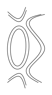
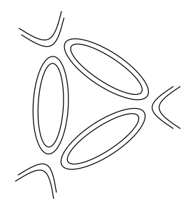
Note that the potential (4.2) is unbounded above and below, whatever the sign of $f$. An important question, raised in [5], is whether quantum corrections stabilize the potential. One can readily check that, unlike in the $D=4,\,{\cal N}=4$ SYM theory studied in [8] and used for cosmology in [6], the beta function for the coupling $f$ vanishes to leading order in the $1/N$ expansion. However, at next to leading order we find corrections from the diagrams in figures 2 and 3.

It is important to know whether ABJM theory deformed by the triple trace potential (4.2) can be defined without a UV cutoff (and if a UV cutoff is necessary, whether it influences the dynamics of interest). Since a complete analysis appears rather complicated we shall, as in Ref. [5], begin by studying simpler but analogous scalar field models sharing key features with the theory of interest. In fact, in the limit of weak ’t Hooft coupling, $N/k\to 0$, our deformation of ABJM theory precisely reduces to the $O(2N^{2})\times O(2N^{2})$ vector model at large $N$. In section 4.1, we first discuss the $O(N)$ vector model, drawing an important distinction between the cases with positive and negative coupling. In section 4.2, we then study the $O(N)\times O(N)$ vector model, which appears as the weak ’t Hooft coupling limit of the deformed ABJM model of interest. Finally, in section 4.3, we comment on the case of non-zero ’t Hooft coupling.

We would like to thank A. Bernamonti, J. de Boer, I. Klebanov and D. Tong for useful discussions, and E. Rabinovici for comments on the manuscript. In addition, we thank the anonymous PRD referee for comments leading to footnote 6 and to an improved discussion in section 4. B.C. and T.H. are grateful for the hospitality of the Centre for Theoretical Cosmology in Cambridge and Perimeter Institute for Theoretical Physics at several stages of this project. B.C. also thanks the Galileo Galilei Institute for Theoretical Physics for hospitality and INFN for partial support during the completion of this work. The work of B.C. was supported in part by the Belgian Federal Science Policy Office through the Interuniversity Attraction Pole IAP VI/11 and by FWO-Vlaanderen through project G.0428.06. The work of N.T. is supported by the Perimeter Institute for Theoretical Physics.

References

• [1] T. Hertog and G. T. Horowitz, JHEP 0407 (2004) 073 [arXiv:hep-th/0406134].
• [2] J. M. Maldacena, Adv. Theor. Math. Phys. 2, 231 (1998) [Int. J. Theor. Phys. 38, 1113 (1999)] [arXiv:hep-th/9711200].
• [3] T. Hertog and G. T. Horowitz, JHEP 0504 (2005) 005 [arXiv:hep-th/0503071].
• [4] O. Aharony, Y. Oz and Z. Yin, Phys. Lett. B 430 (1998) 87 [arXiv:hep-th/9803051].
• [5] S. Elitzur, A. Giveon, M. Porrati and E. Rabinovici, JHEP 0602 (2006) 006 [arXiv:hep-th/0511061].
• [6] B. Craps, T. Hertog and N. Turok, arXiv:0712.4180.
• [7] O. Aharony, M. Berkooz and E. Silverstein, JHEP 0108, 006 (2001) [arXiv:hep-th/0105309].
• [8] E. Witten, arXiv:hep-th/0112258.
• [9] M. Berkooz, A. Sever and A. Shomer, JHEP 0205, 034 (2002) [arXiv:hep-th/0112264].
• [10] S. R. Coleman and D. J. Gross, Phys. Rev. Lett. 31 (1973) 851.
• [11] O. Aharony, O. Bergman, D. L. Jafferis and J. Maldacena, JHEP 0810 (2008) 091 [arXiv:0806.1218 [hep-th]].
• [12] W. A. Bardeen, M. Moshe and M. Bander, Phys. Rev. Lett. 52, 1188 (1984).
• [13] E. Rabinovici, B. Saering and W. A. Bardeen, Phys. Rev. D 36 (1987) 562.
• [14] B. Craps, T. Hertog and N. Turok, in progress.
• [15] P. Breitenlohner and D. Z. Freedman, Annals Phys. 144 (1982) 249.
• [16] M. J. Duff and J. T. Liu, Nucl. Phys. B 554 (1999) 237 [arXiv:hep-th/9901149].
• [17] T. Hertog and K. Maeda, JHEP 0407 (2004) 051 [arXiv:hep-th/0404261].
• [18] M. Henneaux, C. Martinez, R. Troncoso and J. Zanelli, Annals Phys. 322 (2007) 824 [arXiv:hep-th/0603185].
• [19] M. Benna, I. Klebanov, T. Klose and M. Smedback, JHEP 0809, 072 (2008) [arXiv:0806.1519 [hep-th]].
• [20] B. E. W. Nilsson and C. N. Pope, Class. Quant. Grav. 1, 499 (1984).
• [21] M. J. Stephen and J. L. McCauley, Jr., Phys. Lett. A 44 (1973) 89; M. J. Stephen, ibid. 53 (1975) 363.
• [22] A. L. Lewis and F. W. Adams, Phys. Rev. B 18 (1978) 5099.
• [23] R. D. Pisarski, Phys. Rev. Lett. 48 (1982) 574.
• [24] S. R. Coleman and E. Weinberg, Phys. Rev. D 7 (1973) 1888.
• [25] S. S. Gubser and I. Mitra, Phys. Rev. D 67 (2003) 064018 [arXiv:hep-th/0210093].